UNIVERSIDADE DA BEIRA INTERIOR
Ciências Sociais e Humanas
The Spillover effects between USA and Euro Area:
A VECM approach with oil Prices
(Versão Definitiva após Defesa Pública)
Alexandre Almeida Lopes
Dissertação para obtenção do Grau de Mestre em
Economia
(2º ciclo de estudos)
Orientador: Prof. Doutor José Alberto Fuinhas
iv
Acknowledgements
I wish to express my sincere thanks to Professor José Alberto Fuinhas. I am extremely thankful and indebted to him for sharing expertise and encouragement to me.
I also would like to thank my family, especially my parents, for the unceasing encouragement and support through this venture. I would also wish to thank my friends and colleagues for their support and help too.
vi
Resumo
Este trabalho foca-se no efeito de spillover proveniente dos Estados Unidos da América (EUA) para a Zona Euro e o spillover da Zona Euro para os EUA, sob o efeito dos preços do petróleo. Partindo da literatura existente e aceite, são bem conhecidos os efeitos da política monetária dos EUA em outras economias, sendo em alguns casos maior e mais forte que na própria economia dos EUA. Seguindo esta linha de pensamento, este trabalho tenta, recorrendo ao Vector Error Correction Model, com dados trimestrais do primeiro trimestre de 2000 ao quarto trimestre de 2015, responder à questão de investigação: existirá efeito spillover entre estas economias e caso exista, qual a sua magnitude e direção sob o efeito dos preços do petróleo? Os resultados são consistentes com a literatura. A política monetária dos EUA é a maior fonte de propagação de choques monetários pelo mundo, especialmente para as economias desenvolvidas, como a da Zona Euro e para as economias vinculadas ao dólar. No entanto, a Zona Euro é também uma fonte de choques para a economia Americana, mas como é esperado, numa menor escala. É também demonstrado o quão importante são a oferta monetária e as taxas de juro para conter as pressões inflacionárias originadas pelos preços do petróleo, produzindo neste processo, efeitos spillover consideráveis na outra economia. Os resultados também contribuem para uma melhor compreensão, por parte dos decisores políticos, de medidas de política económica para melhor enfrentarem esta situação. Em última análise, estes resultados são facilmente entendidos, tendo em conta que ambas as economias estão integradas globalmente, sendo os EUA a economia líder. Sendo assim, não é de estranhar, que os EUA sejam a maior fonte destes choques.
Palavras-chave
vii
Resumo Alargado
Desde o início do século passado, o petróleo, a par do carvão, tem sido a principal fonte para a produção de energia no mundo, quer pelos países industrializados, quer pelos países em desenvolvimento. Pela sua multiplicidade de funções, quer como matéria-prima para a produção dos mais variados produtos como plásticos, alcatrão, borracha, vestuário entre outros, bem como a sua utilização para a produção de energia, tornam o petróleo a mais importante commodity transacionada atualmente. Tal como qualquer outra commodity, é esperada a flutuação do seu preço, gerando efeitos positivos ou negativos consoante a autossuficiência de petróleo dos países.
Por outro lado, o aumento drástico e contínuo da cotação do petróleo nos mercados internacionais poderá originar pressões inflacionárias nas economias mundiais. Desta forma, as nações vêem-se confrontadas com vários problemas. Como combater estas flutuações nas suas economias e como manter a sua economia em equilíbrio? A política monetária pode ser uma resposta para estes problemas. Através do controlo, pelos bancos centrais, das taxas de juro e/ ou da oferta monetária, as pressões inflacionárias consequentes de choques nos preços do petróleo podem ser subjugadas. No entanto, como as economias estão interligadas globalmente, as decisões de uma, terão consequências nas demais.
Esta consequência, denominada de efeito Spillover, pode ser propagada através de diversos mecanismos de transmissão da política monetária, tais como o trade channel e o financial channel. A expansão monetária de uma economia estrangeira, irá aumentar a procura estrangeira por bens domésticos, aumentando as exportações e impulsionando o output. Por outro lado, a taxa de câmbio doméstica iria apreciar, piorando a balança comercial doméstica e diminuído assim o output. Trazendo agora o foco para o financial channel, se a economia estrangeira se comporta como uma grande economia aberta, uma queda nas suas taxas de juro, poderá levar a uma queda das taxas de juro domésticas através da descida das taxas de juro globais.
Neste trabalho procurou-se responder à questão de investigação: existirá efeito spillover entre estas economias e caso exista, qual a sua magnitude e direção sob o efeito dos preços do petróleo? Para levar a bom porto a tentativa de responder a tal questão, recorreu-se a um modelo Vector Error Correction Model (VEC) para cada bloco (EUA e Zona Euro). Para tal foram utilizadas um conjunto de seis variáveis para cada modelo, sendo elas os preços do petróleo, o índice de preços do consumidor (como proxy da inflação), as taxas de juro de curto prazo, a oferta monetária, as taxas de câmbio e o PIB dos EUA e da Zona Euro. As variáveis têm um caracter trimestral e o horizonte temporal escolhido vai do primeiro trimestre de 2000 até ao
viii
quarto trimestre de 2015. Tal horizonte temporal foi escolhido devido à disponibilidade de dados referentes à Área Euro como um todo. Antes de proceder à formulação econométrica, todas as variáveis foram logaritmizadas, bem como transformadas para valores reais através do deflator do PIB.Os resultados obtidos vão de encontro à literatura analisada, relativamente à hipótese de os preços do petróleo serem uma fonte geradora de pressões inflacionárias. De referir que os preços do petróleo originam pressões inflacionárias em ambos os blocos estudados. É também constatado a grande importância das variáveis monetárias, tais como as taxas de juro, a oferta monetária, numa tentativa de os bancos centrais controlarem a inflação. Desta forma conseguimos denotar a grande influência da política monetária norte americana na criação destes choques. Podemos assim concluir que a direção do spillover é dos Estados Unidos para a Zona Euro. É também evidenciada a influência, embora em menor escala, das variáveis europeias na volatilidade do output americano, em especial a oferta monetária.
Através da análise do mecanismo de correção dos erro), é demonstrado que as entidades governamentais (Bancos Centrais) não conseguem corrigir, no curto-prazo, os desequilíbrios, o que vai de acordo com a teoria económica, quando se trabalha com variáveis monetárias. Em última análise, as conclusões podem ser feitas relativamente aos choques da política monetária americana. Os resultados obtidos seguem a literatura existente e aceite. A política monetária dos Estados Unidos continua a ser a maior fonte de choques monetários, no entanto, é também provado a importância da Zona Euro na economia americana. As conclusões obtidas são facilmente compreendidas considerando as premissas e o horizonte temporal do trabalho. Os resultados passam um conjunto de testes de diagnóstico, como a auto correlação e os testes de normalidade.
Este trabalho foi construído com base em dados de freuência trimestral dos EUA e da Zona Euro para um período de quinze anos. Para o modelo dos EUA estes dados estão facilmente disponíveis em qualquer base de dados estatal ou académica. No entanto para o caso da Zona Euro esta premissa já não é válida, pois este bloco é algo recente e a disponibilidade de dados para a mesma é escassa. Por outro lado, desde o ano 2000, ocorrem duas recessões económicas, a crise do Dotcom e a crise do Subprime, crises estas que afetaram profundamente as economias globais e a estabilidade financeira quer de instituições, quer de estados. Por conseguinte estas crises têm uma forte probabilidade de enviesarem os resultados obtidos.
Para uma abordagem futura relativamente ao tema, além de um maior espectro temporal utilizado, pode-se dividir a Zona Euro em grupos de países mais homogéneos, tornando mais fácil e clara a análise dos países mais subjetiveis a estes choques. Por outro lado, uma análise a toda a União Europeia pode ser feita, tornando os resultados mais fiáveis e robustos.
x
Abstract
This paper addresses to the spillover effects from the USA to the Euro Area and the spillover from Euro Area to the USA, under oil prices. Taking into consideration the already accepted and well-established literature is well known the effects of the USA monetary policy on other economies, being in some cases bigger and stronger than in the USA economy itself. Following this line of thought, this paper aims, supported by a VECM methodology and using quarterly data from 2000Q1 to 2015Q4, to measure the magnitude of spillover effects on both economies. The results also contribute to shed light on economic policy procedures, specially enabling the decision makers to handle this effects in their economies. The results are consistent with the literature. The USA monetary policy plays the major role on the propagation of monetary shocks across the globe, especially to the big and mature economies, such as the Euro Area and to economies linked to the USA dollar. However, the Euro Area is also a source of shocks to the USA economy but, as expected, in a smaller scale. It is also shown how important the money supply and the interest rates are to restrain the inflationary pressures originated by the oil prices, producing a sizable spillover on the other economy. Ultimately these results are easily understood, being both economies integrated in a global market dominated by the USA and consequently, is not strange, that the USA is the biggest source of these shocks.
Keywords
xii
Index
1. Introduction ... 1
2. Review of the empirical literature ... 3
2.1. Oil prices effect on economy ... 3
2.2. International transmission of monetary policy ... 4
2.3. The spillover effect ... 4
3. Empirical model ... 8
3.1 Dara description ... 8
3.2 The Vector Error Correction model ... 9
4. Empirical results ... 10
4.1. Unit roots and cointegration tests ... 10
4.2. Diagnostic tests ... 13
4.3. The long-run relationship ... 14
4.4. The short-run dynamic ... 15
4.4.1. The disequilibrium adjustment speed ... 17
6. Discussion ... 22
7. Conclusion ... 25
Appendix ... 26
xiv
Figures list
Figure 1. Inverse Roots of AR Characteristic Polynomial for Euro Area and USA Figure 2A. Response to Cholesky One S.D. Innovations – Euro Area
Figure 2B. Response to Cholesky One S.D. Innovations – USA Figure 3. VAR Granger Causality Relationships
xvi
Tables list
Table 1. Overview of the existing evidence of U.S. monetary policy spillovers Table 2A. Variable definition and summary statistics – Euro Area
Table 2B. Variable definition and summary statistics – USA Table 3A and 3B. Unit root tests – Euro Area
Table 3C and 3D. Unit root tests – USA
Table 4A. VAR Johansen’s cointegration test summary – Euro Area Table 4B. VAR Johansen’s cointegration test summary – USA Table 5A. VEC diagnostic tests – Euro Area
Table 5B. VEC diagnostic tests – USA
Table 6A. Estimated VEC model ECT’s – Euro Area Table 6B. Estimated VEC model ECT’s – USA
Table 7A. VAR Granger causality tests/ block exogeneity – Euro Area Table 7B. VAR Granger causality tests/ block exogeneity – USA Table 8A. Variance decomposition– Euro Area
Table 8B. Variance decomposition – USA
A Table 1A. Unit root tests with structural breaks Zivot-Andrews – Euro Area A Table 1B. Unit root tests with structural breaks Zivot-Andrews – USA A Table 2A. VECM long run coefficients diagnostic tests – Euro Area A Table 2B. VECM long run coefficients diagnostic tests – USA A Table 3A. VAR Lag Order Selection Criteria – Euro Area A Table 3B. VAR Lag Order Selection Criteria – USA
A Table 4A. Unrestricted Cointegration Rank Test (Trace and Maximum Eigenvalue) – Euro Area
xviii
Acronyms list
USA United States of America EUA Estados Unidos da América OILP Oil prices
CPI Consumer Price Index IRS Short-term interest rates
M2 Money supply
YEURO Euro Area GDP YUSA United States GDP
EX Exchange rate
ECT Error Correction Terms VAR Vector Auto Regression VEC Vector Error Correction
FRED Federal Reserve Economic Data
OECD Organization for Economic Co-operation and Development IRF’s Impulse Reaction Functions
1
1. Introduction
In this chapter is presented an introductory background to the theme that is proposed to be study and also the research question and the respective investigation hypothesis.
In the past century and so far, until today, oil is one of the most important stimulator of economic growth. Performing a crucial role in the industrialized world, as an important commodity which can be processed and transformed in multiple products, but more importantly has a key generator of energy. According to the USA Energy Information Administration (EIA), in 2014 USA consumed in a daily basis around 19.106 thousand barrels and Europe some 14.172 thousand, nevertheless USA where that year the biggest world producer. The World consumption has also grown from 59.522 in 1980 to something like 93.484 in 2014, so we can see how important oil is to global economy.
Oil, as a commodity, is subjected to fluctuations of its price, generating different outcomes considering the country’s oil auto-sufficiency. The countries are faced with several problems: how to counteract the effects of these fluctuations in their economies and how to maintain the economy in an even kneel? The monetary policy could be an answer to these problems. Through the central banks control of the interest rates and money supply, the inflationary pressures created by the oil price shocks could be subdue. However, most of the economies are globally linked, meaning that the decisions of ones will spillover to the others.
The spillover effect can be propagated by various monetary policy transmission channels, more particularly via the trade channel or by the financial channel. A foreign monetary expansion, by the trade channel, would increase the demand for domestic goods, raising domestic exports and boosting the output (income absorption channel). On the other way, the domestic exchange rate would appreciate, worsening the domestic trade balance and decreasing the domestic output by the expenditure switching effect (Dornbusch, 1980; Gali and Monacelli, 2005; Lubik and Schorfheide 2007; Cwik et al. 2011). By the financial channel, if the foreign country is a large open economy, a drop in the foreign interest rates can low domestic interest rates indirectly by a decrease in the world interest rates (Svensson and van Wijnbergen 1989; Gali and Monacelli 2005).
The research question that this work was built on is two folded: (i) first to prove if the oil prices are a source of monetary policy shocks and; (ii) second if these shocks propagate from one economy to others. The research hypothesis are as follows: (i) the oil prices do not generate any shock in the economies; (ii) the oil prices generate shocks in one economy, but it does not
2
propagate to the others and; (iii) the oil prices generate shocks and they propagate through the economies.In this work, a contribute is made for the understanding of the dimension and direction of the spillover between the USA and the Euro Area under oil price pressures. The spillover running from USA monetary policy shock to the Euro Area and vice-versa, is analyzed, using a Vector Error Correction Model (VECM) approach, with quarterly frequency data on a set of six time-series from 2000Q1 to 2015Q4.
The results show that oil prices are an important source of inflationary pressures to the blocks analyzed. We then notice the great importance of the monetary variables, such as short-run interest rates and money supply (M2) to counteract this inflationary pressure. Here we can see the big influence of the USA monetary policy in the Euro Area, running the spillover, from the USA to the Euro Area. However, the European variables also have a contribution to the variability of the USA output, especially the money supply and the exchange rates.
It is also shown that the entities are not able to quickly correct the disequilibrium, by analyzing the error correction terms of the model. Ultimately conclusions can be made on the USA monetary policy shocks. Our results follow the literature, being the USA monetary policy the biggest source of shocks. However, it is also demonstrated the rising importance of Euro Area conditions to the USA economy. Both conclusions are easily understood under the time span and assumptions made. These results survive a numerous battery of robustness tests, necessary to corroborate the conclusions made.
The remain of this work is organized as follow: Chapter 2. lays the empirical literature of the theme. Chapter 3. expresses the empirical model, variables and the data used; Chapter 4. expresses the main empirical results; Chapter 5. presents the robustness tests performed and their results; Chapter 6. contains the discussion; and Chapter 7. finalize the work with a brief conclusion.
3
2. Review of the empirical literature
In this chapter are stated some of the most important contributions from the main researchers in this field and their main conclusions. It is from this point then, latter, the whole work started to take shape, regarding methodology concerns, countries to study, time periods and the frequency of the data and variables to be used. In the following points is shown the major influence of oil prices in economy, how monetary policy shocks are propagated and finally is shown how the spillover effects behaves.
2.1. Oil prices effect on economy
According to the existent literature oil prices have a strong influence on the economy. Some literature (Tang et al. 2010; Miller and Ratti 2009; Huang et al. 1996 and Hamilton 1983), suggest that oil prices have a negative effect on industrial production and a positive effect on inflation. An increase in oil prices would raise production costs, generating a lower production and a lower output (Jones and Paik 2004). Jiménez-Rodriguez and Sánchez (2004) further point out the bidirectional relationship between oil prices movements and economic variables, such as inflation. Oil prices also have different effects on different countries, as also shown by Jiménez-Rodriguez and Sánchez (2004) an oil price increase would be positive for a net-oil exporter but, would be harmful for a net-oil importer. On the other side of the spectrum, Barsky and Kilian (2004), refer that an oil price shock does not cause an immediate impact on the economy.
According to Borio and White (2004) the price of assets could be seriously influenced by monetary policy decisions. Although if we consider oil prices shocks as monetary shocks, an active monetary policy is needed to fight inflationary pressures and to ensure a minimum contraction in the output (Castillo et al. 2010; Romer and Romer 1989).
There are several articles highlighting the influence of oil prices in the monetary policy decisions of central banks (e.g. Bernanke et al. 1992; Kilian 2009; Koopman et al. 2014). Focusing on the work of Castillo et al. (2010), central banks are then faced with a trade-off between inflation and output, when an oil price shock occurs, through the monetary policy response. An improved economic outcome is expected if the policy makers focus on engaging the inflationary pressures of an oil price shock, instead of focusing in stabilizing the output. The recessive consequences of an oil price shock are smaller when a central bank focus on price level (Leduc and Sill 2004).
Bernanke et al. (1997) advocate, about the recession in the USA from the period of the late 70’s to the 90’s caused by oil price shocks, that this economic downturn was mainly a result of
4
a monetary policy response from the FED, from the oil price shock itself. If the FED, had assumed a neutral policy, the output contraction would be inferior.2.2. International transmission of monetary policy
Considering a theoretical point of view, spillovers can be propagated by two different channels, via the trade and the financial channel. In the paragraphs bellow will be explained these two points of view and their related academic and scientific background through a short description of the most relevant authors and their work.
Taking focus on the trade transmission channel, an expansionary foreign monetary policy would increase the foreign demand for domestic goods, raising domestic exports and boosting domestic output (income absorption effect). On the other way, the domestic exchange rate would appreciate after this foreign expansionary monetary policy, if it is not fixed, worsening the domestic trade balance, decreasing domestic output by the expenditure switching effect (Dornbusch 1980; Gali and Monacelli 2005; Lubik and Schorfheide 2007; Cwik et al. 2011). Although, for countries with fixed exchange rates, the trade channel indicate that the domestic output will follow the same direction of foreign output by an increasing in foreign demand. In countries with flexible exchange rates, however, the fluctuations of the exchange rate counter the income absorption effect and the direction of the spillover is a priori ambiguous. In this case, which effect will prevail depends on the domestic countries openness degree and the elasticity of substitution between domestic and foreign goods (Gali and Monacelli 2005). Monetary policy shocks can also be propagated internationally via the financial channel, if we are in presence of a strong financial integration between countries, independently of the level of trade integration and exchange rate regime. Pointing out the foreign country as a large open economy, a drop in a foreign interest rate can low domestic interest rates, indirectly by a decline in the world interest rates (Svensson and van Wijnbergen 1989; Gali and Monacelli 2005).
2.3. The spillover effect
It is being argued that the global economic conditions and growth are influenced by a global financial cycle, which seems to be determined by the USA monetary policy (Bekaert et al. 2013; Rey and Helene 2013).
Evidences suggest that spillovers resultants of the monetary policy could be important sources of macroeconomic and financial instability. This arise crucial questions if the central banks should have in to consideration the non-intentional consequences of their actions on the others and how to promote stability (Chen et al. 2016).
5
Taking into consideration recent studies about the asset purchases of the USA, (Neely 2010), found that the quantitative easing of the USA, caused a drop in the bond rates, in 20 to 80 basis points, in other advanced economies. Glick and Leduc (2011), had shown that the commodities prices had fall, when the USA asset purchase was announced.On other work, by Kim (2001), the transmission of USA monetary shocks to non-USA, G-6 countries was studied, being proved the existence of a positive spillover running from the USA to the other non-USA, G-6 countries, following a USA monetary expansion. This positive spillover appears to happen through the world capital market. An USA monetary expansion in the short-run produces a fall in the balance trade but, improving in a medium and long-short-run. Second, the monetary expansion of the USA creates a boom in the non-USA G-6 countries, being the changes in the trade balances too small to explain the booms, while the increase in the world aggregate demand (through the world real interest rate changes), appears to have a major role in the transmission.
Canova (2005), in his work on the transmission of shocks from the USA to the Latin American countries, found that USA monetary shocks produce significant responses in crucial economic variables, especially the interest rates playing a major role in that transmission. Second, a USA monetary contraction produce a strong and fast increase in the Latin American interest rates, which is translated in a price increase and a depreciation in the real exchange rate. Ultimately, the USA disturbances are an important source of variability on Latin American economic variables.
Maćkowiak (2007), reached the same conclusions than Canova, for developing economies, also adding that the price level and real output response to these shocks are greater in these economies than in the price level and real output of USA itself. In conclusion, an USA monetary policy shock affects the interest rates and the exchange rate in an emerging market quickly and strongly. Following an USA monetary contraction, the currency in these markets tend to depreciate, leading to a growth in inflation. A depreciation in the exchange rate leads to an increase in the exports, but an increase in the interest rates tends to decrease consumption and investments.
Jannsen and Klein (2011) also found that an Euro Area monetary policy shock produce a significant effect on interest rates and output in five non-Euro countries. Hájek and Horváth (2016) on their analysis on the transmission of Euro Area interest rate shocks to a set of non-Euro countries found similar output responses, with small economies reacting more effusively than the Euro Area itself.
Aizenman et al. (2016) found that financial spillovers from USA monetary policy and other core countries are larger in economies with less flexible exchange rates and with higher financial openness.
6
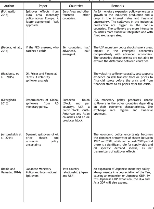
In another work concerning the effects of Euro Area contractionary monetary policy in Poland, Czech Republic and Hungary, Benkovskis et al. (2011) found that these countries exchange rates depreciate, prices raised, and real activity variables decline due to reduced foreign demand. The literature about this theme is very extensive and to keep this work easier to be scrutinized, will only be referred some of the most important authors and their recent works, which will be referenced in the table 1, shown below.Table 1. Overview of the existing evidence of USA monetary policy spillovers
Author Paper Countries Remarks
(Potjagailo
2017) Spillover effects from Euro area monetary policy across Europe: A factor-augmented VAR approach.
Euro Area and other fourteen other countries.
An EA monetary expansion policy generates a growth in the industrial production and a drop in the interest rates and financial uncertainty. The spillovers in the industrial production are bigger in the non-EA countries. The spillovers are more intense in countries more financial integrated and with fixed exchange rates.
(Dedola, et al.,
2016) If the FED sneezes, who catches a cold? 36 countries, half advanced, half emergent.
The USA monetary policy shocks have a great impact in the emergent economies comparatively with advanced economies. The countries characteristics are not able to explain the difference between countries.
(Nazlioglu, et
al., 2015) Oil Prices and Financial Stress: A volatility spillover analysis
The volatility spillover causality test supports evidence on risk transfer from oil prices to financial stress before the crisis and from financial stress to oil prices after the crisis.
(Georgiadis
2015) Determinants of Global spillovers from US monetary policy.
European Union (Block and per country), USA, a Baltic clock, south-American and Asian countries and an oil producer block.
USA monetary policy generates sizable spillovers in the other countries depending on their economic characteristics, like exchange rate regime and financial openness.
(Antonakakis et
al. 2014) Dynamic spillovers of oil price shocks and economic policy uncertainty
The economic policy uncertainty becomes the dominant transmitter of shocks between 1997 and 2009, while in the post-2009 period there is a significant role for supply-side and oil specific demand shocks, as net transmitters of spillover effects.
(Dekle and
Hamada, 2014) Japanese Monetary Policy and International Spillovers.
Two country relationship (Japan and USA)
An expansion of Japanese monetary policy always results in a depreciation of the Yen, causing an expansion on Japanese GDP. By this Japanese GDP expansion, the USA and Asia GDP will also expand.
7
(Ilzetzki and
Jin, 2013) The Puzzling Change in the international Transmission of U.S. Macroeconomic Policy Shocks.
USA and the other eight biggest economies.
A one percentage point raise in the FFR produce a sizable drop in foreign production. The drop magnitude is similar, but slightly smaller, than the output drop found in the USA.
(Abiad et al.
2013) Dancing Spillovers, Together? Common Shocks, and the Role of Financial and Trade Linkages. World Economic Outlook, October 2013.
Asia, Europe and
Latin America. The USA monetary policy shocks spillovers through interest rates, being the economies pledged to the US dollar more affected. The spillovers originated by the USA still are the most important worldwide, however, the EA, China and Japan are important sources of spillovers in their regions.
(Fukuda 2013) Cross-country
Transmission Effect of the U.S. Monetary Shock
under Global
Integration.
G7 and Australia, other advanced European economies and emergent Latin American and Asian economies.
Separately analyzing the 90´s and 2000’s decades has been proved the weakening of the spillover effect from the USA. An USA contractionary policy generated adverse effects in the other countries production during the 90´s. In the next decade that effect faded way.
(Bluedorn and
Bowdler, 2011) The consequences of U.S. open economy monetary policy.
USA, Germany, UK, Canada, France, Italy and Japan.
After an USA monetary policy shock, resulted by a monetary contraction, the exchange rate appreciates. There’s also a positive spillover of the USA interest rates to the other countries. The output reacts negatively, indicating the effects of the USA monetary contraction. The USA suffer the same effect, mas in a minor scale.
(Neri and
Nobili, 2006) The monetary policy shocks transmission of from the US to the euro area.
USA and Euro Area. An USA monetary contraction have a positive effect in the EA output in the short-run, ceasing in the medium-run. A sudden rise in the FFR produce a depreciation of the euro against the dollar. The trade balance mechanism is insignificant.
To conclude, we can state that the USA monetary policy is the main driving force of the creation and propagation of these shocks throughout the global open economies. On the other hand, is also demonstrated that usually the direction of the spillovers goes from the leader economy to the followers.
Focusing on the conclusions of the work of the previous authors, is stated the major importance of the interest-rates in the propagation of monetary shocks. However, the countries characteristics, like trade and financial openness and exchange rate regime are also some important variables to the propagation of these shocks. Some of these works also state the weakening of the USA influence in the global financial cycle, with the developing of the new global economies, like China and India, nonetheless the USA are still the major generator of monetary policy shocks. On another point is refereed that in some countries the effects of the USA monetary policy shocks are more intense than in the USA itself.
8
3. Empirical model
The empirical analysis is based on a Vector Error Correction Model for two blocks, the European and the north American one, using a set of six time-series for both models. In the following subsection, will be explained this approach and the data used to mount it.
3.1 Data description
The model was mounted using a set of six time-series for each model. The data was extracted from FRED, Eurostat and OECD. The data cover the period from 2000Q1 to 2015Q4 and include the oil prices from Oklahoma for the American model and London for the European model, Consumer price index (CPI), short-term interest rates, money supply (M2), the exchange rates and the GDP for Euro Area and USA. The time span used was chosen concerning the availability of data for the Euro Area as an all.
The rationale behind the choose of these variables is easily understood according what this work attempts to accomplish. The oil prices were used to perform as a shock to measure the reaction of the monetary policy variables as interest rates and money supply. The CPI was used to test if the oil prices indeed caused inflation and how the interest rates and money supply behave towards it. Money supply, interest rates and exchange rates work here as a proxy of the central banks response to the inflationary pressures created by the oil prices. Lastly both GDP from USA and Euro Area serve to measure the effects of central bank’s monetary policy spillover on one on other.
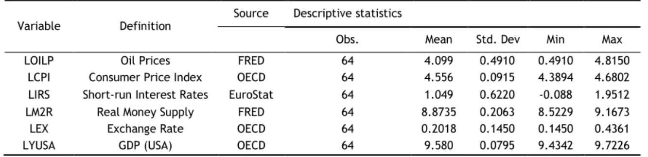
Table 2A. Variable definition and summary statistics – Euro Area
Variable Definition Source Descriptive statistics
Obs. Mean Std. Dev Min Max
LOILP Oil Prices FRED 64 4.099 0.4910 0.4910 4.8150
LCPI Consumer Price Index OECD 64 4.556 0.0915 4.3894 4.6802 LIRS Short-run Interest Rates EuroStat 64 1.049 0.6220 -0.088 1.9512
LM2R Real Money Supply FRED 64 8.8735 0.2063 8.5229 9.1673
LEX Exchange Rate OECD 64 0.2018 0.1450 0.1450 0.4361
LYUSA GDP (USA) OECD 64 9.580 0.0795 9.4342 9.7226
Table 2B. Variable definition and summary statistics – USA
Variable Definition Source Descriptive statistics
Obs. Mean Std. Dev Min Max
LOILP Oil Prices FRED 64 4.0935 0.4235 3.2042 4.8407
LCPI Consumer Price Index OECD 64 4.5486 0.1065 4.3554 4.6940 LIRS Short-run Interest Rates OECD 64 0.0444 1.4511 -2.2487 2.0998
LM2R Real Money Supply FRED 64 8.9668 0.1863 8.6685 9.3254
LYUSA GDP (USA) OECD 64 9.5880 0.0795 9.4342 9.7226
9
The data were transformed before the analysis. Natural logarithms were performed for all the variables. The oil prices, money supply, GDP, interest rates and exchange rates were transformed to real values using the GDP deflator. In tables 1A. and 1B., are shown the description of the variables and their summary statistics.3.2 The Vector Error Correction model
The VEC model is a multiple time-series model commonly used for data with a long-run stochastic trend, also known as cointegration. This model is useful to estimate both the short-run and long-short-run effects of one time-series to the other. The cointegration VAR approach has the advantage of allowing a different set of variables to adjust and respond to disturbances observed in the other, so that the system converges to the long-run equilibrium (Marques et al. 2014).
Johansen and Juselius (1990), and Johansen et al. (1999) assume that there may be n – 1 cointegrating vectors. Long-run relationships between the variables will be tested. The Johansen method was used with a conditional VEC model with k lags as shown in equation (1):
t t k t i t k i i t
X
X
CD
X
1 (1) where 𝑋𝑡 is the vector of endogenous variables; 𝐷𝑡 is the vector of exogenous variables;
𝑖and C are the coefficient matrices of endogenous and exogenous variables, respectively. The matrices
𝑖 control the short-run dynamics of the model, while the long-run cointegration relationships are captured by the matrix
.
The term
tdenotes the residuals, which are
serially and mutually independent. The solution proposed by Johansen (1995) depends on the testing of the rank 𝒓 ≪ 𝟓 of the matrix
. No cointegration relationships exist when 𝑟 = 0.
Otherwise, a small rank 𝑟 means that there are 𝑟 possible stationary linear combinations. The decision between the use of a VAR or VEC model is a question of the existence of only short-run or both, short and long-short-run effects (Marques et al. 2014).10
4. Empirical results
This section includes the empirical results. In the following sections are presented the unit roots and the cointegration tests for both models, as the long-run cointegration relationships and the short-run dynamics.
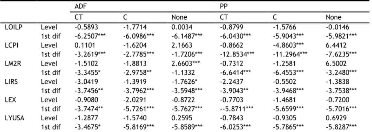
4.1. Unit roots and cointegration tests
In this subsection, the stationary properties of the variables used in the analysis is examined for both models. A visual inspection of the variables behavior stat that all of them are non-stationary.
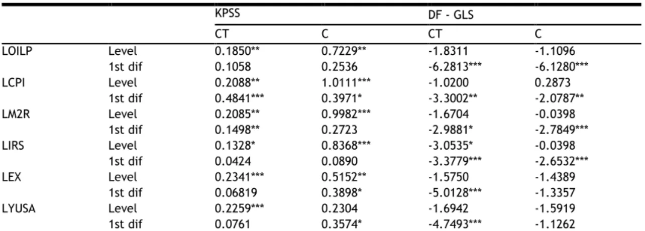
The stationary of the series was then tested with different unit root tests: (i) the Augmented Dickey – Fuller test; (ii) the Phillips Perron (PP) test; (iii) the Kwiatkowski Phillips Schmidt Shin (KPSS) test and (iv) the Dickey – Fuller GLS (DF – GLS) test. The ADF have the null hypothesis of a unit root. The Schwarz criterion of 10 lags was used for both models. The PP test also have the null of a unit root and the Newey-West Bandwidth was used. The KPSS test has the null hypothesis of stationarity and was executed with the Bartlett kernel spectral estimation and Newey-West Bandwidth. The Dickey-Fuller GLS test has the null of a unit root and the Schwarz criterion was used concerning the lag selection. The results are displayed in the tables 3A to 3D. The main concern of using all four tests is to achieve a robust result of the series stationarity. Tables 3A to 3D show the results of the tests, both in levels and in first differences.
Table 3A. ADF and PP Unit root tests – Euro Area
ADF PP CT C None CT C None LOILP Level -0.5893 -1.7714 0.0034 -0.8799 -1.5766 -0.0146 1st dif -6.2507*** -6.0986*** -6.1487*** -6.0430*** -5.9043*** -5.9821*** LCPI Level 0.1101 -1.6204 2.1663 -0.8662 -4.8603*** 6.4412 1st dif -3.2619*** -2.7785*** -1.7206*** -12.8534*** -11.2964*** -7.6235*** LM2R Level -1.5102 -1.8813 2.6603*** -0.7312 -1.2581 6.5002 1st dif -3.3455* -2.9758** -1.1332 -6.6414*** -6.4553*** -3.2480*** LIRS Level -3.0419 -1.3919 -1.7626* -2.2437 -0.5502 -1.3838 1st dif -3.7456** -3.7962*** -3.5948*** -3.9043** -3.9468*** -3.7538*** LEX Level -0.9080 -2.0291 -0.8722 -0.7703 -1.4681 -0.7200 1st dif -3.7474** -5.7261*** -5.7627*** --5.8711*** -5.6599*** -5.7016*** LYUSA Level -1.2877 -1.5740 0.2595 -0.7843 -0.9305 0.6929 1st dif -3.4675* -5.8169*** -5.8589*** -6.0253*** -5.7865*** -5.8287*** Notes: ADF stands for Augmented Dickey Fuller test; PP stands for Philips Perron test;; CT stands for constant and trend; C stands for constant; ***, ** and * represent statistically significant level for 1%, 5% and 10%, respectively.
11
Table 3B. KPSS and DF-GLS Unit root tests – Euro Area
KPSS DF - GLS CT C CT C LOILP Level 0.1850** 0.7229** -1.8311 -1.1096 1st dif 0.1058 0.2536 -6.2813*** -6.1280*** LCPI Level 0.2088** 1.0111*** -1.0200 0.2873 1st dif 0.4841*** 0.3971* -3.3002** -2.0787** LM2R Level 0.2085** 0.9982*** -1.6704 -0.0398 1st dif 0.1498** 0.2723 -2.9881* -2.7849*** LIRS Level 0.1328* 0.8368*** -3.0535* -0.0398 1st dif 0.0424 0.0890 -3.3779*** -2.6532*** LEX Level 0.2341*** 0.5152** -1.5750 -1.4389 1st dif 0.06819 0.3898* -5.0128*** -1.3357 LYUSA Level 0.2259*** 0.2304 -1.6942 -1.5919 1st dif 0.0761 0.3574* -4.7493*** -1.1262
Notes: KPSS stands for Kwiatkowski-Philips-Schmidt-Shin test; DF – GLS stands for Dickey Fuller GLS; CT stands for constant and trend; C stands for constant; ***, ** and * represent statistically significant level for 1%, 5% and 10%, respectively
The results support that all the variables have a unit root, i.e. being I-(1). The tests corroborate the visual inspection of the variables.
Table 3C. ADF and PP Unit root tests – USA
ADF PP CT C None CT C None LOILP Level -0.8849 -1.9557 -0.1091 -1.0828 -1.7086 -0.1102 1st dif -6.3270*** -6.2391*** -6.2913*** -6.2512*** -6.0589*** -6.1257*** LCPI Level -0.1195 -2.0912 5.7368 -1.1121 -2.9178** 6.0387 1st dif -9.2155*** -8.7275*** -2.5165** -9.1225*** -6.4391*** -5.5145*** LM2R Level -1.7252 0.1720 4.0949 -1.4389 0.2549 8.2902 1st dif -5.0658*** -5.085*** -2.6935*** -5.0658*** -5.085*** -2.6935*** LIRS Level -1.8273 -1.6128 1.6461 -1.6913 -1.3226 -1.3920 1st dif -4.7201*** -4.7116*** -4.6502*** -4.7038*** -4.6992*** -4.6311*** LYUSA Level -1.6005 -0.4112 2.9626 -1.8068 -0.9567 4.0849 1st dif -5.4728*** -5.5379*** -4.4162*** -5.5464*** -5.6081*** -4.4604*** LYEURO Level -0.8749 -2.1164 0.5834 -0.7608 -1.5750 0.6415 1st dif -4.1082** -5.4983*** -5.4924*** -5.6051*** -5.3574*** -5.4329*** Notes: ADF stands for Augmented Dickey Fuller test; PP stands for Philips Perron test;; CT stands for constant and trend; C stands for constant; ***, ** and * represent statistically significant level for 1%, 5% and 10%, respectively.
Table 3D. KPSS and DF-GLS Unit root tests – USA
KPSS DF - GLS CT C CT C LOILP Level 0.2077** 0.6542** -2.0425 -1.2699 1st dif 0.1129 0.2459 -6.4130*** -6.2766*** LCPI Level 0.2116** 1.008*** -0.5525 0.8260 1st dif 0.2490*** 0.3719* -8.7569*** -3.4774*** LM2R Level 0.1754** 1.013*** -1.8095 1.4926 1st dif 0.0937 0.1280 -5.1355*** -5.1207*** LIRS Level 0.1217* 0.7853*** -1.9596 -0.8913 1st dif 0.0989 0.1018 -4.6853*** -4.4197*** LYUSA Level 0.1445* 0.9526*** -1.5864 1.4231 1st dif 0.1001 0.1308 -4.3397*** -3.0414*** LYEURO Level 0.2419*** 0.6216** -1.5060 -1.1763 1st dif 0.0622 0.4499* -4.9875*** -1.2791
Notes: KPSS stands for Kwiatkowski-Philips-Schmidt-Shin test; DF – GLS stands for Dickey Fuller GLS; CT stands for constant and trend; C stands for constant; ***, ** and * represent statistically significant level for 1%, 5% and 10%, respectively
12
Concerning the lag selection, two criteria were used to select the optimal number of lags in the VAR estimation: the Schwarz and the Hannan-Quinn criteria. The Schwarz criterion is more restrictive in the lag selection than the Hannan-Quinn. Both were used in the models, suggesting 4 lags for the European model and 5 lags for the American one. This information is presented in the tables A 2A and A 2B in the appendices section.In the VEC model equation, the vector of endogenous variables, 𝑋𝑡= [DLOILP, DLCPI DLM2, DLEX,
DLYUSA], and the vector of the exogenous variables is 𝐷𝑡= [DLIRS, ID1, SD2] for the European
model. For the U.S. model, 𝑋𝑡= [DLOILP, DLCPI DLM2, DLIRS, DLYEURO], and the vector of the
exogenous variables, 𝐷𝑡= [DLYUSA, SD3, SD4]. The exogenous variables are consistent with the
results from the exogeneity tests. The dummies (ID1, SD2, SD3 and SD4) were chosen taking into consideration the Zivot-Andrews test for structural breaks and it was performed both for levels and first differences, which are present in the appendix section. The control dummy ID1 is an impulse dummy for the 2013Q3 period and the control dummy SD2 is a seasonal dummy for the time span of 2006Q4 to 2007Q4. For the American model, the dummy SD3 and SD4 are seasonal dummies for the time period of 2007Q1 to 2007Q4 and 2008Q3 to 2009Q1 respectively.
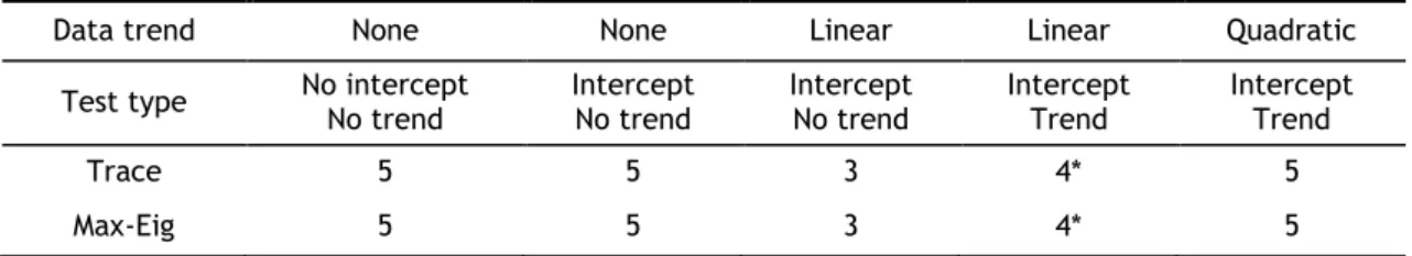
The results of the VAR Johansen´s cointegration test are shown in the tables 4A and 4B. The tables show both the results for the Trace and Max-Eig criteria, the trend and the test type. Both tables denote the existence of cointegrated vectors within the models. The order of the variables is the same as the table 1. The rationale behind the ordering of the variables was the Cholesky variables ordering, which means the variables are ordered in a decreasing order of exogeneity, i.e. oil prices are more likely to influence inflation than the other way around. The VAR treats the variables LIRS and LYUSA as exogenous for the European and American model respectively.
Table 4B. VAR Johansen’s cointegration test summary – USA
Data trend None None Linear Linear Quadratic
Test type No intercept No trend Intercept No trend Intercept No trend Intercept Trend Intercept Trend
Trace 5 5 3 4* 5
Max-Eig 5 5 3 4* 5
Table 4A. VAR Johansen’s cointegration test summary – Euro Area
Data trend None None Linear Linear Quadratic
Test type No intercept No trend Intercept No trend Intercept No trend Intercept Trend Intercept Trend
Trace 3 3 3 4 4*
13
Following the VAR Johansen tests, the VEC was executed with four cointegrated vectors for both models. Nevertheless, the European one was constructed with a quadratic trend and intercept and the American model was mounted with a linear trend and intercept. Both the Trace and Max-Eigenvalue Statistic tables are presented in the appendices section for both models.4.2. Diagnostic tests
This section concerns about the diagnostic tests of the model estimation. A battery of tests was performed and can be examined in next tables. Several problems were checked in this section: (i) the autocorrelation and (ii) the normality of the residuals. The heteroskedasticity was not checked because of the few degrees of freedom present in the model, a consequence of the reduced number of observations used.
Table 5A. VEC diagnostic tests – Euro Area
Normality tests Autocorrelation LM test
Component Skewness Chi-sq Kurtosis Chi-Sq Jarque - Bera Lags LM - Stat LOILP -0.3768 1.3966 3.2924 0.2103 1.6069 1 29.1503 LCPI -0.0795 0.0622 2.1622 1.7253 1.7876 2 35.7850 LM2R -0.0821 0.0663 3.3882 0.3705 0.4369 3 18.4348 LEX 0.2091 0.4299 3.0837 0.0172 0.4472 4 26.9061 LYUSA 0.0547 0.0294 3.1154 0.0327 0.0622 5 22.3217 Joint 1.9847 2.3562
Concerning the normality tests, for Euro Area, the Jarque-Bera test, demonstrate the normality of the residuals for all series. The autocorrelation study of the model by the Lagrange Multiplier test shows the absence of autocorrelation in the model, with the only exception of the lag 2.
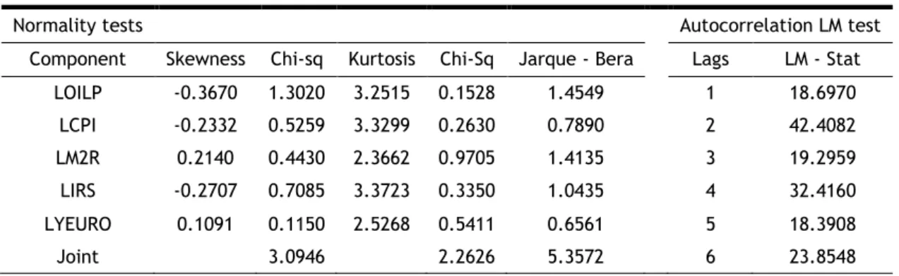
Table 5B. VEC diagnostic tests – USA
Normality tests Autocorrelation LM test
Component Skewness Chi-sq Kurtosis Chi-Sq Jarque - Bera Lags LM - Stat LOILP -0.3670 1.3020 3.2515 0.1528 1.4549 1 18.6970 LCPI -0.2332 0.5259 3.3299 0.2630 0.7890 2 42.4082 LM2R 0.2140 0.4430 2.3662 0.9705 1.4135 3 19.2959 LIRS -0.2707 0.7085 3.3723 0.3350 1.0435 4 32.4160 LYEURO 0.1091 0.1150 2.5268 0.5411 0.6561 5 18.3908 Joint 3.0946 2.2626 5.3572 6 23.8548
14
For the USA model, the Jarque-Bera test of normality reveals strong evidence of normality for all series of the model. The Lagrange Multiplier test shows the exclusion of autocorrelation, with the only exception in lag 2. To demonstrate the model robustness is shown in the figure bellow the graphics of the Inverse Roots of AR Characteristic Polynomial for both models.-1.5 -1.0 -0.5 0.0 0.5 1.0 1.5 -1.5 -1.0 -0.5 0.0 0.5 1.0 1.5 Inverse Roots of AR Characteristic Polynomial
Fig1. Inverse Roots of AR Characteristic Polynomial for Euro Area and USA respectively
4.3. The long-run relationship
Accordingly, the Johansen´s technique, the long run cointegration relationships are as follow:
LOILP = -11.9294 + 0.9096LYUSA - 0.0217t Eq. (2)
(1.2797) [0.4772]
LCPI = -4.5263 + 0.0134LYUSA - 0.0048t Eq. (3)
(0.0409) [0.7421]
LM2R = -12.5054 + 0.4246LYUSA - 0.0107t Eq. (4)
(0.0658) [0.0000]
LEX = -10.8337 + 1.1465LYUSA - 0.0039t Eq. (5)
(0.0196) [0.0000]
Focusing only in the statistically significant variables, being the std. errors in parentheses and p-value in brackets, of the equations above, we can see that a raise of 1% in the North American GDP, has a positive consequence in both money supply and exchange rate. The results of equation (4) can be explained as a precautionary measure to prevent inflation caused by the USA. The equation (5) show us that a raise in the USA GDP of 1%, produce a raise in the exchange rate, what is understandable.
LOILP = 38.6539 - 4.0919LYEURO - 0.1288t Eq. (6)
(1.4060) (0.0472) [0.0050] [0.4673]
LCPI = -3.6258 - 0.0816LYEURO - 0.0049t Eq. (7)
(0.0133) (0.0004) [0.0000] [0.0000]
15
LM2R = -9.3527 + 0.1142LYEURO - 0.0210t Eq. (8)
(0.0864) (0.0028) [0.1860] [0.0000]
LIRS = -57.5272 + 4.5378LYEURO + 0.4377t Eq. (9)
(2.4563) (0.0794) [0.0646] [0.0000]
The long run relationships in the American model could be explained easily. In equation (6), a raise of 1% in the Euro Area GDP, produce a 4% drop in the oil price in the USA, what is not yet well understood. Equation (7) shows that a raise in the Euro GDP, generates a very small fall in the USA inflation (0.081%), which is statistically insignificant.
4.4. The short-run dynamic
In this section is intended to shed some light to the models short-run dynamics. Accordingly, to the economy rationale when we work with real economy variables like interest rates, inflation and money supply it is not expected to encounter a very strong short-run reaction, because a change in one variable only produce a reaction in another after a long period of time.
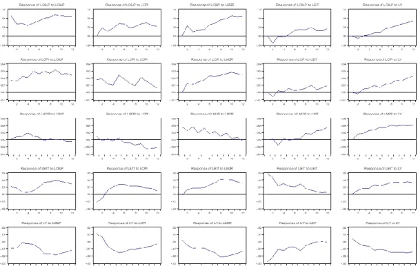
In order to understand the behavior of each variable confronted with an increase in a single variable, as well as the duration of its effect, the impulse response functions (IRF’s) are shown. The figure illustrates that one standard deviation shock on LOILP, generates a positive and powerful response to LCPI. The response of LM2R to a one standard deviation of LCPI is negative in the long-run, illustrating an attempt to subdue inflation by the central banks. Finally, the response of LY to a one standard deviation of LCPI is negative in the short-run but tends to become null in the long-run, proving the negative effect of inflation in the GDP growth. Concerning the USA response, is shown that one standard deviation of LOILP generates a positive and strong response of LCPI, as expected. On the other hand, the response of LOILP to one standard deviation of LY is positive and permanent, which demonstrates the dependence of economy on oil. The reaction of LM2R to one standard deviation of LCPI is positive in the short-run but becomes negative in the long-run, demonstrating that the Central Banks tries to subdue inflation by the raise of money supply. Analyzing the response of LM2R to a shock of LY, is shown the negative and persistent effect of the second on the first. This goes in line with the economic theory. To conclude same of the responses have not expected behaviors. There are some reasons for this situation, as the short period of time analyzed, and the nature of the variables used.
Briefly concluding this section, the responses behavior and intensity are as expected, not just by the economic theory but also by what this work aims to conclude: a positive reaction of CPI to an oil price raise, a negative response of money supply to this inflation raise in order to subdue it and the positive effect that the GDP growth has in the oil prices, proving how dependent these economies are on fossil fuels in their economic system.
16
Fig. 2A. Response to Cholesky one S.D. Innovations – Euro Area
Fig. 2B. Response to Cholesky one S.D. Innovations – Euro Area
Figure 2A. Response to Cholesky One S.D. Innovations – Euro Area
17
4.4.1. The disequilibrium adjustment speed
In the VEC model, which comprehends cointegration, is required that at least one of the coefficients of the error correction terms to be statistically significant. This condition is observed in both models. For the Euro Area, DLOILP and DLCPI, have a statistically high value for ECT1 and ECT2 respectively, indicating that the disequilibrium of oil prices is approximately 91% corrected within one quarter and CPI is corrected about 10% within one quarter.
Table 6A. Estimated VEC model ECT’s – Euro Area
DLOILP DLCPI DLM2R DLEX DLYUSA
ECT1 (-4.9296) -0.9068 (0.1672) -0.0007 (0.5043) 0.0038 (-2.7422) -0.1944 (2.855) 0.1956 ECT2 (5.4245) 25.7658 (-0.8255) -0.1018 (-1.7288) -0.3388 (3.6683) 6.7173 (-3.8929) -6.8867 ECT3 (-0.0566) -0.0458 (0.9851) 0.0207 (-0.7071) -0.0236 (2.6834) 0.8387 (-3.0569) -0.9231 ECT4 (-1.9354) -4.2902 (-3.3770) -0.1944 (4.2069) 0.3847 (0.0895) 0.0765 (-0.1059) -0.0874 R-squared 0.8678 0.9376 0.8937 0.6934 0.7064 Adj. R-squared 0.7160 0.8659 0.7717 0.3415 0.3694 F-statistic 5.7191 13.087 7.3269 1.9706 2.0962
Note: t-statistics in parenthesis
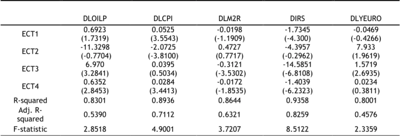
Concerning the American model, at least one of the error correction terms is also significant. DLOILP and DLCPI, do not have a short-run dynamic in this model, not being statistically relevant. Both variables have a long-run relationship in this case. However, DLM2 is statistically significant in the ECT3, being around 31% of the disequilibrium corrected within one quarter. DLIRS have a value superior to 1, so I do not considerate it to the short-run dynamic of the model.
Table 6B. Estimated VEC model ECT’s – USA
DLOILP DLCPI DLM2R DIRS DLYEURO
ECT1 (1.7319) 0.6923 (3.5543) 0.0525 (-1.1909) -0.0198 (-4.300) -1.7345 (-0.4266) -0.0469 ECT2 (-0.7704) -11.3298 (-3.8100) -2.0725 (0.7717) 0.4727 (-0.2962) -4.3957 (1.9619) 7.933 ECT3 (3.2841) 6.970 (0.5034) 0.0395 (-3.5302) -0.3121 (-6.8108) -14.5851 (2.6935) 1.5719 ECT4 (2.8453) 0.6352 (3.4413) 0.0284 (-1.8535) -0.0172 (-6.2323) -1.4039 (0.3811) 0.0234 R-squared 0.8301 0.8936 0.8644 0.9358 0.8001 Adj. R-squared 0.5390 0.7112 0.6321 0.8259 0.4576 F-statistic 2.8518 4.9001 3.7207 8.5122 2.3359
18
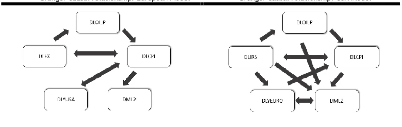
The causal relationships between variables were performed using the Granger causality/block exogeneity test for both models. When a variable helps to predict the behavior of another variable then a causal relationship is present. The Granger causality relationships detected, for the European model, are as follow: DLOILP→DLCPI; DLCPI→DLM2; DLCPI→DLEX;DLCPI↔DLYUSA; DLEX→DLOILP; DLEX→DLCPI. For the USA, the causal relationships are: DLOILP→DLCPI; DLOILP→DLM2; DLCPI↔DLIRS; DLM2↔DLYEURO; DLIRS→DLOILP; DLIRS→DLM2; DLIRS→DLYEURO; DLYEURO→DLCPI.
Table 7B. VEC Granger causality tests/ block exogeneity – USA
Dependent variables
DLOILP DLCPI DLM2 DLIRS DLY
DLOILP does not cause - 25.2916*** 14.8009** 5.6370 4.0956
DLCPI does not cause 10.8522 - 9.1235 16.8820*** 5.1725
DLM2 does not cause 2.1187 5.5210 - 8.4116 42.5942**
DLIRS does not cause 20.4434*** 29.5963*** 16.9797*** - 24.8455*** DLY does not cause 4.5387 15.9402*** 15.6782*** 1.2099 -
All 39.8303 55.2053 46.2886 111.0295 32.0180
Notes: “All” means the Granger causality test set for all independent variables. Wald tests based on 𝑥2 statistic,
with 5 df, except for “All”, 20 df.
Table 7A. VEC Granger causality tests/ block exogeneity – Euro Area
Dependent variables
DLOILP DLCPI DLM2 DLEX DLY
DLOILP does not cause - 11.6762** 8.8113* 1.0866 1.7026
DLCPI does not cause 1.4893 - 11.9871** 11.6104** 12.4035**
DLM2R does not cause 9.2760 3.6593 - 3.9821 2.9909
DLEIT does not cause 9.7877* 16.8637*** 1.4380 - 0.3990
DLY does not cause 11.5211** 18.6729*** 1.6974 0.4873 -
All 60.3922 48.4138 29.6508 31.5629 33.4752
Notes: “All” means the Granger causality test set for all independent variables. Wald tests based on 𝑥2 statistic, with
19
As seen in the figures bellow the USA model have much more causal relationships among variables than the European one. This prove the endogeneity of the variables and confirms the use of the VEC methodology.Granger causal relationship: European Model Granger causal relationship: USA Model
Figure 3. VEC Granger Causality Relationships
The exogeneity block confirms the choice of analysing the variables LIRS and LYUSA as exogenous, reinforcing the use of the VEC model approach. On the other end, the variance decomposition tries to capture the intensity of the response of one variable to the shocks of the other variables. The next tables show the results of the variance decomposition for first, fourth, eighth and twelfth quarters.
20
Table 8A. Variance decomposition of LOILP, LCPI, LM2R, LEX and LYUSA – Euro Area
Quarter S.E. LOILP LCPI LM2 LEX LYUSA
Decomposition of LOILP 1 0.0867 100.0000 0.0000 0.0000 0.0000 0.0000 4 0.1270 70.8083 12.4515 8.1468 7.6730 0.9202 8 0.1877 52.6923 22.1309 13.2798 11.1979 0.6988 12 0.2561 38.6304 26.7280 20.9415 13.0730 0.6233 Decomposition of LCPI 1 0.0022 42.5286 57.4713 0.0000 0.0000 0.0000 4 0.0041 43.7539 42.2136 10.2971 2.4548 1.2803 8 0.0063 43.0093 36.2377 16.4053 2.9722 1.3752 12 0.0078 34.8949 35.7884 21.5205 6.8148 0.9813 Decomposition of LM2R 1 0.0035 0.1456 2.4254 97.4288 0.0000 0.0000 4 0.0066 4.6309 1.8824 65.7433 6.4444 21.2988 8 0.0099 2.5766 3.3597 42.2819 6.9238 44.8578 12 0.0152 1.1030 6.1373 21.7178 18.9923 52.0493 Decomposition of LEX 1 0.0334 11.0359 8.2852 0.1672 80.5116 0.0000 4 0.0550 8.4742 7.4564 10.4598 69.2517 4.3576 8 0.0829 9.2883 10.1440 18.2192 43.1885 19.1598 12 0.0966 10.1547 7.8236 21.2441 34.5625 26.2149 Decomposition of LYUSA 1 0.0322 9.1707 9.2420 0.0106 80.0637 1.5129 4 0.0519 7.8052 9.4360 10.9053 69.0931 2.7602 8 0.0760 9.2659 13.1130 19.3068 41.6668 16.6473 12 0.0864 10.4810 10.4783 22.9055 33.4611 22.6739
Notes: Cholesky´s Ordering: LOILP, LCPI LM2, LEX, LYUSA
The Variance decomposition of the time series in a VEC model shows how much of the future variability of one time series is due to shocks into the others time series of the system. The results demonstrate that LOILP explain about 42% of the forecast error variance of LCPI in the first quarter and about 35% after 12 quarters. LCPI explain about 6,1% of LM2 in the 12th quarter and 10.14% of LEX after the 8th quarter, having also influence in the LYUSA, contributing around 13.11% of the error variance in the 8th quarter. DLEX also explain 13.07% of the forecast error variance of LOILP and around 7% of LCPI in the 12th quarter. LYUSA, also have a great influence in the forecast error variance of LM2 and in LEX, of about 52% in the first one and some 26% in the second.
21
Table 8B. Variance decomposition of LOILP, LCPI, LM2R, LIRS and LYEURO – USA
Quarter S.E. LOILP LCPI LM2 LIRS LYEURO
Decomposition of LOILP 1 0.1134 100.0000 0.0000 0.0000 0.0000 0.0000 4 0.2661 72.5831 0.7790 4.4395 6.5562 15.6419 8 0.4313 62.2826 3.1557 2.9458 4.2029 27.4127 12 0.6707 58.2457 3.9623 2.0641 4.3434 0.6233 Decomposition of LCPI 1 0.0041 65.7268 34.2731 0.0000 0.0000 0.0000 4 0.0091 64.4277 10.3389 4.3547 5.4626 15.4159 8 0.0130 54.7084 8.5637 2.9308 4.7687 29.0281 12 0.0165 49.7189 8.7636 2.0555 4.5854 34.8763 Decomposition of LM2R 1 0.0047 8.2315 11.1191 80.6492 0.0000 0.0000 4 0.0073 5.4077 27.4738 63.2559 3.3173 0.5450 8 0.0084 5.3234 26.3988 58.5693 3.6134 6.0948 12 0.0124 22.4333 14.8656 27.3000 2.7407 32.6602 Decomposition of LIRS 1 0.1144 0.5552 1.8112 8.4460 89.8174 0.0000 4 0.1782 28.9076 6.8404 9.0156 38.6714 16.5647 8 0.4774 73.4918 3.0202 7.1223 9.4770 6.8884 12 0.8049 62.8845 3.5442 3.1767 7.3119 23.0825 Decomposition of LYEURO 1 0.0311 16.9843 0.0040 0.3012 0.3334 82.3769 4 0.0624 19.1320 5.3499 9.0880 0.2367 66.1932 8 0.1163 48.6530 6.9635 4.0244 2.1099 38.2489 12 0.2018 56.4681 4.5456 1.8492 4.8641 32.2727
Notes: Cholesky´s Ordering: LOILP, LCPI LM2, LIRS, LYEURO
Analyzing the USA response, is shown that LOILP explain about 66% of the forecast error variance of LCPI in the 1st quarter and around 22.5% of LM2 in the 12th quarter, also predicting like 74% of LIRS error in the 8th. LOILP also explain 56% of the LYEURO error forecast in the long run. LCPI explain about 7% of the error of LIRS in the 4th quarter and LIRS explain around 6% of LCPI also in the same quarter. LM2 explain almost 10% of LYEURO error variance in the 4th quarter and LYEURO explain around 33% of LM2 error in the last quarter considered. LIRS also explain the forecast error variance of LOILP, LM2 and LYEURO, but in short measure, never reaching a value higher than 6.55%. LCPI, also explain something like 27% of the error variance of LM2 in the 4th quarter. LYEURO helps to explain about 32% of the error of LM2 and about 23% of LIRS.
22
6. Discussion
Oil, today, is the most important source to generate energy in the world. Besides that, is also extremely important as a commodity that can be transformed in a huge variety of products, especially as fuel, plastic, synthetic fibers, rubber, just to say the more important. Considering that, it is understandable that a continuous fluctuation of its price leads to a turmoil in the open market economies, especially to those more dependent of it in their energy generating process. As the biggest global economies, and both still very dependent of oil, USA and the Euro Area are by inheritance very susceptible to suffer greatly with these fluctuations. The fluctuation of oil prices was proved to have an impact in the inflation of the economies. The central banks tend to be very strict about inflation, using several monetary policies to subdue it. As we are talking about two big and mature economies, they do it by the money supply and interest rates. Through this policy, as expected, the GDP will also suffer, because to restrain the inflation, the interest rates will raise, and investment will drop, causing a slowing down in the GDP growth. On the other hand, and as we are talking about open economies, the decisions of one will spillover to the remain, in some cases with much more intensity than the economies generators of these shocks. Lastly the implementation of these policies depends of the country characteristics, as the level of global financial and trade integration, exchange rates regimes, labor and industrial competitivity and size. Even when all that is considered, sometimes, an active monetary policy in these cases could be counterproductive, as in the case of the oil crisis in the 1970’s in the USA, with many authors claiming that the recession would be smaller if the FED were less effective in fighting this shock (Bernanke et al. 1997).
Taking in to account the econometric procedures, the choose of the variables and their frequency follows the already existent literature. Oil prices are used to perform as a shock generator, to disturb the economies equilibrium. Inflation (CPI) is used to prove that a bidirectional causal relation indeed exists between them. Money supply and interest rates act as a way to control the inflationary pressures by the central banks, proved by the existence of causal relationships among the variables, and also to prove that they have an influence on the other economy GDP.
Focusing in the long run relationships of the models, in the case of the Euro Area, there is a long-run relationship between a rise of the USA GDP and the rise of both money supply and exchange rates in Europe, indicating the major influence of the USA on Euro Area. On the other hand, is shown that a rise of 1% in the Euro Area GDP produces a decrease of 0,081% in the american inflation, which is insignificant, however if the Euro Area GDP would grow 1%, the oil prices would decrease around 4%, something yet to comprehended because contradicts the economic theory. In any case, it is stated the interconnection between economies as also the
23
major role that the USA economy plays in the Euro Area. This statement goes in line with the findings ofAbiad et al. (2013), in which is stated that the spillovers from USA are the most important worldwide.After an analysis of the variance decomposition of the european model is stated that oil prices explain around 40% of the variability of the inflation in the short-term fading away in the long run. On the other hand, the USA GDP can explain more than 50% of the variability of money supply and 26% of the exchange rate. Analyzing the USA model, the influence of oil prices are even stronger. Oil prices are responsible for almost 70% of the inflation variability and around 74% for the short-term interest rates. Oil prices also have a great share of responsibility in the fluctuation of the european GDP. This effect of oil prices in GDP goes in line with the work of Jones and Paik (2004). Finally, the Euro Area GDP is also responsible to predict 32% of the variability of the money supply and 13% of the short-term interest rates. These results prove that oil prices are responsible for the inflation variability. Jiménez-Rodriguez and Sánchez (2004) also proved this connection between these variables. Furthermore, was proved that both economies are interconnected, proving existence of the spillover phenomena. The results also emphasize that the shocks from the USA generates a bigger spillover reaction than the other way around.
The responses behavior of the Impulse Response Functions and their intensity are as expected: a positive reaction of CPI to an oil price standard deviation. There is a negative response of money supply to an inflation one standard deviation raise, this happen as an attempt of Central Banks to subdue it. This claim follows the work of Castillo et al. (2010)Castillo et al., (2010), who referred that an active monetary policy is needed to fight inflationary pressures and to ensure a minimum contraction in the output caused by an oil price shock. It was also shown the positive effect that GDP growth has in the oil prices, proved by the IRF’s, stating how dependent these economies are on fossil fuels in their economic system.
Beside all the similarities, the two economies have some differences as well. The Euro Area economy is more fragile to external shocks than the American, because the Euro Area is composed by very heterogenic economies, especially between the central Europe and north countries and the peripheric ones. Concerning to monetary policy shocks USA are still the main generator worldwide and is shown the ineptitude of the European Central Bank to an effective decision to counteract these shocks and to impose the european economy as the stronger economy in the world. To do so is required a new vision of the european economy, promoting the homogeneity of all the territory, with politics to accelerate the conversion of the least competitive countries to the level of the leaders, and that can be achieved by monetary policies.
24
Considering the oil prices, is noticed the major influence in these two economies, as also in the rest of the world. The rise of the prices would contract the industrial production and raise inflation. This was already found by some authors like (Tang et al., 2010; Miller and Ratti 2009; Huang et al. 1996 and Hamilton, 1983). On the other hand, an abrupt descent of the oil prices is not a clear indicator of an appreciation of the income for the heavily industrialized countries. The decision of a monetary policy measure instead of other should be extremely well planned to counteract the shocks that came from the fluctuation of the oil prices.This work, however, faces some weaknesses, as the reduced number of observations, the short period analyzed of only 15 years, including in the sample the tech bubble and the subprime crisis, which could skew the results. There is also the matter of the euro area member countries idiosyncrasies and structural differences which could harm this work objective.
With all of this in mind, the results are still going towards the existing literature on this question, being proved the USA influence on the monetary variables of the Euro Area and the great influence of oil prices in the origin of monetary policy shocks. This work adds to the literature an analysis between the two biggest and most important economic blocks in the world, under oil prices, something not done yet, also providing an analysis of the long and short relations, making this work more complete and trustful.