An adaptive large neighbourhood search for the operational
integrated production and distribution problem of
perishable products
M. A. F. Belo-Filho
P. Amorim
B. Almada-Lobo
Abstract
Production and distribution problems with perishable goods are common in many in-dustries. For the sake of the competitiveness of the companies, the supply chain planning of products with restricted lifespan should be addressed with an integrated approach. Par-ticularly at the operational level, the sizing and scheduling of production lots have to be decided together with vehicle routing decisions to satisfy the customers. However, such joint decisions make the problems hard to solve for industries with a large product portfolio. This paper proposes an adaptive large neighbourhood search (ALNS ) framework to tackle the problem. This metaheuristic is well-known to be effective for vehicle routing problems. The proposed approach relies on mixed-integer linear programming models and tools. The adap-tive large neighbourhood search outperforms traditional procedures of the literature, namely exact methods and fix-and-optimize, in terms of quality of the solution and computational time of the algorithms. Nine in ten runs of ALNS yielded better solutions than traditional procedures and the best solution value found by the latter methods 12.7% greater than the former, on average.
keywords: adaptive large neighbourhood search, lot sizing, vehicle routing problem with time windows, perishable goods.
1
Introduction
Many industries have product portfolios with perishable goods. The usage of perishable products is negatively time-sensitive, i.e., the usefulness and/or value of a product is decreased over time. Amorim et al. (2013a) provide a more complete and detailed definition of perishable products: “A good, which can be a raw material, an intermediate product or a final one, is called “perishable” if during the considered planning period at least one of the following conditions takes place: (1) its physical status worsens noticeably (e.g. by spoilage, decay or depletion), and/or (2) its value decreases in the perception of a(n internal or external) customer, and/or (3) there is a danger of a future reduced functionality in some authority’s opinion”. Many industry examples of problems involving perishable goods can be found in the literature: blood bank management
(Millard, 1959), newspaper (Buer et al., 1999), yoghurt (Entrup et al., 2005; Kopanos et al., 2010), seafood (Cai et al., 2008) and ready-mix concrete paste (Garcia and Lozano, 2004, 2005). Therefore, many reviews are dedicated to this topic, from the seminal paper of Nahmias (1982) to the most recent papers of Karaesmen et al. (2011) and Amorim et al. (2013a).
Finished perishable products should not take long to be delivered after production to satisfy the orders of their customers. Furthermore, companies with this type of products have adopted make-to-order strategies, also focusing on the reduction of the production and delivery lead time. Depending on the lifespan of the good, the production scheduling and distribution planning decisions should be taken jointly, at the operational level. From long-term to short-term decisions, the integrated production and distribution planning (PDP ) is a common topic in the research literature. Many reviews categorize the papers of the topic, such as Vidal and Goetschalckx (1997); Sarmiento and Nagi (1999); Ereng¨u¸c et al. (1999); Goetschalckx et al. (2002); Bilgen and Ozkarahan (2004); Chen (2004, 2009); Schmid et al. (2013). The former surveys focused on the integration of such decisions at strategic and tactical levels, mainly on the design of the supply chain networks and inventory planning. However, the presence of perishable goods drives us to centre the discussion on the operational level, as short term decisions are crucial to the freshness/quality of the final products. Bilgen and Ozkarahan (2004) and Chen (2009) discuss the integrated PDP at the operational level. Both reviews argue that the publications in this area are recent and an emerging attention to these problems is necessary. The second review introduces some planning problems related to perishable goods. The authors highlight that most of reported applications that consider time-sensitive products have their customer orders satisfied as soon as the manufacturing has been finished, without a routing method or split-deliveries to save transportation costs. From a transportation point of view, Schmid et al. (2013) reviewed extensions of the vehicle routing problem inside supply chain frameworks, which include the integration of distribution and production decisions as lot-sizing and scheduling.
Few papers have addressed integrated production and distribution planning problems with perishable products at an operational level. Armstrong et al. (2008) studied the PDP problem with a single perishable product, a single capacitated facility and multiple customers. A single vehicle is responsible for the delivery operations, which must obey time-windows requirements. However, only one trip is allowed and customer orders may be neglected. The production and distribution operations must obey a predefined sequence of customers. The goal is to maximize the total demand satisfied. Two solution approaches are proposed: a heuristic method and a branch-and-bound search procedure. The latter was refined by Viergutz and Knust (2014). The authors explored the problem proposing some model extensions and metaheuristic approaches. The first extension regards a delay in the production start together with a tabu search approach. The second extension allows the customer order production to differ from the delivery sequence. For this scenario, an iterated local search is proposed. Geismar et al. (2008) analysed the production and transportation scheduling problem for a product with short lifespan. The problem involves a single product manufactured in a single capacitated plant to satisfy multiple customers.
The distribution is made by one capacitated vehicle, which may perform multiple trips and each trip satisfies multiple customers. The goal is to minimise the makespan, i.e., the time required to produce and deliver all customer orders. Geismar et al. (2008) developed a two-phase heuristic to solve the problem. The first phase searches for a permutation of the customers based on two evolutionary algorithms, a genetic algorithm and a memetic algorithm. The second phase establishes the delivery trips using a heuristic approach. Chen et al. (2009) propose a non-linear mathematical model for PDP with multiple perishable products. The problem is subjected to soft time-window constraints, time-dependent decay price for perishable items and stochastic demand at multiple customers. The objective is to maximize the profit of the manufacturer. The algorithm proposed to solve the problem separates the production and the vehicle routing problem. The production problem is solved by a non-linear method and a heuristic is developed for the vehicle routing problem with time windows. In all the aforementioned papers, many features are ignored from the production environment, such as the cost and time consumption incurred by the setup operations and the sizing/splitting of the lots instead of the traditional batch production. However, a detailed production plan is crucial for an integrated PDP, due to the perishability of the products, which requires a proper calculation of the operation times to maintain freshness/quality.
This paper addresses the operational integrated production and distribution planning prob-lem with perishable products proposed by Amorim et al. (2013b), which relaxes most of the assumptions identified earlier. The supplier owns a single facility with parallel lines, which man-ufactures perishable products for multiple customers. The orders of the customers should be satisfied in strict time windows by multiple vehicles, which may deliver them to distinct cus-tomers in a single trip. Sequence-dependent setup times and costs are assumed. Moreover, a customer order may be split into distinct production slots. The goal is to minimize the produc-tion and transportaproduc-tion costs. Amorim et al. (2013b) show that lot-sizing/splitting assumpproduc-tion may allow the overall cost to be decreased by reducing setup operations/costs, number of vehicles needed and delivery trips. The authors did not propose a solution approach, as the focus was on showing that for industries with perishable products an integrated production and distribution planning is imperative and that lot sizing/splitting flexibility should not be neglected. Neverthe-less, the results indicate that the inherent complexity of the model does not allow the authors to solve real-world instances. The present paper fulfils this gap by proposing solution methods suitable to tackle large-size instances that appear in practice.
As Schmid et al. (2013) emphasize, there is a lack of combined modelling and solution ap-proaches (such as efficient metaheuristics) for integrated problems. According to Amorim et al. (2013b), even small instances may not be solvable to optimality using mixed integer linear pro-gramming solvers (MILP-solvers) in reasonable time. In this paper, some methods to tackle large instances of this problem are proposed. An initial solution is generated by a fast heuristic. From this solution, three distinct approaches are provided. The first uses a standard MILP-solver with the initial solution injected into the branch-and-bound tree. The second and the third methods
are based on fixing some partitions of the solution and resolving the remaining sub-problems. The second method is the fix-and-optimize (FO ) method traditionally used for production plan-ning problems. The third method is based on a large neighbourhood search (LNS ) framework, proposed by Shaw (1998) and later improved by Ropke and Pisinger (2006), who introduced some adaptiveness to the LNS. This method achieves successful results for transportation problems, as the case of the vehicle routing problem with time windows. It has also been used in production planning problems providing good results (Muller et al., 2012). This approach destroys part of the solution and repairs it consecutively, in the hope of achieving new and improved solutions. The destroy and repair methods may be diverse and their combination can be chosen adaptively. Therefore, the most successful operators tend to be chosen more frequently, as different problems may need different strategies to yield a good solution.
The remaining of the paper is organized as follows. Section 2 details the problem and provides a mathematical formulation and a didactic example. Section 3 lists and details the proposed so-lution methods. Section 4 compares the computational performance of the developed approaches for a set of generated instances. Finally, the conclusions and perspectives of research are pre-sented in Section 5.
2
Problem statement
This section defines the operational integrated production and distribution problem (OIPDP ). The OIPDP consists of L parallel lines which produce a set of P products (items) ordered by N customers. These customers must receive their product orders by a set of V vehicles. The products are manufactured on lines with limited capacity. The demand is deterministic and the ordered products incur production times and costs. Since equipment needs to be reconfigured for the production of different products, setup times and costs are assumed. The setups may be incurred in cleansing operations and when the environment changes (temperature, water level, tools), which determine their dependence on the sequence of products. At the beginning of the planning horizon, all the lines are set up for a product. The customer order may aggregate several products. The lines are discretized in time-varying production slots, in which both setup operations and production lots are accounted for.
The distribution is performed by capacitated vehicles that deliver products to multiple cus-tomers. A customer order has to be satisfied within a strict time window with a single delivery. The fleet has at least the same number of vehicles as the number of customers, which guarantees an available vehicle for each customer. However, the use of a vehicle incurs a fixed cost. The travel times and costs are accounted and routing decisions should be made so that fewer vehicles are used and travel costs are minimized. The delivery operation starts by loaded vehicles in the depot. The vehicles then deliver the orders to the assigned customers within the customer time windows. In each customer, a service time is considered. In the end the vehicles return to the depot.
Another characteristic of the problem is determinant to the integration of the production and distribution processes. Some of the products are perishable (P∗ out of P products), which means that their shelf-life is shorter than the planning horizon time. A customer’s order must be met in perfect conditions, i.e., the delivery should be within the lifespan of the manufactured products. The lifespan of a perishable product starts at the same time the production operation starts, after an occasional setup changeover operation.
2.1
Mathematical formulation
Here we present a MILP formulation for the OIPDP developed in Amorim et al. (2013b). For timing decisions and constraints, the completion times of the production operations were mea-sured instead of their starting time. The parameters and decision variables are shown below.
Parameters
P Number of products
P∗ Number of perishable products L Number of lines
N Number of customers V Number of vehicles Sl number of slots for line l
demjc demand for product j at customer c (units)
mlj minimum lot size for product j on line l
cplj(tplj) production cost (time) per unit of product j on line l
scblij(stblij) sequence-dependent setup cost (time) of a changeover from product i to
prod-uct j on line l
αl initial product set up on line l
slj shelf-life of product j (time)
Capl available capacity (= latest completion time) of production line l
CapV vehicle capacity on each trip sc service time of customer c
ctcd(ttcd) cost (time) of travelling from customer c to d
¯
f t fixed cost associated with each vehicle k [ac, bc] time window for customer c
Decision Variables
qc
ljs quantity of product j produced in slot s on line l to serve customer c
yljs equals 1, if line l is set up for product j in slot s (0 otherwise)
zlijs equals 1, if a changeover from product i to product j takes place at the beginning of
slot s on line l (0 otherwise)
ctls completion time of production slot s on line l
λcljs equals 1, if there is production of product j for customer c in production slot s on
line l (0 otherwise)
ctlsc minimum completion time of the lifespan of the perishable products of customer c
ctcoc completion time of the production of customer c’s order
xkcd equals 1, if arc (c, d) is used by vehicle k (0 otherwise)
wkc starting time at which vertex c is serviced by vehicle k
The objective (1) is to minimize the sum of production and distribution costs. The production costs are composed of sequence-dependent setup and production costs. The distribution costs consist of fixed vehicle usage costs and distance-proportional costs. The model constraints are intentionally divided into three main groups: production, distribution and timing constraints.
min X l,i,j,s scblijzlijs+ X l,j,s,c cpljqljsc + ¯f t X k (1 − xk0,n+1) +X k X c,d ctcdxkcd (1) subject to Production constraints X l,s qljsc = demjc ∀j, c (2) X i,j,s stblijzlijs+ X j,s,c tpljqcljs≤ Capl ∀l (3) X c qljsc ≥ mlj(yljs− ylj,s−1) ∀l, j, s (4) X c qcljs≤Capl tplj yljs ∀l, j, s (5) qljsc ≤ demjcλcljs ∀l, j, s, c (6) ylαl,0= 1 ∀l (7) X j yljs= 1 ∀l, s (8) zlijs≥ yli,s−1+ yljs− 1 ∀l, i, j, s (9)
Constraints (2) set that the demand order of a customer for a product must be met by one or more production slots of different lines. However, the production is limited by the time capacity
constraints (3), which take sequence-dependent setup times into account. The production lot sizes are bounded by constraints (4)-(6). Constraints (4) set the minimum lot size for production in slots which require changeover setup. The maximum lot size is also limited by the capacity of the production line (5). The production lot size is bounded by the size of the customer order (6). Equations (7) and (8) determine the line configuration throughout the horizon. The changeovers are traced by constraints (9).
Distribution constraints X k X d xkcd= 1 ∀c (10) X d xk0d= 1 ∀k (11) X c xkcd=X c xkdc ∀k, d (12) X c xkc,n+1 = 1 ∀k (13) X (j,c) demjc X d xkcd≤ CapV ∀k, c (14)
The distribution constraints account for vehicle assignment and routing. The depot assumes two indexes, 0 and n + 1, the former is exclusive for vehicle departure operations and the latter index for vehicle arrival operations. Equations (10) assign a single vehicle per route. Constraints (11)-(13) set that the vehicle route should start at the depot (11), maintain its route after achieving a given node (12) and then return to the depot at the end of the trip (13). The load of each vehicle is constrained by the vehicle capacity (14).
Timing constraints ctl1≥ X j stblαljzlαlj1+ X j,c tpljqclj1 ∀l (15) ctls ≥ ctl,s−1+ X i,j stblijzlijs+ X j,c tpljqcljs ∀l, s > 1 (16) ctcoc≥ ctls− Capl(1 − X j λcljs) ∀l, s, c (17) ctlsc≤ slj+ ctls− X d tpljqdljs+ Capl(1 − λcljs) ∀l, j, s, c (18) w0k≥ ctcoc− max l {Capl}(1 − X d xkcd) ∀k, c (19)
wdk≥ wk c + sc+ ttcd− max l {Capl}(1 − x k cd) ∀k, c, d (20) ac X d xkcd≤ wk c ≤ bc X d xkcd ∀k, c (21) X k wkc ≤ ctlsc ∀c (22) qcljs, zlijs, ctls, ctcoc, ctlsc, wck≥ 0; (23) yljs, λcljs, x k cd∈ {0, 1} (24)
The production and distribution planning are coupled by the timing constraints, which sched-ule both types of operations. The completion time of a production slot depends on the setup changeover times and the processing times proportional to lot sizes (15) and (16). The comple-tion time of a customer order is given by the maximum complecomple-tion time of all slots that produce for this customer (17). The lifespan of a perishable product is tracked in constraints (18). Then, the vehicle with this customer load should depart from the depot after its completion time (19). The arrival of a vehicle depends on the starting time of the preceding node, its service time and the travel times to reach the current node (20). The arrival time in a customer node should obey the time windows requirement of this customer (21) and respect the lifespan of the perishable products present in this order (22). The variables domain are given by (23) and (24).
2.2
An illustrative example
The following example shows a small instance of the OIPDP. It consists of two lines (L = 2, lines L1 and L2) manufacturing three products (P = 3, items P 1, P 2 and P 3) for four customers (N = 4, customers C1, C2, C3 and C4). The maximum number of vehicles that can be assigned to deliver the goods is four (V = 4, respectively vehicles V 1, V 2, V 3 and V 4). Each line is composed of 6 slots and both lines are capacitated to 400 time units. The production cost/time is null/unitary (cplj= 0 and tplj= 1, respectively) and the minimum lot size is 5 units (mlj = 5).
The setup times are given by 10 time units (stblij = 10); otherwise it is zero. The setup costs
are proportional to the setup times by the relation scblij = 25 × stblij. At the beginning of
the planning horizon, the lines are set up for product P 1. The demand and the shelf-life of the products are detailed in Table 1. The service time is null (stc= 0). The capacity of the vehicles
is limited to 250 units. A fixed vehicle cost of 250 cost units is charged in case the vehicle is used for delivery. The travel times are equal to the travel costs and are shown in Table 2 along with the time-windows.
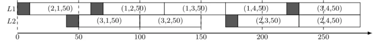
The optimal solution to this problem is given below. Figures 1 and 2 show the production and distribution plans, respectively. The former illustrates a Gantt chart showing the production and setup operations over the two lines (L1 and L2). The setups are represented by the dark gray bars. The production operations are white bars and the processing lots are given by the
Table 1: Demand (demjc) and Shelf-life (slj).
demjc C1 C2 C3 C4 slj
P 1 0 50 50 50 200 P 2 50 0 50 50 400 P 3 50 50 0 50 150
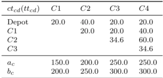
Table 2: Travel costs (ctcd) and times (ttcd) and time-windows (ac,bc).
ctcd(ttcd) C1 C2 C3 C4 Depot 20.0 40.0 20.0 20.0 C1 20.0 20.0 40.0 C2 34.6 60.0 C3 34.6 ac 150.0 200.0 250.0 250.0 bc 200.0 250.0 300.0 300.0
representation (j, c, qjlsc ), i.e., the product and the customer numbers followed by the lot size. The latter figure identifies the delivery routes taken by the vehicles. The boxed depot node D is where all the delivery operations start and circle nodes C1, C2, C3 and C4 denote the customers. The arrows represent the travel, along with the starting and completion times of the travels. When the vehicle returns to the depot, the arrow information contains the vehicle index. Table 3 complements the information of the two plans, showing some timing variables. The solution objective value is 1654.6 cost units.
L1 (1,2,25) (3,1,50) (3,2,50) (3,4,50) (2,3,50) L2 (1,2,25) (2,1,50) (2,4,50) (1,4,50) (1,3,50)
0 50 100 150 200 250
Figure 1: Production plan of the optimal solution.
The result shows that the plans were directly affected by the perishability constraints, namely the sequence order established in vehicle V 4 route and the split of the order for product 1 from customer 2. Without the perishability requirements, the optimal solution would cost 1154.6, due to two setup operations which would have been avoided. Furthermore, if the lot sizing/splitting had not been allowed, the cost of the optimal solutions would have increased. In case the products are perishable the optimal solution cost would be 1660.0, otherwise 1410.0 cost units, due to the reduction of one setup operation. So far, another interesting result lies when separate models for the production planning and distribution planning are assumed. In this case some of the coupling constraints should be revisited, and some extra assumptions should be made, affecting the flexibility created by the integration of the production and distribution planning. For instance, it is advisable to keep product’s lifespan to last beyond the customer time window for the decoupled problem, whereas the lifespan of a perishable good may last within the time
D C1 C2 C3 C4 160 180 180 200 V 1 245 265 265.4 300 V4
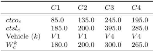
Figure 2: Distribution plan of the optimal solution. Table 3: Timing customer-dependent variables partial solution.
C1 C2 C3 C4 ctcoc 85.0 135.0 245.0 195.0
ctslc 185.0 200.0 395.0 285.0
Vehicle (k) V 1 V 1 V 4 V 4 Wck 180.0 200.0 300.0 265.0
window in the integrated model. Solving the production planning first and the distribution planning later, the overall solution is 1660 cost units, the same solution obtained when lot sizing is not allowed. Otherwise, solving the distribution planning first, the overall solution is 1654.6 cost units, the same solution to the integrated approach. In this small case, as Figure 2 shows, the distribution problem solution is straightforward. However, the solution of larger distribution problems may lead to production planning infeasibilities, as in the case that many perishable products should be produced and assigned for the same vehicle.
3
Proposed Methods
This section presents the developed methods and their parameter tuning procedures. Some traditional methods are taken into account for comparison, including: 1) the trial to solve the problem exactly using MILP-solvers; 2) the previous method with an initial solution injected to the branch-and-bound tree (also known as warm start); and 3) the traditional fix-and-optimize method, considering the customer time-windows sequence in the planning horizon. The proposed Adaptive Large Neighbourhood Search (ALNS ) is presented.
3.1
The first solution
The first solution is mandatory for both fix-and-optimize and ALNS methods. In advance, the MILP-solver may not even find a first solution in reasonable time. An initial solution may be injected to the MILP-solver to be improved by its own methods. The first solution is achieved by a constructive heuristic procedure (Heur ). The aim is to obtain a first solution in a short amount of time, allowing the improvement methods to generate better solutions. Heur states some simple rules to obtain a solution, as described in the following.
The first rule is the batching policy, i.e., a customer order for a product is entirely produced in one slot, without permitting the lot splitting. We also define that each slot should be occupied by just one order. As the number of vehicles and customers is the same (N = V ), one vehicle is assigned to each customer delivery. Moreover, we state that the delivery occurs at the end of the customer time-window. The third rule is the “first to come, first to serve” rule, that is, the customer whom has to be delivered first has its order manufactured first. Finally, the customer orders are systematically assigned to the lines, in order to perform line-assignment decisions. In this assignment, all the positive demand orders (demjc > 0) are sequenced by customer and
product order in set Π. Each order in set Π is then assigned to each line, in a linear cyclical manner, i.e., the first order is assigned to the first line, the next order is assigned to the next line (in case there is no next line, the assignment turns back to the first line), and so on until all orders have been assigned to the lines. Algorithm 1 describes the procedure of the constructive heuristic.
Algorithm 1: Constructive heuristic.
Set a sequence of customers Φ in the ascending order of the end of time-window bc
Define size of Π, π = 0 for c = {Φ1, ..., ΦN} do for j = {1, ..., P } do if demjc> 0 then π = π + 1 Ππ= (j, c) end end end Set l = 1, s = 1 for i = {Π1= (j1, c1), ..., Ππ= (jπ, cπ)} do Set qci l,ji,s= demji,ci l = l + 1 if l > L then l = 1 s = s + 1 end end for c = {1, ..., N } do xc0c= xcc,N +1= 1 wcc = bc end
From the fixed variables, determine the remaining integer variables y, z, λ, x Solve the remaining linear problem to find the timing decision variables
For instance, using the example detailed in Section 2.2, the Heur procedure runs as follows. First, the “first to come, first to serve” rule is applied, i.e., a sequence of the customers is made according to the ascending order of bc. Then, the orders are assigned to the lines. Let the
assigned to line L2, (P 1, C2) to L1 and so on, until (P 3, C4) to L1. Decisions on the sequence of the customer orders assigned to the same line are made. In this case, the sequence of orders (P 1, C4) and (P 3, C4) may be swapped in line L1. The production plan is shown in Figure 3. The distribution plan is simple, as a distinct vehicle is assigned to each customer and the delivery time is fixed by the upper bound of the customer time-windows, i.e., Wcc = bc. The solution in
Figure 3 values 2450.0 cost units.
L1 (2,1,50) (1,2,50) (1,3,50) (1,4,50) (3,4,50) L2 (3,1,50) (3,2,50) (2,3,50) (2,4,50)
0 50 100 150 200 250
Figure 3: Production plan given by the heuristic (Heur ) solution.
3.2
Traditional methods
The traditional methods considered here are deterministic approaches based on the MILP-solver. Three methods are assessed. The first two are simply the MILP-solver solutions with and without a given initial solution. The latter is the Fix-and-Optimize. This approach starts with an initial solution and proceeds by systematically fixing part of the solution and resolving the rest, in order to improve the solution in that specific neighbourhood. Many strategies can be found in the literature to best determine the sequence in which decision variables should be fixed or freed. For instance, time-based neighbourhoods are commonly developed for lot-sizing problems. In these cases, the sequences of freed neighbourhoods are chosen according to the time in which the decisions affect the solution. The fix-and-optimize approach usually relies on the strategy of overlapping neighbourhoods, i.e., intersectioned neighbourhoods with common free variables.
The fix-and-optimize procedures tested here start from the initial solution provided by the heuristic described in Section 3.1. Then, a sequence of customers based on the ascending or-der of their delivery time-windows is stated. All the binary variables related to a customer are either freed or fixed. Two parameters are necessary: the size of the free neighbourhood in each iteration and the size of the overlapping variables. We may denote the fix-and-optimize procedures by F O x y, where x is the size of the free neighbourhood and y is the number of overlapping customers. Based on this customer sequence, the procedure starts by fixing all customer-related variables except those of the x first customers. After solving this sub-problem, it fixes all customer-related variables except those of the next x customers, considering y over-lapping customers. This procedure continues until the subproblem for the last set of customers has been solved. Algorithm 2 shows the pseudo-code of this procedure. Figure 4 illustrates the fix-and-optimize procedures F O 1 0 and F O 3 1. In these examples eight customers are represented by the ellipses. The grey ones represent the customers with free variables, whereas the white customers are fixed. Each arrow separates two consecutive iterations. The arrow with the suspension points indicates that some analogous iterations are not shown. The F O x y
procedure ends after the ith iteration, which is given bylN −yx−ym. 1st 2nd 3rd lN −y x−y mth F O 1 0 1 2 3 4 5 6 7 8 1 2 3 4 5 6 7 8 1 2 3 4 5 6 7 8 ... 1 2 3 4 5 6 7 8 F O 3 1 1 2 3 4 5 6 7 8 1 2 3 4 5 6 7 8 1 2 3 4 5 6 7 8 1 2 3 4 5 6 7 8
Figure 4: Differences between F O 1 0 and F O 3 2.
Algorithm 2: Proposed fix-and-optimize heuristic (F O x y). Input: feasible solution sol
Parameters: x and y (neighbourhood size and overlap, respectively) Make a sequence of the customers seq (increasing delivery time-windows) Customer c = 1
repeat
for customer c0 from 1 to c − 1 do
Fix all variables λ and X from sol of customer seq(c0) end
for customer c0 from c + x to N do
Fix all variables λ and X from sol of customer seq(c0) end
Solve the subproblem c = c + x - y
until there are no neighbourhoods to be visited ;
3.3
The ALNS
The large neighbourhood search (LNS ) metaheuristic, proposed by Shaw (1998), aims to im-prove the solution through destroy and repair operators. Given an initial solution, the destroy operators undo part of it, removing some stated decisions. An implicit neighbourhood is created and a repair operator searches for new solutions there, inserting new decisions based on the maintained/fixed ones. The adaptive large neighbourhood search (ALNS ) is defined by Ropke and Pisinger (2006) as “an LNS heuristic that uses several competing removal and insertion heuristics and chooses between using statistics gathered during the search”. Pisinger and Ropke (2010) summarize the improvement of the LNS approach and its extensions with the key-word adaptiveness. The LNS approach has successfully solved many problems, including scheduling and transportation applications, which clearly justifies our interest. The first work, Shaw (1998), implements the LNS heuristic for the vehicle routing problem with time windows (VRPTW ). Ropke and Pisinger (2006) made it adaptive for the pickup and delivery problem. Amorim et al. (2014) also used the ALNS framework for the VRPTW, considering perishable goods,
heteroge-neous fleet and multiple time windows. Muller et al. (2012) presented a hybrid ALNS for the lot-sizing problem with setup times using an MILP-solver in the repair phase, instead of a “pure” heuristic.
Our LNS approach is adaptive and hybrid. The initial solution to the ALNS is given by the heuristic proposed in Section 3.1. Given a solution, a destroy and a repair operator are chosen adaptively. A set composed of multiple destroy operators d ∈ Ω is proposed. All destroy operators determine that some integer decision variables are fixed and the rest remain free, i.e., the destroy operators analyse the neighbourhood generated by the free decisions. The binary variables chosen to be fixed are λ and X, respectively, the production and distribution assignment variables. The single repair procedure is given by the MILP-solver restricted to a limited time. As the number of free binary variables affects the efficiency of the repair heuristic, the destroy operators may have a changing parameter σd, d ∈ Ω, bounded inferiorly and superiorly. The
adaptive parameters control the number of free variables, hence the size of the neighbourhood browsed by the repair heuristic. The current values of these parameters may be increased or decreased according to the run of the repair heuristic. In case the sub-problem is solved by the repair procedure before the limited time, or the final optimality gap is smaller than a given percentage, a larger neighbourhood may be explored and the parameter is increased. In case the final optimality gap is bigger than a given percentage, the parameter is decreased. Otherwise, σd remains unchanged. The increase or decrease in the optimality gap value may be different
according to the destroy operator. Thus, the adaptive parameters for the operators allow the ALNS to be run in distinct environments, avoiding an initial tuning of the operator parameters. The acceptance criterion, different from Ropke and Pisinger (2006), Kovacs et al. (2011) and Amorim et al. (2014) that resort to a simulated annealing framework, is simply the acceptance of the new solution in case it is better than the current. Furthermore, the best solution is always inserted as a warm start for the new search. The new solution is never worse than the current one and the search procedure becomes faster. A better new solution (newsol) means that the new solution objective function value c(newsol) is strictly lower than c(bestsol). Our solution framework requests a different strategy from the current literature regarding the weights and the scores of each destroy/repair operator. As the repair operator is unique, all the weights and scores are related to the destroy operators, hence to the combination destroy/repair operators. The probability φd of choosing a destroy operator d is proportional to the weight ρd and given
by (25). At the beginning, all probabilities φd, d ∈ Ω are set to one.
φd=
ρd
P
d0∈Ωρd0
(25)
In each iteration of the ALNS, a destroy/repair operator is chosen by the roulette wheel selection. Scores ψd, d ∈ Ω are set to zero at the beginning of the run and after every weight
update. The scores are updated after each iteration by summing up one unit to the score (ψd = ψd+ 1). As the acceptance criterion does not accept worse solutions, the score changes
only in case a new solution is found. Weights ρd, d ∈ Ω are updated every itup iterations by
(26), according to scores ψdand a parameter α, which controls the influence of new and historical
information.
ρd = (1 − α) × ρd+ α × ψd (26)
The pseudo-code of the proposed ALNS method is described in Algorithm 3. Algorithm 3: Proposed ALNS.
Input: feasible solution sol bestsol = sol
iteration it = 0 repeat
Choose destroy method d ∈ Ω using probabilities φd
Fix variables λ and X according to d and size parameter σd
newsol = M ILP (d(sol)) if c(newsol) < c(bestsol) then
bestsol = newsol update ψd
end
update σd and it
if iteration it is a multiple of itup then
update ρd, φd and ψd
end
until time limit has been reached ;
All the operators represent a neighbourhood in which a new better solution may be found. In fact, they focus on the different aspects of the solution that may be improved. As different instances are taken into account, some of the neighbourhoods may be more effective in distinct situations, as well as in different instants of the search. The adaptive parameters reward the effectiveness and success of the operators. The destroy operators and their adaptive parameters are defined in the following.
Operator Cst : This first operator aims to improve joint production and distribution decisions on customers with near time-windows. A sequence of the customers is determined according to the ascending order of their time-windows. Then, all the decisions on the chosen consecutive customers are revisited. The number of customers is adaptively chosen between 2 and N , with a (de)increment of 1.
Operators Cst-P, Cst2-P and Cst3-P : These operators are analogous to operator Cst, except that all the distribution decisions are now fixed to the values of the incumbent solution. The Cst2-P and Cst3-P operators also constrain the number of products allowed to be freed to 2 and 3 products, respectively. So, instead of freeing variables λcljs(Cst-P ), only those related to a set of randomly chosen products are freed. When the number of products allowed to have any change is lower, more customers may be involved in the decision process. These operators aim to reschedule and allow a broader neighbourhood for lot sizing/splitting decisions.
Operators Slt1-P, SltL-P, SltT-P : These operators focus on rescheduling the decisions made in different production slots. For all the operators the distribution processes are fixed. Operator Slt1-P randomly chooses some slots of the same line. The production processes present in these slots are freed. The decisions of all the other slots and lines are fixed. Operator SltL-P selects the same number of adjacent slots in each line. Differently stated, the last operator, SltT-P, sets a period of time and the decisions of all the respective slots across all the production lines are freed. Parameter σ for Slt1-P stands for the total number of slots chosen. For operator SltL-P, σ refers to the number of slots taken in each line. Finally, the changing parameter for SltT-P is the size of the time interval used to choose the slots.
Operator Dst : This last operator resolves the distribution sub-problem with all the production decisions fixed. All the vehicles-related variables are freed. This particular operator does not have any changing parameters, because its solution is quite fast.
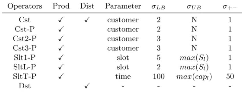
Table 4 summarizes some information of the proposed destroy operators. The first column lists the operators. The second and third columns define the type of planning decisions these operators are focused on: production (Prod) and/or distribution (Dist), respectively. The re-maining columns state how the σd parameter changes: the lower bound (σLB) and the upper
bound (σU B) of the parameter and its (de)increment (σ+−). For instance, operator Cst3-P
tack-les only the production planning and σCst3−P changes the number of customers freed in each
iteration from 3 to N customers, with (de)increments of one unit. Table 4: Destroy operators of the ALNS.
Operators Prod Dist Parameter σLB σU B σ+−
Cst X X customer 2 N 1 Cst-P X customer 2 N 1 Cst2-P X customer 3 N 1 Cst3-P X customer 3 N 1 Slt1-P X slot 5 max(Sl) 1 SltL-P X slot 2 max(Sl) 1 SltT-P X time 100 max(capl) 50 Dst X - - -
-4
Computational Results
This section tests the developed methods with a set of instances. In the following, the generation of the test instances is described. Afterwards, the computational results are shown and the developed methods are compared.
4.1
Data Generation
The instance generator presented in Amorim et al. (2013b) is extended since, to the best of our knowledge, there are no other instances for the OIPDP. Twenty combinations of number of
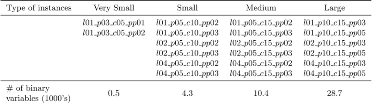
lines (L), products (P ), customers (N ) and perishable products (P∗) were generated. A compact nomenclature for the combinations is denoted by the short name lL pP cN ppP∗, given the parameters listed above. These combinations are divided into four groups, according to the number of binary variables inherent to the MILP model, which indicates the size of the problem: very small, small, medium and large. Table 5 shows all the combinations and the approximate number of binary variables. For each combination, five instances were generated, totalizing 100 instances.
Table 5: Different combinations and the approximate number of binary variables (in thousands).
Type of instances Very Small Small Medium Large
l01 p03 c05 pp01 l01 p05 c10 pp02 l01 p05 c15 pp02 l01 p10 c15 pp03 l01 p03 c05 pp02 l01 p05 c10 pp03 l01 p05 c15 pp03 l01 p10 c15 pp05 l02 p05 c10 pp02 l02 p05 c15 pp02 l02 p10 c15 pp03 l02 p05 c10 pp03 l02 p05 c15 pp03 l02 p10 c15 pp05 l04 p05 c10 pp02 l04 p05 c15 pp02 l04 p10 c15 pp03 l04 p05 c10 pp03 l04 p05 c15 pp03 l04 p10 c15 pp05 # of binary 0.5 4.3 10.4 28.7 variables (1000’s)
The rest of the parameters are drawn as follows. First, the lines are considered identical, so the parameters of a line are equal to the other lines. For all products and lines tplj= 1, cplj = 0,
mlj = 5 and αl = 1. The number of production slots of each line Sl is set to the first integer
greater or equal than P ×NL in order to ensure that all the necessary setups and deliveries are performed. 75% of the demand demjcis generated from the uniform distribution in the interval
U [40, 60] and the remaining 25% is set to zero. The setup times stblij are given by U [6, 10]
and the setup costs scblij are computed as scblij = 25.0 × stblij. There is no setup time or
cost for setups between products of the same type. The line capacity Capl is determined by:
Capl= P
jcdemjc×tplj
0.8L + max tt. We estimate that the capacity utilization of the production is
80% and the capacity is complemented with max tt as the maximum travel time. The shelf-life of the perishable products (slj) is given by min{0.3 × Capl; max tt + 75 × U [2, 3]}.
The travel times and costs are assumed to be the same. First, all customers are randomly positioned in a square of locations from (0,0) to (100,100). The depot is located at point (50,50). Then, the Euclidean distance is calculated between all pairs of customers and the depot. The service times sc are negligible. The number of available vehicles is set to N and the cost of using
each vehicle ¯f t is set to 250. The capacity of the vehicle is computed by CapV = 3×
P jcdemjc
N .
The last parameters are the time windows of each customer (parameters ac and bc), which
are calculated according to each customer orders. To generate these time windows, we propose the procedure described in Algorithm 4. The algorithm assigns each order of a customer to a line, represented by vector A, which accounts for the cumulative times of the assignments. The time windows are then generated according to the maximum time found in A, the travel time and a small amount of time to guarantee the deliveries, and to perform potentially the delivery
of multiple customers by a single vehicle. In the description of the algorithm, the maximum setup time is denoted by max stb and the value of the average demand element by av dem.
Algorithm 4: Pseudo-code to generate time windows Allocate a vector with size L and null values A[L] = [0..0]; Define a cyclical iterator it for A;
for c = 1; c <= N ; c + + do for j = 1; j <= P ; j + + do
if demjc> 0 then
Sum demjc+ max stb to A[it] ;
it + +; end end
Define aux = U [2, 8] × 0.1 × av dem; Find the maximum time on A (max(A)); Set ac= max(A) + tt0c+ aux;
Set bc= ac+ 40;
end
All the 100 instances are tested for feasibility purposes with the heuristic which generates the first solution. In case a solution is not found, then a new instance is generated until feasibility has been achieved. The instances are available at http://paginas.fe.up.pt/~pamorim/OIPDP.htm.
4.2
Results
All computational experiments were performed on a workstation with two four-core Intel Xeon E5504 at 2.00 GHz with 24 GB RAM, running Linux. CPLEX version 12.4 from IBM was used as the MILP-solver. The data generator described in Section 4.1 was used to obtain the instance set. The maximum computational time for all methods was 3600 seconds. The MILP-solver was set to the maximum of 4 threads, opportunistic mode, across the methods.
Due to the strong NP-hardness of the OIPDP (Amorim et al., 2013b), it is not possible to find even integer solutions to the small instances with MILP-solvers. Therefore, we relied on the constructive heuristic to obtain the first solutions. These solutions were used as a starting point for the OIPDP, i.e., they were injected into the branch-and-bound tree of the MILP-solver.
Three parameters needed to be set for the ALNS : 1) operator time; 2) parameter α, which defines a proportion for the historical and new weights; and 3) parameter itup, which determines
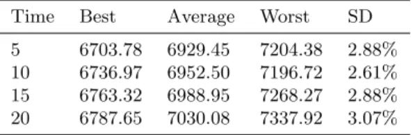
the frequency at which the weights are updated. The latter parameter was fixed to 20 iterations. Each operator has a limited time to destroy and repair the solution. As operator Cst performs a search in the integrated environment, it is given 5 more seconds than the other operators, which have the same time limit. To find out the better time limit, some tests were performed considering α = 0, i.e., the operators have always the same probability to be chosen. The operator times of 5, 10, 15 and 20 seconds were tested and the results are shown in Table 6. The columns denote the
best, average and worst results for all instances, respectively, and the standard deviation (SD) of the quality of the solution, which measures the robustness of the method. Giving 5 seconds to each operator seems to deliver the best performance: the ALNS gets better as the number of iterations increases. We then tested the influence of parameter α, considering the 5 second limit for each operator. Parameter α is important to establish the weights and probability of an operator being chosen. A higher α implies a strategy more focused on the intensification, whereas a smaller α aims to diversify the solution. Table 7 shows the respective results. The columns are analogous to those of Table 6. The results show that a balanced value for α yielded the best average performance. So, the experiments indicate that the best configuration for the ALNS is to consider 5 seconds time limit for operators, α = 0.2 and itup= 20.
Table 6: Results for the ALNS with different operator time limits.
Time Best Average Worst SD
5 6703.78 6929.45 7204.38 2.88%
10 6736.97 6952.50 7196.72 2.61%
15 6763.32 6988.95 7268.27 2.88%
20 6787.65 7030.08 7337.92 3.07%
Table 7: Results for the ALNS with different α values.
α Best Average Worst SD
0.0 6703.78 6929.45 7204.38 2.88% 0.2 6710.81 6920.88 7186.87 2.91% 0.4 6749.47 6974.33 7228.49 2.85% 0.6 6761.19 7029.31 7362.38 3.35%
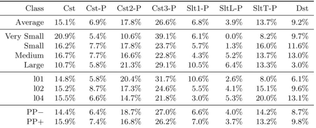
For this ALNS configuration, Table 8 shows the relative frequency of the number of improve-ments obtained by each destroy/repair operators along each run of the algorithm. The results are clustered regarding the different classes of instances. The first row depicts the overall average performance. The instances are then split by size: very small, small, medium and larger, num-ber of lines and numnum-ber of perishable products: PP− and PP+, which agreggate the instances from each type that have less and more perishable products, respectively. Operators Cst3-P and Cst2-P are the most effective, being responsible for 26.6% and 17.8% of the improvements, respectively. The improvements obtained by these operators are more significant than the ones delivered by operator Cst-P (6.9%), which is also concerned about the neighbourhood of pro-duction decisions of different customers with fixed distribution, though the number of products taken into account by operator Cst-P is not constrained. It seems more interesting to tackle each partition with more customers together with a limited number of items. It is worth of mention that the performance of the operators are dependent on its sequence throughout the search. Table 8 also presents some characteristics of the operators according to the problem parameters. Operator Cst, which allows for joint decisions on the production and distribution
planning, is negatively affected by the increase of the number of products, as the size of the neighbourhoods and the number of customer-related free variables increase. The opposite occurs with Cst2-P and Cst3-P operators, whose effectiveness in achieving better solutions is improved, as the number of products is fixed. Notice that, for very small sized instances, the performance of operators Cst-P and Cst3-P is similar. The slot-strategy operators are more affected by the number of lines. Moreover, operator Slt1-P seems more suitable for problems with fewer lines, as it chooses only one line each iteration to re-optimize the production planning decisions and, therefore, line assignment decisions are not modified. The same arguments apply for the opposite behaviour of operator SltT-P. With more lines and the same number of products and customers, the customer time-windows tend to be closer, expanding the solution space of the distribution planning and, potentially improving the performance of the operator Dst. This operator is also affected by the number of products as a larger product portfolio incurs in more production de-cisions. Finally, the number of perishable products has a small influence on the performance of the operators (the performance difference was never larger than 2%). In fact, there was no need for perishable-driven operators, since the current operators handle the operations with this type of products.
Table 8: Performance evaluation of the operators of the ALNS.
Class Cst Cst-P Cst2-P Cst3-P Slt1-P SltL-P SltT-P Dst Average 15.1% 6.9% 17.8% 26.6% 6.8% 3.9% 13.7% 9.2% Very Small 20.9% 5.4% 10.6% 39.1% 6.1% 0.0% 8.2% 9.7% Small 16.2% 7.7% 17.8% 23.7% 5.7% 1.3% 16.0% 11.6% Medium 16.7% 7.7% 16.6% 22.8% 4.3% 5.2% 13.7% 13.0% Large 10.7% 5.8% 21.3% 29.1% 10.5% 6.4% 13.3% 3.0% l01 14.8% 5.8% 20.4% 31.7% 10.6% 2.6% 8.0% 6.1% l02 15.2% 8.7% 17.3% 24.6% 5.5% 4.1% 15.1% 9.6% l04 15.5% 6.6% 14.7% 21.8% 3.0% 5.3% 20.0% 13.1% PP− 14.4% 6.4% 18.7% 27.0% 6.6% 4.0% 14.2% 8.7% PP+ 15.9% 7.4% 16.8% 26.2% 7.0% 3.7% 13.2% 9.8%
Six fix-and-optimize configurations were tested: FO 1 0, FO 2 0, FO 2 1, FO 3 0, FO 3 1 and FO 3 2 (see Section 3.2 for the difference between these methods). The configurations were compared using the solution performance gap, i.e., the difference between the incumbent solution objective value of each method and the best solution achieved by the methods compared, divided by the same best solution. The best results were achieved by configurations FO 3 1 and FO 3 2, with an average solution performance gap of 4.03% and 3.14%, respectively. The most successful fix-and-optimize methods include only the procedures with overlapping, which shows the success of this feature. Larger neighbourhoods (three costumers optimized per iteration instead of less costumers) lead to better solutions on average.
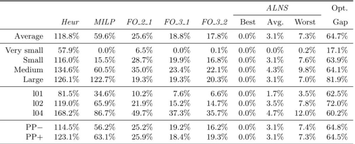
We then benchmark the performance of ALNS against the other solution methods. Table 9 provides the average solution performance gaps of the best methods and the optimality gap of the
best solution achieved and the lower bound provided by the MILP-solver. The rows are analogous to Table 8 and denote the parameters of the instances. The first columns report the upper-bound given by the construction heuristic (Heur ), MILP-solver (MILP ), fix-and-optimize approaches and ALNS. As the ALNS is not deterministic, which influences the algorithm performance, we have run the ALNS five times for each instance with different random seeds and report the best, average and worst results. The last column depicts the optimality gap of the best solution obtained across all methods. Table 9 indicates that the ALNS method yielded the best results, with a large difference over the other methods and the best run of ALNS achieved the best solu-tions for all instances. The heuristic provides poor-quality solusolu-tions and the MILP performance is strongly affected by the size of the problem, number of lines and perishable items. Fix-and-optimize methods with larger neighbourhoods obtained a competitive performance compared to MILP, with better results for medium to large instances. The average solution performance gap show that even the incumbent solution found in the worst run of the ALNS method is better than the solutions achieved by the other methods, for most of the cases. Nine in ten runs of ALNS yielded better solutions than the other methods and the best solution value found by the
traditional procedures were 12.7% greater than ALNS, on average. The average optimality gap
presented is large even for very small instances.
Table 9: Average solution performance gap and the best optimality gap achieved.
ALNS Opt.
Heur MILP FO 2 1 FO 3 1 FO 3 2 Best Avg. Worst Gap
Average 118.8% 59.6% 25.6% 18.8% 17.8% 0.0% 3.1% 7.3% 64.7% Very small 57.9% 0.0% 6.5% 0.0% 0.1% 0.0% 0.0% 0.2% 17.1% Small 116.0% 15.5% 28.7% 19.9% 16.8% 0.0% 3.1% 7.6% 63.9% Medium 134.6% 60.5% 35.0% 23.4% 22.1% 0.0% 4.3% 9.8% 64.1% Large 126.1% 122.7% 19.3% 19.3% 20.3% 0.0% 3.1% 7.0% 81.9% l01 81.5% 34.6% 10.2% 7.6% 6.6% 0.0% 1.7% 3.5% 62.5% l02 119.0% 65.9% 21.9% 15.2% 14.7% 0.0% 3.5% 7.8% 72.0% l04 168.2% 86.7% 49.7% 37.3% 35.7% 0.0% 4.7% 12.0% 60.2% PP− 114.5% 56.2% 25.2% 19.2% 16.2% 0.0% 3.1% 7.4% 64.8% PP+ 123.1% 63.1% 25.9% 18.4% 19.3% 0.0% 3.1% 7.3% 64.5%
In order to have an overall perspective of the benchmark, we compare the methods using performance profiles (Dolan and Mor´e, 2002). In these performance profiles, we can choose procedures (s ∈ S) to be evaluated by a set of instances (p ∈ P) using a performance measure (t), which, in our case, is the objective function. For each instance p, the smallest objective function value obtained by the compared methods becomes the reference for the performance ratio rp,s given by (27). Now, ρs(τ ) : τ ≥ 0 is defined as the proportion of instances solved
by method s with performance ratio lower than or equal to τ . The chart represents function ρs(τ ), which is the (cumulative) distribution function for the performance ratio (Dolan and Mor´e,
rp,s= tp,s− min {tp,s : s ∈ S} min {tp,s : s ∈ S} (27) ρs(τ ) = |p ∈ P : rp,s ≤ τ | |P| (28)
Figure 5 illustrates the performance profile comparing the heuristic proposed in Section 3.1 (Heur ), the MILP-solver with the heuristic solution as the initial solution, the fix-and-optimize variants (FO 2 1, FO 3 1 and FO 3 2 ) and the ALNS. The chart shows the performance of the methods regarding the solution value (rp,s is the value of the solution achieved by method s in
instance p). In the chart, τ ranges from 0% to 100% (τ ∈ [0, 1]), i.e., all the solutions worse than at least 2 times the best solution found are neglected. To infer the performance of the ALNS we use the grey area that is limited by the best and worst cases of the five test runs and we also depict the average run. The ALNS showed a superior performance, as the best run always achieved the best solution to P. Moreover, the worst runs of the ALNS beat the other methods. The FO 3 1 and FO 3 2 fix-and-optimize methods had similar performance, better than the FO 2 1. The MILP solution is far from the best solution achieved. Naturally, the worst performance belongs to the constructive heuristic method. However, the aim of the heuristic is to provide a fast solution, commonly a solution with a poor quality, given the assumptions taken by the heuristic. The Heur and MILP procedures have 37% and 73% of their solutions with rp,s ≤ 100%. The other methods always found a solution within τ = 100%. The worst ALNS
case has a solution with a relative difference of 35.1% from the best solution found. For example, the MILP has 45% of the solutions with a performance within the same value (τ = 35.1%).
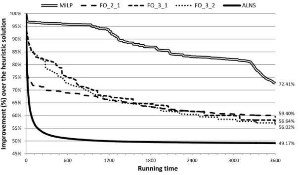
Figure 6 shows a comparison of the methods concerning the improvement in the solution along the running time. The improvement of a solution is measured relative to the heuristic solution, which is the common warm start for all the compared methods. The ALNS solution value is given by the average. For each method the overall average improvement at the end of the search is shown. The chart clearly highlights the better performance of the ALNS method, mainly at the beginning of the run. Although the improvement in the MILP solution is slower, in the end it becomes faster, probably due to the MILP-solver strategy. The fix-and-optimize methods show a similar behaviour, however the FO 2 1 shows a better performance in the beginning, as it deals with smaller neighbourhoods. Notice that the neighbourhoods of the FO 2 1 are also considered in the ALNS by operator Cst. This comparison reinforces the statement that the use of different neighbourhoods may result in longer improvements.
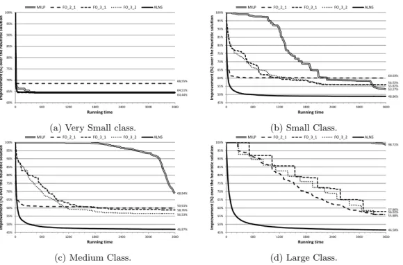
Figure 7 details the benchmark by plotting the performance of the average solution value relative to the warm start solution in time for the four classes of instances: very small (7a), small (7b), medium (7c) and larger (7d). For the very small class, the proposed methods show similar performance, achieving the final solution in a short period of time. For the remaining cases, there is an unquestionable dominance of the ALNS over the other procedures. Averagely, even the worst run of the ALNS outperformed the other approaches (see Table 9). The ALNS convergence
0% 10% 20% 30% 40% 50% 60% 70% 80% 90% 100% 0% 10% 20% 30% 40% 50% 60% 70% 80% 90% 100% Cumul ati ve d ist rib uti on 𝜌 s (𝜏 ) Deviation (𝜏)
Heur MILP FO_2_1 FO_3_1 FO_3_2 ALNS
Figure 5: Performance evaluation of the proposed methods.
72.41% 59.40% 56.64% 56.02% 49.17% 45% 50% 55% 60% 65% 70% 75% 80% 85% 90% 95% 100% 0 600 1200 1800 2400 3000 3600 Imp ro ve men t (%) o ve r th e h eu ri sti c so lu ti o n Running time
MILP FO_2_1 FO_3_1 FO_3_2 ALNS
gets slower as the size of the instances increase, however the difference of the ALNS solutions to the other method solutions is augmented. The fix-and-optimize methods have an intermediate performance and, for larger instances, have shown a stair pattern, mainly for FO 3 1 and FO 3 2, which means that the subproblems are not solved to optimality. The performance of the MILP-solver deteriorates significantly with the size of the problem, number of production lines and perishable products. From all tested instances, the MILP-solver has only found two provably optimal solutions to instances of the very small size class. Regardless of the instance class, the optimality gap given by the relative difference of the integer solution and the lower bound of the branch-and-bound tree is large. Even the very small size class showed an optimality gap of approximately 17,1% for most of the solution methods. The number of products and customers increase this gap, contrarily to the number of lines and perishable products. These results were expected as the mathematical model is based on the well-known general lot-sizing and scheduling problem formulation (Fleischmann and Meyr, 1997), which enables the incorporation of details at the cost of delivering a weaker lower bound.
64,44% 68,55% 64,51% 60% 65% 70% 75% 80% 85% 90% 95% 100% 0 600 1200 1800 2400 3000 3600 Imp ro ve men t (%) o ve r th e h eu ri sti c so lu ti o n Running time
MILP FO_2_1 FO_3_1 FO_3_2 ALNS
(a) Very Small class.
53.27% 60.03% 56.02% 55.82% 48.86% 45% 50% 55% 60% 65% 70% 75% 80% 85% 90% 95% 100% 0 600 1200 1800 2400 3000 3600 Im prov e m e nt (%) o ve r the he uri sti c so luti o n Running time
MILP FO_2_1 FO_3_1 FO_3_2 ALNS
(b) Small Class. 68,94% 59,91% 58,76% 56,53% 46,97% 45% 50% 55% 60% 65% 70% 75% 80% 85% 90% 95% 100% 0 600 1200 1800 2400 3000 3600 Improvemen t (%) o ver the he u ri st ic soluti o n Running time
MILP FO_2_1 FO_3_1 FO_3_2 ALNS
(c) Medium Class. 98.72% 56.02% 57.80% 55.88% 46.58% 45% 50% 55% 60% 65% 70% 75% 80% 85% 90% 95% 100% 0 600 1200 1800 2400 3000 3600 Imp ro ve men t (%) o ve r th e h eu ri sti c so lu ti o n Running time
MILP FO_2_1 FO_3_1 FO_3_2 ALNS
(d) Large Class.
Figure 7: Performance of the average solution value relative to the warm start solution in time, for different instance sizes.
Table 10 shows the mean computational times of the compared methods in seconds. The proposed heuristic achieves the result in less than one second. In general, MILP-solver and ALNS have computational times greater than 3600 seconds. The fix-and-optimize methods depend on the size of the neighbourhood of each iteration. Thus, very small instances are solved faster than the larger instances. The table also indicates that instances with more perishable
products are solved faster on average. With less perishable products, the number of distinct schedule solutions are greater, unlike when there are more perishable products, which reduces the flexibility of the schedule solutions.
Table 10: Average computational times of the best methods.
Heur MILP FO 2 1 FO 3 1 FO 3 2 ALNS
Average 0.35 3547.91 1483.27 2011.09 2317.99 3600.03 Very small 0.10 3077.26 1.02 9.19 8.39 3600.00 Small 0.16 3600.06 457.51 1011.65 2055.43 3600.01 Medium 0.23 3600.11 915.38 2088.62 2077.35 3600.02 Large 0.73 3600.46 3571.00 3600.30 3591.04 3600.08 l01 0.29 3469.47 1615.20 2092.42 2397.72 3600.03 l02 0.37 3600.21 1554.41 2352.82 2902.50 3600.04 l04 0.39 3600.21 1236.22 1560.92 1627.17 3600.04 PP− 0.37 3553.35 1724.20 2083.02 2406.09 3600.03 PP+ 0.32 3542.48 1242.33 1939.16 2229.88 3600.03
5
Conclusions
In this study, we consider the operational integrated production and distribution planning prob-lem (OIPDP ) with perishable products. In the production planning, the decision-maker tackles scheduling, line-assignment and lot sizing/splitting decisions. The distribution planning consists of a vehicle-routing problem with time-windows. Besides, the perishability is a hard constraint to the problem, which reinforces the joint planning of the production and distribution operations. The OIPDP is a very difficult problem, and so far unsolvable using exact methods even for prob-lems with a small number of products and customers. An adaptive large neighbourhood search fed with a simple constructive heuristic is proposed here. This solution method is compared to some traditional approaches, as the MILP-solver limited by time and a fix-and-optimize with overlap based on customer decisions.
The ALNS outperformed the traditional methods, proving that approaches with clever adap-tive intensification and diversification procedures may lead to good solutions, even for hard problems. The ALNS improvement speed is faster than the other approaches, obtaining better results in short running times for the instances generated. A point of paramount importance on the development of the ALNS heuristic is that, in general, the bigger the number of iterations, the better the heuristic performs. Thus, small time local searches (5 seconds) were chosen and the sizes of the explored neighbourhoods were chosen adaptively, which improved the solutions achieved and the robustness of the proposed method, regardless the instance size. The various operators play a main role as they promote a search in different neighbourhoods resulting in good robust solutions.
Extensions of the OIPDP may include split deliveries and multiple customer time-windows. The problem can also be extended to consider a multi-period planning horizon and facing some tactical decisions. Such extension approximates OIPDP to the well-known inventory routing and production routing problems. As the products are perishable, the integration of the production planning with the resource planning is highly recommendable, guaranteeing good raw materials and final products with a better quality and more possibilities for decreasing the distribution costs. So far, the ALNS technique has been very flexible and destroy/repair operators may be easily manipulated for extended/closer problems, which makes the approach a suitable proposal of solution method for these problems.
References
Amorim, P., Meyr, H., Almeder, C., and Almada-Lobo, B. (2013a). Managing perishability in production-distribution planning: a discussion and review. Flexible Services and Manufactur-ing Journal, 25(3):389–413.
Amorim, P., Parragh, S. N., Sperandio, F., and Almada-Lobo, B. (2014). A rich vehicle routing problem dealing with perishable food: a case study. TOP, 22(2):489–508.
Amorim, P. S., Belo-Filho, M. A. F., Toledo, F. M. B., Almeder, C., and Almada-Lobo, B. (2013b). Lot sizing versus batching in the production and distribution planning of perishable goods. International Journal of Production Economics, 146(1):208–218.
Armstrong, R., Gao, S., and Lei, L. (2008). A zero-inventory production and distribution problem with a fixed customer sequence. Annals of Operations Research, 159(1):395–414.
Bilgen, B. and Ozkarahan, I. (2004). Strategic tactical and operational production-distribution models: a review. International Journal of Technology Management, 28(2):151–171.
Buer, M. V., Woodruff, D., and Olson, R. (1999). Solving the medium newspaper produc-tion/distribution problem. European Journal of Operational Research, 115(2):237–253. Cai, X., Chen, J., Xiao, Y., and Xu, X. (2008). Product selection, machine time allocation, and
scheduling decisions for manufacturing perishable products subject to a deadline. Computers & Operations Research, 35(5):1671–1683.
Chen, H.-K., Hsueh, C.-F., and Chang, M.-S. (2009). Production scheduling and vehicle rout-ing with time windows for perishable food products. Computers & Operations Research, 36(7):2311–2319.
Chen, Z.-L. (2004). Integrated production and distribution operations: Taxonomy, models, and review. In Simchi-Levi, D., Wu, S., and Shen, Z.-J., editors, Handbook of Quantitative Supply Chain Analysis: Modeling in the E-Business Era, volume 74 of International Series in Operations Research & Management Science, pages 711–745. Springer US.
Chen, Z.-L. (2009). Integrated Production and Outbound Distribution Scheduling: Review and Extensions. Operations Research, 58(1):130–148.
Dolan, E. D. and Mor´e, J. J. (2002). Benchmarking optimization software with performance profiles. Mathematical Programming, 91(2):201–213.
Entrup, M., G¨unther, H., Van Beek, P., Grunow, M., and Seiler, T. (2005). Mixed-Integer Linear Programming approaches to shelf-life-integrated planning and scheduling in yoghurt production. International Journal of Production Research, 43(23):5071–5100.
Ereng¨u¸c, S., Simpson, N., and Vakharia, A. J. (1999). Integrated production/distribution planning in supply chains: An invited review. European Journal of Operational Research, 115(2):219–236.
Fleischmann, B. and Meyr, H. (1997). The general lotsizing and scheduling problem. OR Spectrum, 19(1):11–21.
Garcia, J. and Lozano, S. (2004). Production and vehicle scheduling for ready-mix operations. Computers & Industrial Engineering, 46(4):803–816.
Garcia, J. and Lozano, S. (2005). Production and delivery scheduling problem with time windows. Computers & Industrial Engineering, 48(4):733–742.
Geismar, H. N., Laporte, G., Lei, L., and Sriskandarajah, C. (2008). The Integrated Production and Transportation Scheduling Problem for a Product with a Short Lifespan. INFORMS Journal on Computing, 20(1):21–33.
Goetschalckx, M., Vidal, C. J., and Dogan, K. (2002). Modeling and design of global logistics systems: A review of integrated strategic and tactical models and design algorithms. European Journal of Operational Research, 143(1):1–18.
Karaesmen, I. Z., Scheller-Wolf, A., and Deniz, B. (2011). Managing perishable and aging inventories: Review and future research directions. In Kempf, K. G., Keskinocak, P., and Uzsoy, R., editors, Planning Production and Inventories in the Extended Enterprise, volume 151 of International Series in Operations Research & Management Science, pages 393–436. Springer US.
Kopanos, G. M., Puigjaner, L., and Georgiadis, M. C. (2010). Optimal Production Schedul-ing and Lot-SizSchedul-ing in Dairy Plants: The Yogurt Production Line. Industrial & EngineerSchedul-ing Chemistry Research, 49(2):701–718.
Kovacs, A. a., Parragh, S. N., Doerner, K. F., and Hartl, R. F. (2011). Adaptive large neigh-borhood search for service technician routing and scheduling problems. Journal of Scheduling, 15(5):579–600.
Millard, D. (1959). Industrial inventory models as applied to the problem of inventorying whole blood. PhD thesis, The Ohio State University.
Muller, L. F., Spoorendonk, S., and Pisinger, D. (2012). A hybrid adaptive large neighborhood search heuristic for lot-sizing with setup times. European Journal of Operational Research, 218(3):614–623.
Nahmias, S. (1982). Perishable inventory theory: a review. Operations research, 30(4):680–708. Pisinger, D. and Ropke, S. (2010). Large neighborhood search. In Gendreau, M. and Potvin, J.-Y., editors, Handbook of Metaheuristics, volume 146 of International Series in Operations Research & Management Science, pages 399–419. Springer US.
Ropke, S. and Pisinger, D. (2006). An Adaptive Large Neighborhood Search Heuristic for the Pickup and Delivery Problem with Time Windows. Transportation Science, 40(4):455–472. Sarmiento, A. M. and Nagi, R. (1999). A review of integrated analysis of production-distribution
systems. IIE transactions, 31(11):1061–1074.
Schmid, V., Doerner, K. F., and Laporte, G. (2013). Rich routing problems arising in supply chain management. European Journal of Operational Research, 224(3):435–448.
Shaw, P. (1998). Using constraint programming and local search methods to solve vehicle routing problems. In Maher, M. and Puget, J.-F., editors, Principles and Practice of Constraint Programming - CP98, volume 1520 of Lecture Notes in Computer Science, pages 417–431. Springer Berlin Heidelberg.
Vidal, C. J. and Goetschalckx, M. (1997). Strategic production-distribution models: A criti-cal review with emphasis on global supply chain models. European Journal of Operational Research, 98(1):1–18.
Viergutz, C. and Knust, S. (2014). Integrated production and distribution scheduling with lifespan constraints. Annals of Operations Research, 213(1):293–318.