Corporate credit risk modeling

Texto

(1)Instituto Superior de Ciências do Trabalho e da Empresa Departamento de Contabilidade e Finanças. CORPORATE CREDIT RISK MODELING. João Eduardo Dias Fernandes Tese submetida como requisito parcial para obtenção do grau de Doutor em Gestão Especialidade Finanças Orientador: Prof. Doutor Miguel Almeida Ferreira. [Dezembro, 2006].

(2) Instituto Superior de Ciências do Trabalho e da Empresa Departamento de Contabilidade e Finanças. CORPORATE CREDIT RISK MODELING. João Eduardo Dias Fernandes Tese submetida como requisito parcial para obtenção do grau de Doutor em Gestão Especialidade Finanças Orientador: Prof. Doutor Miguel Almeida Ferreira. [Dezembro, 2006].

(3) C O R PO R A T E C R E D IT R ISK M O D E L IN G João E duardo D . F ernandes.

(4) Agradecimentos. Gostaria de agradecer em primeiro lugar ao Banco BPI, SA e, em particular ao Dr. Rui Martins do Santos por possibilitarem a utilização de dados e recursos internos para este trabalho de investigação. Um agradecimento especial ao Prof. Miguel Almeida Ferreira pelo apoio e orientação. Gostaria igualmente de agradecer a todas as pessoas que contactei ao longo destes últimos 4 anos pelo apoio e comentários da maior relevância. Em particular agradeço aos meus colegas Drs. Jorge Barros Luís, Luís Ribeiro Chorão, Carla Cavaco Martins, Dária Adriano Marques, Isabel Moutinho e Yuneza Abdul Latif, e à Prof. Cristina Neto de Carvalho da Universidade Católica Portuguesa. Pelo encorajamento e paciência agradeço e dedico este trabalho aos meus pais e irmão e à minha Carla. Por último gostaria de deixar uma palavra de agradecimento à FCT – Fundação para a Ciência e Tecnologia pelo apoio financeiro prestado a este projecto.. i.

(5) Resumo. A modelização do risco de crédito de empréstimos a empresas sem emissões cotadas em mercados financeiros é limitada, apesar do peso elevado deste segmento nas carteiras de crédito dos bancos. O objectivo deste estudo é contribuir para este ramo de literatura ao aplicar técnicas de medição dos dois principais parâmetros de risco de crédito a uma amostra aleatória extraída da base de dados de um banco europeu. A dissertação é composta por dois capítulos, o primeiro trata a modelização da probabilidade de incumprimento (PD), e o segundo a modelização da perda em caso de incumprimento (LGD). O primeiro capítulo começa por apresentar e comparar alternativas para a medição do credit score dos clientes, incluindo modelo de equações sectoriais múltiplas e outro com amostra ponderada. Em seguida é abordada a problemática de agrupar scores individuais em classes de risco com PDs associadas. Para tal, duas alternativas são propostas, a primeira usa técnicas de clustering, enquanto que a segunda baseia-se no mapeamento entre as classificações internas e uma escala de referência externa. No final do primeiro capítulo, e usando as estimativas de PD anteriormente calculadas, determinam-se os requisitos de capital regulamentar à luz do novo acordo de capital de Basileia, em contraste com os requisitos previstos no acordo actual. No segundo capítulo comparam-se duas alternativas para a modelização do LGD. Os modelos são estimados sob uma amostra aleatória de 7 anos, considerando-se como variáveis explicativas características dos empréstimos, garantias e clientes. Ambas as alternativas têm em consideração o facto da variável dependente ser uma fracção e de ter uma distribuição não normal. A primeira alternativa é baseada na transformação Beta da variável dependente, enquanto que a segunda é baseada em Generalized Linear Models. Palavras-Chave: Risco de Crédito, Probabilidade de Incumprimento, Perda em Caso de Incumprimento, Basileia II Classificação JEL: C13, G21 ii.

(6) Abstract. Corporate credit risk modeling for privately-held firms is limited, although these firms represent a large fraction of the corporate sector worldwide. This study is an empirical application of credit scoring and rating techniques to a unique dataset on private firms bank loans of a European bank. It is divided in two chapters. The first chapter is concerned with modeling the probability of default. Several alternative scoring methodologies are presented, validated and compared. These methodologies include a multiple industry model, and a weighted sample model. Furthermore, two distinct strategies for grouping the individual scores into rating classes with PDs are developed, the first uses cluster algorithms and the second maps internal ratings to an external rating scale. Finally, the regulatory capital requirements under the New Basel Capital Accord are calculated for a simulated portfolio, and compared to the capital requirements under the current regulation. On the second chapter, we model long-term Loss-Given-Default on loan, guarantee and customer characteristics using a random, 7-year sample. Two alternative modeling strategies are tested, taking in consideration the highly non-normal shape of the recovery rate distribution, and a fractional dependent variable. The first strategy is based on Beta transformation of the dependent variable, while the second is based on Generalizes Linear Models. The methodology can be used for long-term LGD prediction of a corporate bank loan portfolio and to comply with the New Basel Capital Accord Advanced Internal Ratings Based approach requirements.. KEYWORDS: Credit Risk, Probability of Default, Loss-Given-Default, Basel II JEL CLASSIFICATION: C13, G21. iii.

(7) Contents. Agradecimentos.............................................................................................................i Resumo..........................................................................................................................ii Abstract....................................................................................................................... iii Contents .......................................................................................................................iv List of Tables ..............................................................................................................vii List of Figures..............................................................................................................ix Chapter I - Quantitative Rating System And Probability Of Default Estimation 1. Introduction..........................................................................................................1. 2. Data Description...................................................................................................5. 3. Financial Ratios and Bivariate Analysis ............................................................9. 4. Scoring Model and Validation ..........................................................................14 4.1. Model Validation .........................................................................................14. 4.1.1 Efficiency.................................................................................................15 4.1.2 Statistical Significance.............................................................................17 4.1.3 Economic Intuition...................................................................................19. 5. 4.2. Model A – Multiple Industry Equations Model...........................................20. 4.3. Model B – Standard Model..........................................................................22. 4.4. Model C – Weighted Sample Model ...........................................................23. 4.5. Analysis of the Results.................................................................................26. Applications ........................................................................................................33 5.1. Quantitative Rating System and Probability of Default Estimation ............33. 5.1.1 Cluster Methodology ...............................................................................34 5.1.2 Historical / Mapping Methodology..........................................................38 5.1.3 Rating Matrixes and Stability ..................................................................41 5.2 6. Regulatory Capital Requirements ................................................................44. Conclusion ..........................................................................................................46 iv.

(8) Bibliography ...............................................................................................................48 Appendix 1 – Description of Financial Ratios and Accuracy Ratios ....................53 Appendix 2 – Estimating and Comparing the Area Under the ROC curves .......54 Appendix 3 – Binomial Logistic Regression Estimation and Diagnostics ............56 Appendix 4 – Estimation Results..............................................................................63 Appendix 5 – Kolmogorov-Smirnov and Error Type Analysis .............................67 Appendix 6 – K-Means Clustering ...........................................................................71 Appendix 7 – IRB RWA and Capital Requirements for Corporate Exposures ..72 Appendix 8 - IRB Capital Requirements Figures...................................................74 Chapter II - Loss Given Default Estimation 1. Introduction........................................................................................................78. 2. Sample Description ............................................................................................81. 3. LGD Definition...................................................................................................83. 4. Recovery Drivers................................................................................................87 4.1. Guarantee Characteristics ............................................................................88. 4.1.1 Guarantee Type...........................................................................................88 4.2. Loan Characteristics.....................................................................................89. 4.2.1 Loan Value..................................................................................................89 4.2.2 Loan Maturity .............................................................................................90 4.2.3 Default-to-Loan Value and Seasoning-to-Loan Maturity Ratios................91 4.2.4 Interest Rate ................................................................................................93 4.3. Customer Characteristics .............................................................................94. 4.3.1 Firm Industry ..............................................................................................94 4.3.2 Age of Relationship ....................................................................................95 4.3.3 Firm Age .....................................................................................................95 4.3.4 Geographic Location...................................................................................96 5. 6. LGD Modeling....................................................................................................98 5.1. Beta Transformation Methodology..............................................................99. 5.2. GLM Methodology ....................................................................................103. Conclusion ........................................................................................................107 v.

(9) Bibliography .............................................................................................................109 Appendix 1 – Kaplan Meier Survival Analysis .....................................................111 Appendix 2 – Industry Groups by Economic Activity .........................................112 Appendix 3 – Regression Fit Analysis....................................................................113. vi.

(10) List of Tables. Chapter I Table 1 – Estimated Model Variables and Parameters, Model (A) .............................21 Table 2 – Estimated Model Variables and Parameters, Model (B) .............................22 Table 3 – Estimated Model Variables and Parameters, Model (C) .............................25 Table 4 – AUROC, AR and KS Statistics....................................................................30 Table 5 – Testing the Differences between AUROC’s................................................30 Table 6 – Calinski-Harabasz CH(k) index for k = 2 up to k = 20................................35 Table 7 – Annual Global Issuer-Weighted Default Rate Descriptive Statistics, 19202003..............................................................................................................................38 Table 8 – Model A 1 Year Transition Matrix (Cluster Method) .................................42 Table 9 – Model B 1 Year Transition Matrix (Cluster Method)..................................42 Table 10 – Model C 1 Year Transition Matrix (Cluster Method)................................42 Table 11 – Model A 1 Year Transition Matrix (Historical Method) ...........................42 Table 12 – Model B 1 Year Transition Matrix (Historical Method) ...........................43 Table 13 – Model C 1 Year Transition Matrix (Historical Method) ...........................43 Table 14 – Average RWA and Total Capital Requirements........................................45. Chapter II Table 15 – Sample Distribution by Original Loan Maturity........................................81 Table 16 – Cumulative Recovery Rate Summary Statistics ........................................86 Table 17 – List of Explanatory Variables ....................................................................87 Table 18 – Guarantee Weight and Recovery Rate by Guarantee Type .......................89 Table 19 – Loan Value Summary Statistics, in EUR...................................................90 Table 20 – Loan Frequency and Recovery Rate by Loan Maturity.............................91 Table 21 – Default-to-Loan Value and Seasoning-to-Maturity Ratios Summary Statistics .......................................................................................................................93. vii.

(11) Table 22 – Loan Frequency and Recovery Rate by Interest Rate................................93 Table 23 – Loan Frequency and Recovery Rate by Industry Group ...........................94 Table 24 – Age of Relationship Summary Statistics, in Years....................................95 Table 25 – Loan Frequency and Recovery Rate by Age of Relationship....................95 Table 26 – Firm Age Summary Statistics, in Years.....................................................96 Table 27 – Loan Frequency and Recovery Rate by Firm Age ....................................96 Table 28 – Loan Frequency and Recovery Rate by Geographic Location ..................97 Table 29 – Beta Fit Descriptive Statistics..................................................................100 Table 30 – Maximum-Likelihood estimates of long-term cumulative recovery rates, Beta Methodology......................................................................................................101 Table 31 – Maximum-Likelihood estimates of long-term cumulative recovery rates, GLM Methodology ....................................................................................................105 Table 32 – Industry Groups by Economic Activity Classification ............................112. viii.

(12) List of Figures. Chapter I Figure 1 – Economy-Wide vs. Main Sample Industry Distribution ..............................6 Figure 2 – Sample Industry Distribution .......................................................................7 Figure 3 – Accounting Statement Yearly Distribution ..................................................7 Figure 4 – Size (Turnover) Distribution, Millions of EUR ...........................................8 Figure 5 – Average Default Frequency by Liquidity / Current Liabilities Ratio Decile9 Figure 6 – Average Default Frequency by Current Ratio Decile ................................10 Figure 7 – Average Default Frequency by Liquidity / Assets Ratio Decile .................10 Figure 8 – Average Default Frequency by Debt Service Coverage Ratio Decile .......11 Figure 9 – Average Default Frequency by Interest Costs / Sales Ratio Decile ...........11 Figure 10 – Average Default Frequency by Productivity Ratio Decile.......................12 Figure 11 – Average Default Frequency by Current Earnings and Depreciation / Turnover Ratio Decile..................................................................................................13 Figure 12 – Model A: Hosmer-Lemeshow Test ..........................................................21 Figure 13 – Model B: Hosmer-Lemeshow Test ..........................................................23 Figure 14 – Weighted vs. Unweighted Score ..............................................................24 Figure 15 – Model C: Hosmer-Lemeshow Test ..........................................................25 Figure 16 – Smoothed Lowess and Fractional Polynomial Adjustment for the Interest Costs / Sales Ratio .......................................................................................................27 Figure 17 – Receiver Operating Characteristics Curves..............................................28 Figure 18 – Cumulative Accuracy Profiles Curves .....................................................29 Figure 19 – Default Frequency by Rating Class (Cluster Method) .............................36 Figure 20 – Number of Observations Distribution by Rating Class (Cluster Method)37 Figure 21 – Default Frequency by Rating Class (Historical Method) .........................39 Figure 22 – Number of Observations Distribution by Rating Class (Historical Method) ......................................................................................................................................40 Figure 23 – Model A: Kolmogorov-Smirnov Analysis ...............................................67 ix.

(13) Figure 24 – Model A: Types I & II Errors...................................................................68 Figure 25 – Model B: Kolmogorov-Smirnov Analysis ...............................................68 Figure 26 – Model B: Types I & II Errors ...................................................................69 Figure 27 – Model C: Kolmogorov-Smirnov Analysis ...............................................69 Figure 28 – Model C: Types I & II Errors ...................................................................70 Figure 29 – Model A - IRB Capital Requirements (Cluster Method) .........................74 Figure 30 – Model B - IRB Capital Requirements (Cluster Method)..........................74 Figure 31 – Model C - IRB Capital Requirements (Cluster Method)..........................75 Figure 32 – Model A - IRB Capital Requirements (Historical Method) .....................75 Figure 33 – Model B - IRB Capital Requirements (Historical Method) .....................76 Figure 34 – Model C - IRB Capital Requirements (Historical Method) .....................76. Chapter II Figure 35 – Sample Distribution by Year of Loan and Year of Default......................82 Figure 36 – Sample Distribution by Original Loan Size, thousand EUR....................82 Figure 37 – Empirical Recovery Rate Distribution .....................................................84 Figure 38 – Cumulative Recovery Rate Growth by Year............................................85 Figure 39 – Average Cumulative Recovery Rate Growth ...........................................85 Figure 40 – Average Recovery Rate by Loan Value Percentile ..................................90 Figure 41 – Average Recovery Rate by Default-to-Loan Value Ratio Percentile.......92 Figure 42 – Average Recovery Rate by Seasoning-to-Maturity Ratio Percentile .......92 Figure 43 – Beta Distribution Fit to Empirical Recovery Rate Distribution .............100 Figure 44 – Pearson Residuals Plot by Estimated Recovery Rate, Beta Methodology ....................................................................................................................................102 Figure 45 – Cloglog, Logit and Loglog Link Functions............................................104 Figure 46 – Pearson Residuals Plot by Estimated Recovery Rate, GLM Methodology ....................................................................................................................................106. x.

(14) Chapter I. Quantitative Rating System And Probability Of Default Estimation.

(15) 1. Introduction. The credit risk modeling literature has grown extensively since the seminal work by Altman (1968) and Merton (1974). Several factors contribute for an increased interest of market practitioners for a correct assessment of the credit risk of their portfolios: the European monetary union and the liberalization of the European capital markets combined with the adoption of a common currency, increased liquidity, and competition in the corporate bond market. Credit risk has thus become a key determinant of different prices in the European government bond markets. At a worldwide level, historically low nominal interest rates have made the investors seek the high yield bond market, forcing them to accept more credit risk. Furthermore, the announced revision of the Basel capital accord will set a new framework for banks to calculate regulatory capital1. As it is already the case for market risks, banks will be allowed to use internal credit risk models to determine their capital requirements. Finally, the surge in the credit derivatives market has also increased the demand for more sophisticated models. There are three main approaches to credit risk modeling. For firms with traded equity and/or debt, Structural models or Reduced-Form models can be used. Structural Models are based on the work of Black and Scholes (1973) and Merton (1974). Under this approach, a credit facility is regarded as a contingent claim on the value of the firm’s assets, and is valued according to option pricing theory. A diffusion process is assumed for the market value of the firm’s assets and default is set to occur whenever the estimated value of the firm hits a pre-specified default barrier. Black and Cox (1976) and Longstaff and Schwartz (1993) have extended this framework relaxing assumptions on default barriers and interest rates. For the second and more recent approach, the Reduced-Form or Intensity models, there is no attempt to model the market value of the firm. Time of default is. 1. For more information see Basel Committee on Banking Supervision (2003).. 1.

(16) modeled directly as the time of the first jump of a Poisson process with random intensity. These models were first developed by Jarrow and Turnbull (1995) and Duffie and Singleton (1997). A third approach, for privately held firms with no market data available, accounting-based credit scoring models are the most common alternative. Since most of the credit portfolios of commercial banks consist of loans to borrowers that have no traded securities, these will be the type of models considered in this research2. Although credit scoring has well known disadvantages, it remains as the most effective and widely used methodology for the evaluation of privately-held firms’ risk profiles3. The corporate credit scoring literature as grown extensively since Beaver (1966) and Altman (1968), who proposed the use of Linear Discriminant Analysis (LDA) to predict firm bankruptcy. On the last decades, discrete dependent variable econometric models, namely logit or probit models, have been the most popular tools for credit scoring. As Barniv and McDonald (1999) report, 178 articles in accounting and finance journals between 1989 and 1996 used the logit model. Ohlson (1980) and Platt and Platt (1990) present some early interesting studies using the logit model. More recently, Laitinen (1999) used automatic selection procedures to select the set of variables to be used in logistic and linear models which then are thoroughly tested out-of-sample. The most popular commercial application using logistic approach for default estimation is the Moody’s KMV RiskCalc Suite of models developed for several countries4. Murphy et al. (2002) presents the RiskCalc model for Portuguese private firms. In recent years, alternative approaches using non-parametric methods have been developed. These include classification trees, neural networks, fuzzy algorithms and k-nearest neighbor. Although some studies report better results for the nonparametric methods, such as in Galindo and Tamayo (2000) and Caiazza (2004), we will only consider logit/probit models since the estimated parameters are more 2. According to the Portuguese securities market commission (CMVM), at 31 December 2004 only 82 firms had listed equity or debt (CMVM 2005). 3 See, for example, Allen (2002). 4 See Dwyer et al. (2004).. 2.

(17) intuitive, easily interpretable and the risk of over-fitting to the sample is lower. Altman, Marco and Varetto (1994) and Yang et al. (1999) present some evidence, using several types of neural network models, that these do not yield superior results than the classical models. Another potential relevant extension to traditional credit modeling is the inference on the often neglected rejected data. Boyes et al. (1989) and Jacobson and Roszbach (2003) have used bivariate probit models with sequential events to model a lender’ decision problem. In the first equation, the decision to grant the loan or not is modeled and, in the second equation, conditional on the loan having been provided, the borrowers’ ability to pay it off or not. This is an attempt to overcome a potential bias that affects most credit scoring models: by considering only the behavior of accepted loans, and ignoring the rejected applications, a sample selection bias may occur. Kraft et al. (2004) derive lower and upper bounds for criteria used to evaluate rating systems assuming that the bank storages only data of the accepted credit applicants. Despite the findings in these studies, the empirical evidence on the potential benefits of considering rejected data is not clear, as shown in Crook and Banasik (2004). The first main objective of this research is to develop an empirical application of credit risk modeling for privately-held corporate firms. This is achieved through a simple but powerful quantitative model built on real data randomly drawn from the database of one of the major Portuguese commercial banks. The output of this model will then be used to classify firms into rating classes, and to assign a probability of default for each one of these classes. Although a purely quantitative rating system is not fully compliant with the New Basel Capital Accord (NBCA), the methodology applied could be regarded as a building block for a fully compliant system5. The remainder of this paper is organized as follows. Section 2 describes the data and explains how it is extracted from the bank’s database. Section 3 presents the. 5. For example, compliant rating systems must have two distinct dimensions, one that reflects the risk of borrower default and another reflecting the risk specific to each transaction (Basel Committee on Banking Supervision 2003, par. 358). The system developed in this study only addresses the first dimension. Another important drawback of the system presented is the absence of human judgment. Results from the credit scoring models should be complemented with human oversight in order to account for the array of relevant variables that are not quantifiable or not included in the model (Basel Committee on Banking Supervision 2003, par. 379).. 3.

(18) variables considered and their bivariate relationship with the default event. These variables consist of financial ratios that measure Profitability, Liquidity, Leverage, Activity, Debt Coverage and Productivity of the firm. Factors that exhibit a weak or unintuitive relationship with the default frequency will be eliminated and factors with higher predictive power for the whole sample will be selected. Section 4 combines the most powerful factors selected on the previous stage in a multivariate model that provides a score for each firm. Two alternatives to a simple regression will be tested. First, a multiple equation model is presented that allows for alternative specifications across industries. Second, a weighted model is developed that balances the proportion of default to non-default observations on the dataset, which could be helpful to improve the discriminatory power of the scoring model, and to better aggregate individual firms into rating classes. Results for both alternatives are compared and thoroughly validated. All considered models are screened for statistical significance, economic intuition, and efficiency (defined as a parsimonious specification with high discriminatory power). In Section 5 several applications of the scoring model are discussed. First, two alternative rating systems are developed, using the credit scores estimates from the previous section. One alternative consists on grouping individual scores into clusters, while the other consists on indirectly deriving rating classes through a mapping procedure between the resulting default frequencies and an external benchmark. Next, the capital requirements for an average portfolio under both the NBCA and the current capital accord are derived and compared. Section 6 concludes.. 4.

(19) 2. Data Description. A random sample of 11,000 annual, end-of-year corporate financial statements is extracted from the financial institution’s database. These yearly statements belong to 4,567 unique firms, from 1996 to 2000, of which 475 have had at least one defaulted loan in a given year. The default definition considered is compliant with the NBCA proposed definition, it classifies a loan as default if the client misses a principal and/or interest payment for more than 90 days. Furthermore, a random sample of 301 observations for the year 2003 is extracted in order to perform out-of-sample testing. About half of the firms in this testing sample are included in the main sample, while the other half corresponds to new firms. In addition, the out-of-sample data contains 13 defaults, which results in a similar default ratio to that of the main sample (about 5%). Finally, the industry distribution is similar to the one in the main sample. Firms belonging to the financial or real-estate industries are excluded, due to the specificity of their financial statements. Furthermore, firms owned by public institutions are also excluded, due to their non-profit nature. The only criteria employed when selecting the main dataset is to obtain the best possible approximation to the industry distribution of the Portuguese economy. The objective is to produce a sample that could be, as best as possible, representative of the whole economy, and not of the bank’s portfolio. If this is indeed the case, then the results of this study can be related to a typical, average credit institution operating in Portugal. Figure 1 shows the industry distribution for both the Portuguese economy and for our dataset6. The distributions are similar, although the model and test samples have higher concentration on industry D – Manufacturing, and lower on H – Hotels & Restaurants and MNO – Education, Health & Other Social Services Activities.. 6. Source: INE 2003.. 5.

(20) % N. of Observations. 45% 40% 35% 30% 25% 20% 15% 10% 5% 0% A. B. C. D. E. F. G. H. I. K. MNO. Industry Portuguese Economy. Model Sample. Test Sample. Figure 1 – Economy-Wide vs. Study Samples Industry Distribution This figure displays the industry distribution for the firms in our model and test sample and for the Portuguese economy in 2003 (INE 2003). The industry types considered are: A – Agriculture, Hunting & Forestry; B – Fishing; C – Mining & Quarrying; D – Manufacturing; E – Electricity, Gas & Water Supply; F – Construction; G – Wholesale & Sale Trade; H – Hotels & Restaurants; I – Transport, Storage & Communications; K – Real Estate, Renting & Business Activities; MNO – Education/ Health & Social Work/ Other Personal Services Activities.. Figures 2, 3 and 4 display the industry, size (measured by annual turnover) and yearly distributions respectively, for both the default and non-default groups of observations of the model dataset.. 6.

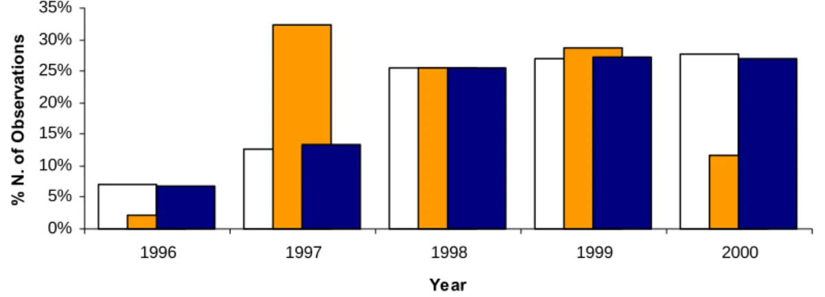
(21) % N. of Observations. 45% 40% 35% 30% 25% 20% 15% 10% 5% 0% A. B. C. D. E. F. G. H. I. K. MNO. Industry Non-Default. Default. Figure 2 – Sample Industry Distribution This figure shows the model sample industry distributions for the firms that defaulted and for the firms that have not defaulted. The industry types considered are: A – Agriculture, Hunting & Forestry; B – Fishing; C – Mining & Quarrying; D – Manufacturing; E – Electricity, Gas & Water Supply; F – Construction; G – Wholesale & Sale Trade; H – Hotels & Restaurants; I – Transport, Storage & Communications; K – Real Estate, Renting & Business Activities; MNO – Education/ Health & Social Work/ Other Personal Services Activities.. % N. of Observations. 35% 30% 25% 20% 15% 10% 5% 0% 1996. 1997. 1998. 1999. 2000. Year Non-Default. Default. Total. Figure 3 – Accounting Statement Yearly Distribution The figure above displays the yearly distribution of the financial statements in the dataset for the default, non-default and total observations.. 7.

(22) % N. of Observations. 20% 18% 16% 14% 12% 10% 8% 6% 4% 2% 0% 1. 2. 3. 4. 5. 6. 7. 10. 15. 20. 30. 40. 50. 60. 70 More. Turnover, Millions of EUR Non-Default. Default. Figure 4 – Size (Turnover) Distribution, Millions of EUR The figure shows the size distribution of the default and non-default observations. Size is measured by the firms’ Turnover, defined as the sum of total sales plus services rendered.. Analysis of industry distribution (Figure 2) suggests high concentration on industries G – Trade and D – Manufacturing, both accounting for about 75% of the whole sample. The industry distributions for both default and non-default observations are very similar. Figure 3 shows that observations are uniformly distributed per year, for the last three periods, with about 3,000 observations per year. For the non-default group of observations, the number of yearly observations rises steadily until the third period, and then remains constant until the last period. For the default group, the number of yearly observations has a great increase in the second period and clearly decreases in the last. Figure 4 shows size distribution and indicates that most of the observations belong to the Small and Medium size Enterprises - SME segment, with annual turnover up to 50 million EUR (according to the NBCA SME classification). The SME segment accounts for about 95% of the whole sample. The distributions of both non-default and default observations are very similar.. 8.

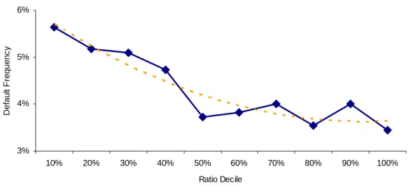
(23) 3. Financial Ratios and Bivariate Analysis. A preliminary step before estimating the scoring model is to conduct a bivariate analysis for each potential explanatory variable, in order to select the most intuitive and powerful ones. In this study, the scoring model considers exclusively financial ratios as explanatory variables. A list of twenty-three ratios representing six different dimensions – Profitability, Liquidity, Leverage, Debt Coverage, Activity and Productivity – is considered. The bivariate analysis relates each of the twenty-three ratios and a default indicator, in order to assess the discriminatory power of each variable. Appendix 1 provides the list of the variables and how they are constructed. Figures 5 – 10 provide a graphical description, for some selected variables, of the relationship between each variable individually and the default frequency. The data is ordered in ascending order by the value of each ratio and, for each decile, the default frequency is calculated (number of defaults divided by the total number of observations in each decile).. Default Frequency. 6%. 5%. 4%. 3%. 2% 10%. 20%. 30%. 40%. 50%. 60%. 70%. 80%. 90%. 100%. Ratio Decile. Figure 5 – Average Default Frequency by Liquidity / Current Liabilities Ratio Decile The figure shows the relationship between the Liquidity / Current Liabilities Ratio and the historical default frequency. Loans are ranked in ascending order, in terms of the value of the ratio. For each decile the average default frequency is calculated.. 9.

(24) Default Frequency. 6%. 5%. 4%. 3% 10%. 20%. 30%. 40%. 50%. 60%. 70%. 80%. 90%. 100%. Ratio Decile. Figure 6 – Average Default Frequency by Current Ratio Decile The figure shows the relationship between the Current Ratio and the historical default frequency. Loans are ranked in ascending order, in terms of the value of the ratio. For each decile the average default frequency is calculated.. Default Frequency. 6%. 5%. 4%. 3%. 2% 10%. 20%. 30%. 40%. 50%. 60%. 70%. 80%. 90%. 100%. Ratio Decile. Figure 7 – Average Default Frequency by Liquidity / Assets Ratio Decile The figure shows the relationship between the Liquidity / Assets Ratio and the historical default frequency. Loans are ranked in ascending order, in terms of the value of the ratio. For each decile the average default frequency is calculated.. 10.

(25) 9%. Default Frequency. 8% 7% 6% 5% 4% 3% 2% 1% 0% 10%. 20%. 30%. 40%. 50%. 60%. 70%. 80%. 90%. 100%. Ratio Decile. Default Frequency. Figure 8 – Average Default Frequency by Debt Service Coverage Ratio Decile The figure shows the relationship between the Debt Service Coverage Ratio and the historical default frequency. Loans are ranked in ascending order, in terms of the value of the ratio. For each decile the average default frequency is calculated.. 13% 12% 11% 10% 9% 8% 7% 6% 5% 4% 3% 2% 1% 0% 10%. 20%. 30%. 40%. 50%. 60%. 70%. 80%. 90%. 100%. Ratio Decile. Figure 9 – Average Default Frequency by Interest Costs / Sales Ratio Decile The figure shows the relationship between the Interest Costs / Sales Ratio and the historical default frequency. Loans are ranked in ascending order, in terms of the value of the ratio. For each decile the average default frequency is calculated.. 11.

(26) 8%. Default Frequency. 7% 6% 5% 4% 3% 2% 10%. 20%. 30%. 40%. 50%. 60%. 70%. 80%. 90%. 100%. Ratio Decile. Figure 10 – Average Default Frequency by Productivity Ratio Decile The figure shows the relationship between the Productivity Ratio and the historical default frequency. Loans are ranked in ascending order, in terms of the value of the ratio. For each decile the average default frequency is calculated.. In order to have a quantitative assessment of the discriminating power of each variable, the Accuracy Ratio is used7. The computed values of the Accuracy Ratios are reported in Appendix 1. The selected variables for the multivariate analysis comply with the following criteria: -. They must have discriminating power, with an Accuracy Ratio higher than 5%;. -. The relationship with the default frequency should be clear and economically intuitive. For example, ratio Current Earnings and Depreciation / Turnover should have a negative relationship with the default frequency, since firms with a high percentage of EBITDA over Turnover should default less frequently; analyzing Figure 11, there seems to be no clear relationship for this dataset;. -. The number of observations lost due to lack of information on any of the components of a given ratio must be insignificant. Not all firms have the same. 7. The Accuracy Ratio can be used as a measure of the discriminating power of a variable, comparing the ability of the variable to correctly classify the default and non-default observations against that of a random variable, unrelated to the default process. Section 4.1.1 provides a more detailed description.. 12.

(27) degree of accuracy on their accounting reports, for example, ratios Bank Debt / Accounts Payable and P&L / L-T Liabilities have a significant amount of missing data for the components Debt to Credit Institutions and Long-Term Liabilities respectively.. Default Frequency. 6%. 5%. 4%. 3% 10%. 20%. 30%. 40%. 50%. 60%. 70%. 80%. 90%. 100%. Ratio Decile. Figure 11 – Average Default Frequency by Current Earnings and Depreciation / Turnover Ratio Decile The figure shows the relationship between the Current Earnings and Depreciation / Turnover Ratio and the historical default frequency. Loans are ranked in ascending order, in terms of the value of the ratio. For each decile the average default frequency is calculated.. At this point, nine variables are eliminated and are not considered on the multivariate analysis. All the remaining variables are standardized in order to avoid scaling issues8.. 8. Standardization consists on subtracting the value of the variable by its average on the sample and dividing the result by its sample standard deviation.. 13.

(28) 4. Scoring Model and Validation. The dependent variable Yit is the binary discrete variable that indicates whether firm i has defaulted (one) or not (zero) in year t. The general representation of the model is:. Yit = f ( β k , X itk−1 ) + eit ,. (1). where X itk−1 represents the values of the k explanatory variables of firm i, one year before the evaluation of the dependent variable. The functional form selected for this study is the Logit model9. Alternative specifications can be considered, such as Probit, Linear Probability Model, or even Genetic Algorithms, although there is no evidence in the literature that any alternative specification can consistently outperform the Logit specification in credit default prediction (Altman, Marco and Varetto, 1994 and Yang et al., 1999). Using both forward and backward procedures, the selected model is the one that complies with the validation criteria and has the higher discriminating power, measured by the Accuracy Ratio.. 4.1. Model Validation. The variables selected on Section 3 are pooled together in order to obtain a model that is at the same time: -. Parsimonious but powerful: high discriminating power with few parameters to estimate;. -. Statistically significant: all variables individually and the model as a whole must be significant, with low correlation between the variables;. 9. Refer to Appendix 3 for a description of the Logit model.. 14.

(29) -. Intuitive: the sign of the estimated parameters should make economic sense and the selected variables should represent the various relevant risk factors.. 4.1.1. Efficiency. A model with high discriminatory power is a model that can clearly distinguish the default and non-default populations. In other words, it is a model that makes consistently “good” predictions relative to few “bad” predictions. For a given cut-off value10, there are two types of “good” and “bad” predictions: Estimated. Observed. Non-Default. •. Non-Default Default. True Miss (Type I Error). Default False Alarm (Type II Error) Hit. The “good” predictions occur if, for a given cut-off point, the model predicts a default and the firm does actually default (Hit), or, if the model predicts a non-default and the firm does not default in the subsequent period (True).. •. The “bad” prediction occurs if, for a given cut-off point, the model predicts a default and the firm does not actually defaults (False-Alarm or Type II Error), or if the model predicts a non-default and the firm actually defaults (Miss or Type I Error).. •. The Hit Ratio (HR) corresponds to the percentage of defaults from the total default population that are correctly predicted by the model, for a given cut-off point.. 10. The cut-off point is the value from which the observations are classified as “good” or “bad”. For example, given a cut-off point of 50%, all observations with an estimated score between 0% and 50% will be classified as “good”, and those between 50% and 100% will be considered “bad”.. 15.

(30) •. The False Alarm Ratio (FAR) is the percentage of False Alarms or incorrect default predictions from the total non-defaulting population, for a given cut-off point.. Several alternatives could have been considered in order to analyze the discriminating power of the estimated models. In this study, both ROC/CAP analysis and Kolmogorov-Smirnov (KS) analysis are performed. Receiver Operating Characteristics (ROC) and Cumulative Accuracy Profiles (CAP) curves are two closely related graphical representations of the discriminatory power of a scoring system. Using the notation from Sobehart and Keenan (2001), the ROC curve is a plot of the HR against the FAR, while the CAP curve is a plot of the HR against the percentage of the sample. For the ROC curve, a perfect model would pass through the point (0,1) since it always makes “good” predictions, and never “bad” predictions (it has FAR = 0% and a HR = 100% for all possible cut-off points). A “naïve” model is not able to distinguish defaulting from non-defaulting firms, thus will do as many “good” as “bad” predictions, though for each cut-off point, the HR will be equal to the FAR. A better model would have a steeper curve, closer to the perfect model, thus a global measure of the discriminant power of the model would be the area under the ROC curve. This can be calculated as11: 1. AUROC = ∫ HR( FAR)d ( FAR),. (2). 0. For the CAP or Lorenz curve, a perfect model would attribute the lowest scores to all the defaulting firms, so if x% of the total population are defaults, then the CAP curve of a perfect model would pass through the point (x,1). A random model would make as many “good” as “bad” predictions, so for the y% lowest scored firms it would have a HR of y%. Then, a global measure of the discriminant power of the model, the Accuracy Ratio (AR), compares the area between the CAP curve of the. 11. Refer to Appendix 2 for a technical description of the AUROC calculation.. 16.

(31) model being tested and the CAP of the random model, against the area between the CAP curve of the perfect model and the CAP curve of the random model. It can be shown that there is a linear relationship between the global measures resulting from the ROC and CAP curves12: AR = 2 ( AUROC − 0.5 ) ,. (3). The KS methodology considers the distance between the distributions of 1 – HR (or Type I Errors) and 1 – FAR (or True predictions) 13. The higher the distance between the two distributions, the better the discriminating power of the model. The KS statistic corresponds to the maximum difference for any cut-off point between the 1 – FAR and 1 – HR distributions.. 4.1.2. Statistical Significance. All estimated regressions are subject to a variety of statistical tests, in order to ensure the quality of the results at several levels: i.. Residual Analysis is performed with the purpose of testing the distributional assumption of the errors of the regression. Although the logistic regression assumes that the errors follow a binomial distribution, for large samples (such as the one in this study), it approximates the normal distribution. The standardized residuals from the logistic regressions should then follow a standard normal distribution14. At this stage, severe outliers are identified and eliminated. These outliers are observations for which the model fits poorly. 12. See, for example, Engelmann, Hayden and Tasche (2003). The Kolmogorov-Smirnov statistic is a non-parametric statistic used to test whether the density function of a variable is the same for two different groups (Conover, 1999). 14 The standardized residuals correspond to the residuals adjusted by their standard errors. This adjustment is made in logistic regression because the error variance is a function of the conditional mean of the dependent variable. 13. 17.

(32) (has an absolute studentized residual15 greater than 2), and that can have a very large influence on the estimates of the model (a large DBeta16). ii.. The significance of each estimated coefficient is tested using the Wald test. This test compares the maximum likelihood value of the estimated coefficient to the estimate of its standard error. This test statistic follows a standard normal distribution under the hypothesis that the estimated coefficient is null. For the three models, all of the estimated coefficients are significant at a 90% significance level.. iii.. In order to test the overall significance of each estimated model, the HosmerLemeshow (H-L) test is used. This goodness-of-fit test compares the predicted outcomes of the logistic regression with the observed data by grouping observations into risk deciles.. iv.. After selecting the best linear model, the assumption of linearity between each variable and the logit of the dependent variable is checked. This is performed in four stages: 1-. The Box-Tidwell test (Box-Tidwell, 1962) is performed on all. continuous variables, in order to confirm the linearity assumption; 2-. For all variables that failed the linearity test in the previous step, a plot. of the relationship between the covariate and the logit is presented, providing evidence on the type of non-linear relationship; 3-. For all continuous variables with significant non-linear relationships. with the logit, the fractional polynomial methodology is implemented (Royston and Altman, 1994) in order to adequately capture the true relationship between the variables; 4v.. Check whether the selected transformation makes economic sense.. The last assumption to be checked is the independence between the explanatory variables. If multicolinearity is present, the estimated coefficients. 15. The studentized residual corresponds to the square root of the change in the -2 Log Likelihood of the model attributable to deleting the case from the analysis. It follows an asymptotical normal distribution and extreme values indicate a poor fit. 16 DBeta is an indicator of the standardized change in the regression estimates obtained by deleting an individual observation.. 18.

(33) will be unbiased but their estimated standard errors will tend to be large. In order to test for the presence of high multicolinearity, a linear regression model using the same dependent and independent variables is estimated, and the tolerance statistic is calculated for each independent variable17. If any of the tolerance statistics are below 0.20 then it is assumed that we are in the presence of high multicolinearity, and the estimated regression is discarded.. 4.1.3. Economic Intuition. All estimated coefficients follow economic intuition in the sense that the sign of the coefficients indicates the expected relationship between the selected variable and the default frequency. For example, if for a given model the estimated coefficient for variable Productivity Ratio is +0.123, this means that the higher the Personnel Costs relative to the Turnover, the higher the estimated credit score of the firm. In other words, firms with lower labor productivity have higher credit risk. For the non-linear relationships it is best to observe graphically the estimated relationship between the independent variable and the logit of the dependent. As for the linear case, this relationship should be monotonic, either always positive or negative. The difference is that the intensity of this relationship is not constant, it depends on the level of the independent variable. During the model estimation two hypotheses are tested: 1. Whether a system of unrelated equations, by industry group yields better results than a single-equation model for all industries; 2. Whether a model where the observations are weighted in order to increase the proportion of defaults to non-defaults in the estimation sample, performs better than a model with unweighted observations.. 17. The tolerance statistic corresponds to the variance in each independent variable that is not explained by all of the other independent variables.. 19.

(34) 4.2. Model A – Multiple Industry Equations Model. In order to test the hypothesis that a system of unrelated equations by industry group yields better results than a single-equation model for all industries, the dataset is broken into two sub-samples: the first one for Manufacturing & Primary Activity firms, with 5,046 observations of which 227 are defaults; and the second for Trade & Services firms, with 5,954 observations and 248 defaults. If the nature of these economic activities has a significant and consistent impact on the structure of the accounting reports, then it is likely that a model accommodating different variables for the different industry sectors performs better than a model which forces the same variables and parameters to all firms across industries18. The model is: exp ( µˆ i ) Yˆi = , 1 + exp ( µˆ i ). (4). for the two-equation model, ⎧⎪ X ia ' βˆ a b b ⎪⎩ X i ' βˆ. µˆ i = ⎨. if i belongs to industry a if i belongs to industry b. ,. (5). for the single-equation model,. µˆ i = X i ' βˆ. ∀i,. (6). For the final model, the selected variables and estimated coefficients are presented in the table below19:. 18. Model performance is measured by the ability to discriminate between default and non-default populations, which can be summarized by the Accuracy Ratio. 19 Refer to Appendix 4 for full estimation results.. 20.

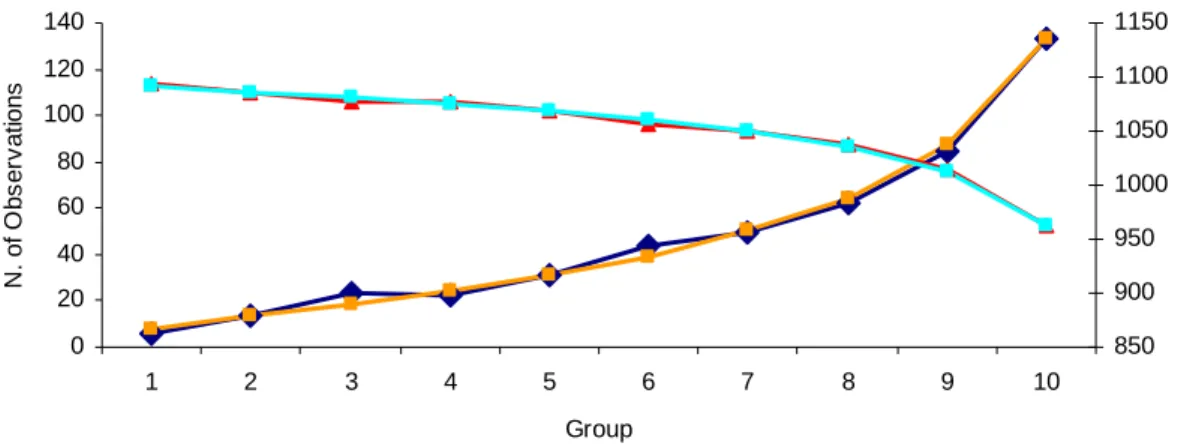
(35) Industry a. Industry b. Wald Test Wald Test Variable Variable βˆ βˆ P-Value P-Value Liquidity / CurLiabilities -0.381 0.003 Current Ratio -0.212 0.005 Debt Service Coverage -0.225 0.021 Liquidity / Assets -0.160 0.063 Interest Costs / Sales_1 2.011 0.002 Debt Service Coverage -0.184 0.041 Interest Costs / Sales_2 -0.009 0.000 Interest Costs / Sales_1 1.792 0.000 Productivity Ratio 0.200 0.028 Interest Costs / Sales_2 -0.009 0.038 Constant -3.259 0.000 Constant -3.426 0.000 5,044 5,951 Number of Observations Number of Observations 1,682 1,913 -2 LogLikelihood -2 LogLikelihood 0.415 0.615 H-L Test P-Value H-L Test P-Value Table 1 – Estimated Model Variables and Parameters, Model (A) The table above presents the estimation results for the two industry equation model. Industry a represents Manufacturing & Primary Activity firms, and Industry b Trade & Services firms. The sign of the estimated parameters for both regressions is in accordance with economic intuition. The significance of each parameter is demonstrated by the low p-values for the Wald test, while the overall significance of each regression is verified by the high p-values for the Hosmer-Lemeshow test.. The Hosmer-Lemeshow test is a measure of the overall significance of the logistic regression. Through the analysis of Figure 12 we can conclude that the. N. of Observations. estimated logistic regressions significantly fit the observed data.. 140. 1150. 120. 1100. 100. 1050. 80. 1000. 60. 950. 40. 900. 20 0. 850 1. 2. 3. 4. 5. 6. 7. 8. 9. 10. Group Observed Defaults. Expected Defaults. Observed Non-Defaults. Expected Non-Defaults. Figure 12 – Model A: Hosmer-Lemeshow Test This figure presents the comparison between the observed and expected number of default and nondefault observations for each of the 10 groups comprised in the Hosmer-Lemeshow test. The number of the default observations is represented on the left y axis, while the number of non-default observations is represented on the right y axis.. 21.

(36) 4.3. Model B – Standard Model. In order to test our two hypotheses both the Two-Equation Model and the Weighted Sample Model will be evaluated against the standard setting of a single equation across all industries, using an unweighted sample. Table 2 summarizes the final results under this standard setting and Figure 13 provides a graphical description of the overall significance of the estimated model. Wald Test P-Value Current Ratio -0.171 0.001 Liquidity / Assets -0.211 0.002 Debt Service Coverage -0.231 0.001 Interest Costs / Sales_1 1.843 0.007 Interest Costs / Sales_2 -0.009 0.000 Productivity Ratio 0.124 0.003 Constant -3.250 0.000 10,995 Number of Observations 3,600 -2 LogLikelihood 0.973 H-L Test P-Value Table 2 – Estimated Model Variables and Parameters, Model (B) This table displays the estimation results for the single-equation model. The sign of the estimated parameters agrees with economic intuition. The significance of each parameter is demonstrated by the low p-values for the Wald test, while the overall significance of the regression is verified by the high pvalues for the Hosmer-Lemeshow test.. βˆ. Variable. 22.

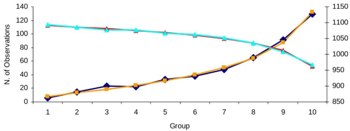
(37) N. of Observations. 140. 1150. 120. 1100. 100. 1050. 80. 1000. 60. 950. 40. 900. 20 0. 850 1. 2. 3. 4. 5. 6. 7. 8. 9. 10. Group Observed Defaults. Expected Defaults. Expected Non-Defaults. Observed Non-Defaults. Figure 13 – Model B: Hosmer-Lemeshow Test This figure presents the comparison between the observed and expected number of default and nondefault observations for each of the 10 groups comprised in the Hosmer-Lemeshow test. The number of the default observations is represented on the left y axis, while the number of non-default observations is represented on the right y axis.. 4.4. Model C – Weighted Sample Model. The proportion of the number of defaults (450) to the total number of observations in the sample (11,000) is artificially high. The real average annual default frequency of the bank’s portfolio and the Portuguese economy is significantly lower than the 4.32% suggested by our sample for the corporate sector. However, in order to be able to correctly identify the risk profiles of “good” and “bad” firms, a significant number of observations for each population is required. For example, keeping the total number of observations constant, if the correct default rate is about 1%, extracting a random sample in accordance to this ratio would result in a proportion of 110 default observations to 11,000 observations. A consequence of having an artificially high proportion of default observations is that the estimated scores cannot be directly interpreted as real probabilities of default. Therefore, these results have to be calibrated in order to obtain default probabilities estimates. A further way to increase the proportion of the number of default observations is to attribute different weights to the default and non-default observations. The 23.

(38) weightening of observations could potentially have two types of positive impact in the analysis: 1. As mentioned above, a more balanced sample, with closer proportion of default to non-default observations, could help the Logit regression to better discriminate between both populations; 2. The higher proportion of default observations results in higher estimated scores. As a consequence, the scores in the weighed model are more evenly spread throughout the ]0,1[ interval (see Figure 14). If, in turn, these scores are used to group the observations into classes, then it could be easier to identify coherent classes with the weighed model scores. Thus, even if weightening the observations does not yield a superior model in terms of discriminating power,. Observation. it might still be helpful later in the analysis, when building the rating classes.. 0%. 10%. 20%. 30%. 40%. 50%. 60%. 70%. 80%. 90%. 100%. Score Unw eighted Model Score. Weighted Model Score. Figure 14 – Weighted vs. Unweighted Score The figure presents the estimated scores for each observation in the development sample using both weighted and unweighted models.. The weighted model estimated considers a proportion of one default observation for two non-default observations. The weighed sample consists of 1,420 observations, of which 470 are defaults and the remaining 950 are non-default. 24.

(39) observations20. The optimized model selects the same variables as the unweighted model though with different estimated coefficients. Wald Test P-Value Current Ratio -0.197 0.003 Liquidity / Assets -0.223 0.006 Debt Service Coverage -0.203 0.013 Interest Costs / Sales_1 1.879 0.050 Interest Costs / Sales_2 -0.009 0.000 Productivity Ratio 0.123 0.023 Constant -0.841 0.000 1,420 Number of Observations 1,608 -2 LogLikelihood 0.465 H-L Test P-Value Table 3 – Estimated Model Variables and Parameters, Model (C) This table shows the estimation results for the weighted sample model. The selected variables are the same as for the unweighted model (B). All estimated parameters are significant at a 5% level and the suggested relationship with the dependent variable concurs with economic intuition. The high p-values for the Hosmer-Lemeshow test attest the overall significance of the regression.. βˆ. N. of Observations. Variable. 100 90 80 70 60 50 40 30 20 10 0. 160 140 120 100 80 60 40 20 0 1. 2. 3. 4. 5. 6. 7. 8. 9. 10. Group Observed Defaults. Expected Defaults. Observed Non-Defaults. Expected Non-Defaults. Figure 15 – Model C: Hosmer-Lemeshow Test This figure presents the comparison between the observed and expected number of default and nondefault observations for each of the 10 groups comprised in the Hosmer-Lemeshow test. The number of the default observations is represented on the left y axis, while the number of non-default observations is represented on the right y axis.. 20. Other proportions yield very similar results (namely the one default for one non-default and one default for three non-defaults proportions).. 25.

(40) The following section analyses the estimation results in more detail and compares the different approaches in terms of efficiency.. 4.5. Analysis of the Results. In Appendix 4, the final results of the estimations are presented for all three models: the two-equation model (Model A), the unweighted single-equation model (Model B) and the weighted single-equation model (Model C). The first step to obtain each model is to find the best linear combination through backward and forward selection procedures. The estimation equation that complies with both economic intuition and positive statistical diagnosis (described in steps i. to iii. of section 4.1.2), and had the higher discriminating power is considered the optimal linear model. The second step is to check for non-linear relationships between the independent variables and the logit of the dependent. Results indicate that for all four selected linear regressions, there is a clear non-linear relationship between variable Interest Costs / Sales and the logit of the dependent variable. In order to account for. this fact, the procedure described in step iv. of section 4.1.2 is implemented. The resulting non-linear relationship for the four regressions is illustrated in Figure 16. In order to depict graphically the relationship between the covariate and the binary dependent variable, a Locally Weighted Scatterplot Smoothing, or Lowess (Cleveland 1979), was created. In addition, the quality of the fit of this relationship for the three estimated models can be accessed by comparing the multivariate adjustment for each model with the lowess curve. For all three models, the quality of the adjustment is high but deteriorates for very high values of the explanatory variable.. 26.

(41) 0 0. 1. 2. 3. 4. 5. 6. -1. Logit. -2. -3. -4. -5. -6 Var 20 Low ess Var 20. Multivariate Model A. Multivariate Model B. Multivariate Model C. Figure 16 – Smoothed Lowess and Fractional Polynomial Adjustment for the Interest Costs / Sales Ratio The figure compares the plot of the bivariate smoothed Lowess logit of the variable Interest Costs / Sales with the multivariate fractional polynomial adjustment for models A – Multiple Industry Equations Model, B – Standard Model and C – Weighted Sample Model.. After the optimal non-linear regressions are selected, a final test for multicolinearity is implemented. Only the Trade & Services regression of the TwoEquation Model presented signs of severe multicolinearity. Since there is no practical method to correct this problem, the model is discarded and the second best model suggested by the fractional polynomial procedure is selected. This alternative specification does not suffer from multicolinearity, as it can be observed in the results presented in Appendix 421. In short, the modeling procedure consisted on selecting the best discriminating regression from a pool of possible solutions that simultaneously complied with economic and statistical criteria. In terms of efficiency, all three models have a small number of selected variables: model A has five variables for each equation, while models B and C have six variables each. Analyzing Figures 17 and 18, we can conclude that all three models have significant discriminating power and have similar performances. Results. 21. In order to ensure stability of the final results, the whole modeling procedure is repeated with several random sub-samples of the main dataset. Across all sub-samples the variables selected for each model are the same, the values of the estimated coefficients are stable, and the estimated AR’s are similar.. 27.

(42) for Altman’s Z’-Score Model for Private Firms (Altman, 2000) are also reported as a benchmark (Model D). Figure 17 displays the Receiver Operating Characteristics (ROC) curves. The ROC curve provides for each possible cut-off value the proportion of observations incorrectly classified as default by the model against the proportion correctly classified as default. The three suggested models have similar ROC curves, clearly above the Random Model and Z’-Score Model curves.. 100% 90% 80% 70%. HR. 60% 50% 40% 30% 20% 10% 0% 0%. 10%. 20%. 30%. 40%. 50%. 60%. 70%. 80%. 90%. 100%. FAR Model A. Model B. Model C. Model D. Random Model. Figure 17 – Receiver Operating Characteristics Curves The figure above displays the Receiver Operating Characteristics curves for the three estimated models (A – Multiple Industry Equations Model, B – Standard Model and C – Weighted Sample Model) and for the Z’-Score Model for Private Firms (Altman, 2000). The ROC curve provides for each possible cut-off value the proportion of observations incorrectly classified as default by the model, the False Alarm Ratio (FAR), against the proportion correctly classified as default, the Hit Ratio (HR).. Figure 18 displays the Cumulative Accuracy Profiles (CAP) curves. The CAP curve provides, for a given proportion of observations with the highest estimated scores, the proportion of correctly classified default observations. As with the ROC analysis, the curves for the three selected models are similar and clearly above the Random Model and Z’-Score Model curves.. 28.

(43) 100% 90% 80% 70%. HR. 60% 50% 40% 30% 20% 10% 0% 0%. 10%. 20%. 30%. 40%. 50%. 60%. 70%. 80%. 90%. 100%. % of Sam ple Perfect Model. Model A. Model B. Model C. Model D. Radom Model. Figure 18 – Cumulative Accuracy Profiles Curves This figure displays the Cumulative Accuracy Profiles curves for the three estimated models (A – Multiple Industry Equations Model, B – Standard Model and C – Weighted Sample Model) and for the Z’-Score model (Model D). The CAP curve provides, for a given proportion of observations with the highest estimated scores, the proportion of correctly classified default observations (the Hit Ratio, HR).. Figures 23-28 in Appendix 5 provide both the Kolmogorov-Smirnov (KS) analysis and Error Type curves. The KS analysis consists on evaluating for each possible cut-off point the distance between the Type I Error curve and the True Prediction curve. The higher the distance between the curves, the better the discriminating power of the model. The Error Type curves display for each cut-off point the percentages of Type I (incorrectly classifying an observation as non-default) and Type II (incorrectly classifying an observation as default) errors for each model.. 29.

(44) Table 4 summarizes the results for both ROC/CAP analysis and KS analysis, under both the estimation and testing samples. All three measures of discriminating power, under both samples, indicate similar and positive values for the three models estimated, clearly above the Z’-Score model.. Model. Main Sample AUROC. σAUROC. Out-of-Sample. AR. KS. AUROC. σAUROC. AR. 1.15% 43.75% 32.15% 73.04% 7.53% 46.07% 1.15% 43.77% 32.97% 75.29% 6.55% 50.59% 1.15% 43.74% 32.94% 74.15% 6.88% 48.29% 1.25% 25.07% 19.77% 61.11% 6.87% 22.22% Table 4 – AUROC, AR and KS Statistics This table reports the Area Under the ROC curves, Accuracy Ratios and Kolmogorov-Smirnov statistics estimated for the three suggested models (A – Multiple Industry Equations Model, B – Standard Model and C – Weighted Sample Model) and for the Z’-Score model (Model D), under both the estimation and testing samples. A B C D. 71.88% 71.88% 71.87% 62.53%. A more rigorous comparison of the discriminating power of the models can be obtained through a statistical test presented in DeLong et al. (1988) for the difference between the estimated AUROC’s of the different models22. Table 5 presents the results of applying this test to the differences between all models for both samples.. Test. Main Sample θi - θj. σ (θi - θj). Out-of-Sample P-Value. θi - θj. σ (θi - θj). P-Value. -0.0089% 0.2225% 96.83% -2.2571% 2.8844% 43.39% 0.0053% 0.2372% 98.23% -1.1086% 2.7449% 68.63% 9.3425% 1.7807% 0.00% 11.9256% 7.7745% 12.50% 0.0141% 0.0476% 76.68% 1.1485% 0.5115% 2.47% 9.3514% 1.7788% 0.00% 14.1827% 6.7577% 3.58% 9.3372% 1.7751% 0.00% 13.0342% 7.0051% 6.28% Table 5 – Testing the Differences between AUROC’s The table above provides the results of a statistical test for comparing the estimated AUROC curves between the different models. Model A is the Multiple Industry Equations model, Model B the Standard Model, Model C the Weighted Sample and Model D the Z’-Score model. A-B A-C A-D B-C B-D C-D. The results indicate that for both samples, Models A, B and C have similar discriminating power, and all three perform significantly better that the Z’-Score model.. 22. For a description of the test consult Appendix 2.. 30.

(45) Regarding our first hypothesis that a setting with multiple equations could yield better results, both in-sample and out-of-sample results suggest there is no improvement from the standard approach. The estimated Accuracy Ratio for the twoequation model is 43.75%, which is slightly worse than the Accuracy Ratio of the single-equation model, 43.77%. The out-of-sample results confirm this tendency, the AR of the two-equation model is 46.07%, against 50.59% of the single-equation model, according to the test results presented in Table 5 none of these differences is statistically significant. Since the two-equation model involves more parameters to estimate and is not able to better discriminate to a significant extent the default and non-default populations of the dataset, the single-equation specification is considered superior in terms of scoring methodology for this dataset. Regarding the hypothesis that balancing the default and non-default populations could help the logistic regression to better discriminate them, again both in-sample and out-of-sample results do not provide positive evidence. The estimated Accuracy Ratio for the weighed model is 43.74%, marginally worse than the 43.77% of the unweighted model. Again, the out-of-sample results confirm that the weighted model does not have a higher discriminating power (AR of 48.29%) than the unweighted model (AR of 50.59%). As reference, the private-firm model developed by Moody’s to the Portuguese market has an in-sample AR of 61.1% (unfortunately no out-of-sample AR is reported)23. The selected variables are: Equity / Total Accounts Payable, Bank Debt / Total Liabilities, Net P&L / Assets, (Ordinary P&L+ Depreciation)/ Interest and similar Expenses, (Ordinary P&L + Depreciation + Provisions) / Total Liabilities, Current Assets / Accounts Payable (due within 1 year) and Interest and similar Expenses / Turnover. The sample data comprised financial statements of 18,137. unique firms, of which 416 had defaulted (using the “90 days past due” definition), with a time span from 1993 to 2000. Hayden (2003) reports an in-sample AR of 50.3% and an out-of-sample AR of 48.8% for a logistic regression model applied to the Austrian market, with the “90 days past due” default definition. The variables selected are Equity / Assets, Bank Debt / Assets, Current Liabilities / Assets, Accounts. 23. See Murphy et al. (2002). 31.

(46) Payable / Mat. Costs, Ordinary Business Income / Assets and Legal Form. The. sample data included 16,797 observations, of which 1,604 were defaults, for a time period ranging from 1992 to 1999. Due to differences in the dataset, such as different levels of data quality or the ratio of default to non-default observations, the reported AR’s for both studies presented above cannot be directly comparable to the AR’s reported in our study. Despite this fact, they can still be regarded as references that attest the quality of the model presented in terms of discriminatory power. The following chapter discusses possible applications of the scoring model presented. We start by discussing the creation of a quantitative rating system, followed by the estimation of probabilities of default and rating transition matrixes. Finally the capital requirements for a simulated portfolio are calculated under both the NBCA and current regulations.. 32.