726 Brazilian Journal of Physics, vol. 37, no. 2C, June, 2007
Obtaining Femtoscopy Results in Models with Resonances
Adam Kisiel
Faculty of Physics, Warsaw University of Technology, ul. Koszykowa 75, 00-662 Warsaw, Poland
Received on 23 November, 2006; revised version received on 16 March, 2007
We present femtoscopic results from models in which the resonance contribution is taken into account. The Therminator program, which implements a single freeze-out model and takes into account propagation and decay of all known resonances, was used. We test methods of determining the femtoscopic size of the system, or the “HBT radii”. We show that the best one is the two-particle method combined with the exact calculation of the two-pion wave function including the wave-function symmetrization and Coulomb effects. We compare it to other methods and comment on their validity and applicability.
Keywords: Femtoscopy; Resonance propagation; HBT radii
I. FEMTOSCOPIC DEFINITIONS
The femtoscopy measurements have been extensively used to study the heavy-ion collisions. For recent review of theo-retical and experimental results please see [1]. Femtoscopic correlation function is normally constructed as:
C(~q, ~K) =P C 2(~q, ~K)
P20(~q, ~K) (1) whereP2C is the probability to observe two femtoscopically correlated particles at relative momentum~q.P20is such prob-ability where the correlation between particles does not have the femtoscopic component. ~Kis the average momentum of the pair. In heavy-ion experiments the PC
2 is usually con-structed from pairs coming from the same event;P0
2from pairs where each particle comes from different event, but the events are as close to each other in global characteristics as possible. In theoretical models one should, in principle, generate par-ticles in such a way that they are already correlated due to their mutual and many-particle interactions. That is however usually computationally not possible. One then makes an as-sumption that the interaction between particles can be sep-arated from their generation and we write the most general form of the correlation function that can be used by models:
C(~q, ~K) =
R
S(r∗,~q, ~K)|Ψ(~q,r∗)|2d4r∗
R
S(r∗,~q, ~K)d4r∗ (2)
wherer∗is the pair separation in the pair rest frame (PRF) and S(r∗,~q, ~K)is the pair separation distribution constructed as: S(r∗,~q, ~K) =
Z
S1(x1,~p1)S2(r∗−x2,~p2)δ(r∗−x1+x2)d4x1d4x2 (3) andS(x,~p)is the single-particle emission function provided by the model. For identical particles S1≡S2 and S(r∗) is symmetric by definition, for non-identical particles S(r∗) is usually asymmetric. In this work we only consider identical particles, more specifically charged pions. If one takes into account the proper symmetrization of the wave function only:
¯
¯Ψ(~q,r∗)Q ¯ ¯
2
=1+cos(~q~r∗) (4)
one obtains a quantum-statistics only correlation functionCQ which has a simple form and is useful in model studies. One can also consider Coulomb interaction:
¯
¯Ψ(~q,r∗)QC ¯ ¯
2 = |
√ AC √
2 [exp(−i
~k∗~r∗)F(−iη,1,iξ+) (5)
+ exp(i~k∗~r∗)F(−iη,1,iξ−)]|2 (6) wherek∗is half of pair relative momentum in PRF,AC is the Gamow factor, F is the confluent hypergeometric function, η=1/k∗ac,acis the pair Bohr radius andξ±=k∗r∗±~k∗~r∗. Then one obtains the full correlation function that can be com-pared to data.
It is possible to use Eq. 2 to get the model correlation func-tion. However it is often difficult to perform the complete in-tegration, so various approximations are used, which will be presented in the next sections. Another possibility is to per-form the integral numerically. One needs to generate particles according to the single-particle emission function. Then one combines the particles into pairs and creates two histograms -in one of them the squared wave-function of the pair is stored, in the other: unity for each pair. The result of the division of the two histograms is the average pair wave function in each bin, which is the correlation function per Eq. (2).
II. OBTAINING HBT RADII
Femtoscopic analysis provides information about the size of the system in terms of the “HBT radii”. It is also possi-ble to obtain information about the separation distribution in a model independent way using the “imaging” technique [2, 3]. The size of the system can be determined separately in three directions: “out” - along the pair momentum, “long” - along the beam axis and “side” - perpendicular to the other two. All analysis are performed in LCMS system, which is defined as the one in which pair momentum along the beam axis van-ishes. The radii are obtained under the following assumptions. The emission function is static (does not depend on particle’s momentum) and is a 3d sphere with gaussian density profile:
S(r)≈exp
Ã
−rout2 4R2out+
−r2 side 4R2side+
−rlong2 4R2long
!
Adam Kisiel 727
The correlation function is then:
C(~q) =1+λexp(−R2outq2out−R2sideq2side−R2longq2long) (8) and can be easily fit to the experimental one to obtain the “HBT radii”Rout,RsideandRlong.
Two other methods of obtaining the radii have been tested. They involve more assumptions, but are simpler to perform analytically. We will test their validity.
The distribution in Eq. (7) is a convolution of two single-particle distributions (see Eq. (3)). It can approximated by the square of them:
S(r)≈S(~x,~p)2 (9) where~pis substituted for ~K. This is rigorously true only if S(x,p)is a static Gaussian. For any realistic Sit is only an approximation, the validity of which is under study. Using Eq. (9) and Eq. (4) one can write the following approximate formula for the correlation function, known as the “Wigner formalism”:
C(~q) =
¯ ¯ R
S(~x,~p)ei~q~xd3x¯ ¯
2
|R
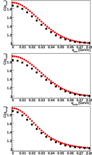
S(~x,~p)d3x|2 (10) This function can again be fit by Eq. (8) to obtain the “HBT radii”. The advantage of this procedure is that it can be per-formed analytically using only the single-particle emission function. An example of the correlation function calculated in this way is shown in Fig. 1, together with the reference function from the two-particle method.
An even simpler procedure is to analyze the emission func-tion Sdirectly. One can either obtain its Gaussian width or calculate the relevant RMS’es. One can do it to single particle emission functionS(~x), which is easier to do, but involves ad-ditional approximation, or to the two particle emission func-tion S(~r). For the exact formulas used in the calculation of RMS’es ofS(~x)please consult [4]. Again these methods will give results identical to the previous ones only if the emission functions are Gaussian. The validity of the approximations was tested, the results are discussed in the next paragraph.
III. METHOD OF TESTING
We test and compare various methods to obtain the “HBT radii”. We treat the two-particle method with the wave-function calculation as the reference, or the method which most closely resembles the experimental one, to which it should be compared.
The input data were the events generated with the THER-MINATOR [5] which takes into account all the resonances from the PDG [6]. It uses the Blast-wave-like model with parameters fit to RHIC central data and a freeze-out hyper-surface with negative slope inρ−t plane (outside-in freeze-out). The two-particle method, described in detail in [7], was used to get the reference radii. The correlation functions ac-cording to (10) were calculated using the same events and a Monte-Carlo integration on a 3-dimensional mesh in~qspace.
[GeV/c] out q
0 0.01 0.02 0.03 0.04 0.05 0.06 0.07 0.08
)
out
C(q
1 1.2 1.4 1.6 1.8
[GeV/c] side q
0 0.01 0.02 0.03 0.04 0.05 0.06 0.07 0.08
)
side
C(q
1 1.2 1.4 1.6 1.8
[GeV/c] long q
0 0.01 0.02 0.03 0.04 0.05 0.06 0.07 0.08
)
long
C(q
1 1.2 1.4 1.6 1.8
FIG. 1: Examples of projections of 3D correlation functions. From top to bottom:C(qout),C(qside)andC(qlong), with other components
ofqintegrated over the range of 10MeV. Black squares are the cor-relation function from the reference two-particle method. Red circles are the correlation function calculated using the Wigner formalism.
The corresponding variances were also calculated, according to formulas given for HBT radii in [4].
728 Brazilian Journal of Physics, vol. 37, no. 2C, June, 2007
t<50 t<100 t<200 t<500 t<1000
t<50 t<100 t<200 t<500 t<1000
[fm]
out
r
4 5 6 7 8 9
t<50 t<100 t<200 t<500 t<1000
t<50 t<100 t<200 t<500 t<1000
[fm]
side
r
4 5 6 7 8 9
t<50 t<100 t<200 t<500 t<1000
t<50 t<100 t<200 t<500 t<1000
[fm]
long
r
4 5 6 7 8 9
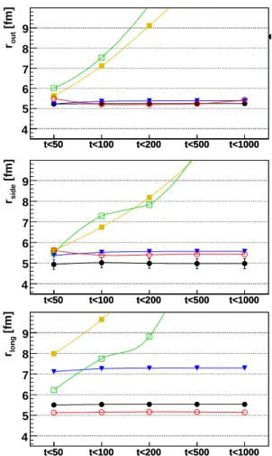
FIG. 2: “HBT radii” as a function of the maximum emission time cut-off. From top to bottom: rout,rsideandrlong. Black filled
circles are the reference twoparticle method. Filled yellow squares -RMS ofS(~r), blue triangles -σof Gaussian fit toS(~r), open green squares - RMS ofS(~x), open red circles: “HBT radii” from the fit to single particle (calculated using the Wigner formalism) correlation function.
IV. RESULTS AND DISCUSSION
The main result of this study is shown in Fig. 2. Several conclusions can be drawn. First, any measure based on the RMS ofS(~x)orS(~r)is not a good approximation of the “HBT radii”. Including strongly decaying resonances makes them go to very large values. It is to be expected as the particles
which decay later, travel some distance before their decay, cre-ating long-range tail in the distributions, to which RMS’es are extremely sensitive. This sensitivity to tails is not present in the radii obtained from the correlation function, and therefore is the weakness of the RMS method.
The next method is the GaussianσofS(~r). It has the de-sired stability versus the time cut-off. However it still can differ from the reference method by up to 30%. Moreover the fitted radius is dependent on the fit range taken. Also this method does not give any reasonable estimate of theλvalue. Therefore it can be used only as a crude estimate of the fem-toscopic radii.
The last method compared is the fit to the correlation func-tion calculated using the Wigner formalism (10). It is stable versus the time cut-off. It shows very good agreement with the reference method for the “out” radius, but the other two can differ up to 10%. It does not permit to calculate the cor-relation function in an arbitrary reference frame, as the two-particle method does. The Coulomb interaction cannot be in-troduced at all, as it can be done only for a pair of particles. A direct comparison of the correlation functions calculated in this way to the reference is shown in Fig. 1. The widths of the functions are comparable, which is also reflected in the radii. However the two-particle function shows lower intercept pa-rameter. In other words theλis overestimated in the Wigner method. The reason is the following. Particles at largerare effectively uncorrelated, and thus lower theλ. So for single-particle emission function we have:
λ= Ns Nl+Ns
= 1−Nl Nl+Ns
(11)
whereNl is the number of particles at large randNs are the particles at smallr(in the source). But a pair is uncorrelated even if only one particle in it is from larger, thereforeλis:
λ= N
2 s (Nl+Ns)2
=1−N 2
l −2NlNs (Nl+Ns)2
(12)
which is smaller than (11) and is the correct value. Therefore the Wigner method can be used when the accuracy of 10% in the radii is acceptable. Also it cannot be used in more ad-vances studies, for example in the direct comparisons of the correlation functions between theory and experiment.
[1] M. A. Lisa, S. Pratt, R. Soltz, and U. Wiedemann, Ann. Rev. Nucl. Part. Sci.55, 357 (2005) [arXiv:nucl-ex/0505014]. [2] D. A. Brown and P. Danielewicz, Phys. Lett. B398, 252 (1997)
[arXiv:nucl-th/9701010].
[3] D. A. Brown, A. Enokizono, M. Heffner, R. Soltz, P. Danielewicz, and S. Pratt, Phys. Rev. C72, 054902 (2005) [arXiv:nucl-th/0507015].
[4] F. Retiere and M. A. Lisa, Phys. Rev. C 70, 044907 (2004)
[arXiv:nucl-th/0312024].
[5] A. Kisiel, T. Taluc, W. Broniowski, and W. Florkowski, Comput. Phys. Commun.174, 669 (2006) [arXiv:nucl-th/0504047]. [6] S. Eidelman, et al., Phys. Lett. B592, 1 (2004)