Topics on Hydrodynamic Model of Nucleus-Nucleus Collisions
Y. Hama
1, T. Kodama
2, and O. Socolowski Jr.
11
Instituto de F´ısica, Universidade de S˜ao Paulo, C.P. 66318, 05315-970 S˜ao Paulo-SP, Brazil
2
Instituto de F´ısica, Universidade Federal do Rio de Janeiro, C.P. 68528, 21945-970 Rio de Janeiro-RJ , Brazil
Received on 15 November, 2004
A survey is given on the applications of hydrodynamic model of nucleus-nucleus collisons, focusing especially on i) the resolution of hydrodynamic equations for arbitrary configurations, by using the smoothed-particle hydrodynamic approach; ii) effects of the event-by-event fluctuation of the initial conditions on the observables; iii) decoupling criteria; iv) analytical solutions; and others.
1
Introduction
Hydrodynamic Model has been proposed by Landau [1] in 1953 as an improvement over the Fermi statistical model [2] for the multiple particle production phenomena in high-energy nuclear collisions. At that time, these phenomena were observed in cosmic rays. Although the Fermi model offered an ingenious insight into the mechanism of the high-energy nuclear collision processes and gave a prediction for the energy dependence of the multiplicity, which was veri-fied by the data, it was known that it had troubles in repro-ducing particle spectra and relative abundance ofKoverπ. This was because, in this model, particles were assumed to be emitted directly from the hot and dense, thermally equi-librated matter formed in high-energy nuclear collisions, which was supposed to be at rest, so that the model predicted isotropic momentum distribution which did not agree with the observed spectra. Furthermore, because of high tem-perature (T >> mK) reached in the process, multiplicity ratio depended only on the isotopic-spin statistical weights, namelyK/π= 4/3. This conclusion of the model was also not in agreement with data.
These problems were solved naturally by letting the hot and dense matter expand before particle emission takes place, reducing thus heavy-particle multiplicities, because of the Boltzmann factor, and giving at the same time alon-gated momentum spectra, due to a violent longitudinal ex-pansion caused by a large pressure gradient in the beam di-rection. A nice feature of this model is that, since the tropy is conserved in the ideal case Landau studied, the en-ergy dependence of the total particle multiplicity predicted by the Fermi model, and verified experimentally, is pre-served.
When accelerator data on multiparticle production be-gan to appear, first inppcollisions at CERN ISR, and later in pp¯ collisions at SppS¯ collider, Carruthers [3] revived thisHeretical Modelin 1974, showing that several aspects of those phenomena may be well understood within Hy-drodynamic Model. When laboratory study of high-energy heavy-nucleus collisions started, Hydrodynamic Model be-came one of the essential tools for these investigations.
According to Hydrodynamic Model, the description of high-energy nuclear collisions goes as follows. At the be-ginning, two Lorentz contracted (in the c.m. frame) nuclei collide and it is assumed that, after a complex process in-volving microscopic collisions of nuclear constituents, a hot and dense matter is formed, which would be in local thermal equilibrium. The description of this initial thermalization process is out of the scope of hydrodynamics. In hydrody-namics, we simply assume that the local thermal equilibrium is attained and these states of matter are specified by some appropriateinitial conditions(IC) in terms of distributions of fluid velocity and thermodynamical quantities for a given time-like parameter. Then, it follows ahydrodynamical ex-pansion, described by the conservation equations of energy-momentum, baryon number and other conserved numbers, such as strangeness, isotopic spin, etc.
∂νTµν = 0 , (1)
∂µ(nBuµ) = 0 , (2)
∂µ(nSuµ) = 0 , (3)
· · · ,
where
Tµν = (ε+p)uµuν−pgµν (4) is the energy-momentum tensor, nB,nS,ε,pare, respec-tively, the baryon number density, the strangeness density, the energy density and the pressure, all of them given in the proper frame of reference of the fluid element, and uµ is the four-velocity of the fluid. Moreover, we have to specify someequations of state(EoS), which depend on the nature of the hot matter produced.
As the expansion proceedes, the fluid becomes cooler and cooler and more rarefied, occurring finally the decou-plingof the constituent particles, that is, they don’t interact any more until their detection. However, long-lived reso-nances and other unstable particles may decay after this in-stant of time. The observable quantities such as dN /dy, dσ/dmT,< v2 >, · · · are then computed by using these
The main object of studies by using Hydrodynamic Model is to investigate, through comparison of its predic-tions with data, properties of the matter formed during high-energy nuclear collisions, specified by the initial conditions, equations of state and freeze-out or decoupling conditions. We emphasize that these properties are not known a priori. It should also be stressed that even the basic assumption of “local equilibrium” is not granted for a priori. We expect that experimental and theoretical studies of some appropri-ate observables may respond these questions. Therefore, it is fundamental to find what are these “most appropriate ob-servables”.
In this survey, we shall discuss some aspects of this model, by focusing mostly on those ones, like develop-ment of hydrodynamic code capable to treat problems with highly asymmetrical configurations, effects of the initial-condition fluctuaions and improvement of the description of decoupling process. These are features which have been in-vestigated and developped within the S˜ao Paulo - Rio de Janeiro Collaboration in the last∼ 15years. For a review of other aspects of recent developments, see for instance Ref. [4, 5, 6].
In the following, in the next Section, we discuss the ini-tial conditions, by emphasizing the importance of the event-by-event fluctuations as shown by some event generators. In Section 3, we describe several equations of state, usually employed in these studies. Section 4 is devoted to the reso-lution of hydrodynamic equations. There, we begin describ-ing some analytic solutions, turn to the variational formula-tion and, finally, an applicaformula-tion of this approach to develop a numerical code, using algorithm of smoothed-particle hy-drodynamics. Then, we consider the decoupling mecha-nisms in Section 5, by stressing that, although the commonly used Cooper-Frye presciption [7] is convenient and can give many good results, more realistic treatment of decoupling is needed in order to correctly extract information on the hot matter formed in the collision process. In Section 6, we give some results obtained with the methodology described here. Finally, conclusions are drawn in Section 7.
2
Initial conditions
In usual hydrodynamic approach of high-energy nuclear col-lisions, one customarily assumes some highly symmetric and smooth IC, parametrized in a convenient way, which would correspond to the mean distributions of hydrody-namic variables averaged over several events [5, 6, 8]. How-ever, our systems are not large, so large fluctuations varying from event to event are expected, even under the same initial conditions of colliding objects, such as the incident energy and the impact parameter of the nuclei. What are the effects of theevent-by-event fluctuation of IC? Are they sizable? Do they depend on EoS? These are some questions which arise regarding this subject.
As mentioned in the Introduction, IC are determined by a complex process involving microscopic collisions of nuclear constituents not accounted for by hydrodynamic
model, so when we want to introduce fluctuations in the IC of a hydrodynamic system, we must go beyond the hydrody-namic degrees of freedom. Just to see whether such event-by-event fluctuations of IC give sizeable effects, so merit a more detailed study, in [9], Paivaet al. used the Interacting Gluon Model [10] (IGM) to generating fluctuating IC and, using Khalatnikov 1-dimensional solution [11], showed that the rapidity distribution obtained by averaging over results starting from fluctuating IC is quite different from that ob-tained starting from the averaged IC.
There are some other simulations, which try to in-corporate, in hydrodynamic computations, fluctuating IC given by more elaborate microscopic models: with a use of some event generator, e.g. HIJING [12], VNI [13], URASiMA [14], NeXuS [15], or some effective theory such as string model [16], perturbative QCD + saturation of pro-duced partons [17] or color glass condensate [18]. In princi-ple, one could test each of these different microscopic mod-els, by connecting them to some hydrodynamic code and computing several observables to see which are the differ-ences among them and which are more suitable for describ-ing experimental data, provided the other describ-ingredients of the hydrodynamic model are well known, that is not the case. Here, we shall instead discuss not the details of such mod-els, but more or less model-independent consequences of such fluctuations. Anyhow, we have to adopt some micro-scopic model. In the following, we shall mainly discuss the recent works of S˜ao Paulo-Rio de Janeiro Collaboration, us-ing NeXuS event generator, coupled to hydrodynamic code SPheRIO1.
NeXuS is a microscopic model based on the Regge-Gribov theory and can give, in the event-by-event basis, detailed space distributions of energy-momentum tensor, baryon-number, strangeness and charge densities, at a given initial timeτ =√t2−z2∼1fm, for any given pair of
in-cident nuclei or hadrons. One important point when we use a microscopic model to create a set of IC for hydrodynamics is that the energy-momentum tensor produced by the micro-scopic model does not necessarily correspond to that of lo-cal equilibrium. For example, NeXuS generates, as its out-put, the energy-momentum tensorTµν(x)and the current densities of conserved quantum numbers,jBµ(x),jSµ(x)and jQµ(x), whereB,SandQrefer to baryon number, strange-ness and electric charge, respectively. However, the four-velocities corresponding to these currents usually do not co-incide, and more importantly, do not coincide with that of the frame whereTµν becomes diagonal. Furthermore, the space components of the diagonalizedTµνare not necessar-ily identical (anisotropic stress). These facts mean that the matter is not in local equilibrium. In order to transform the energy-momentum tensor to that of the equilibrated one, we adopt the following procedure. First, following Landau [19], we identify the normalized time-like eigenvector ofTµν as the four-velocity of the fluid and the eigenvalue as the en-ergy density,
Tµ
νuν =εuµ. (5)
Using this four-velocity, we calculate the proper baryon number density as
nB=jBµuµ (6)
and analogously for the other densities. Onceεandn’s are obtained, all the other thermodynamical quantities are cal-culated using the equations of state. By this procedure we force the system into a local thermal equilibrium, conserv-ing the proper energy density of the system.
The IC thus generated are used as inputs for SPheRIO code. We show in Figs. 1 and 2 an example of such a fluctu-ating event, produced by NeXuS event generator, for central Au + Au collision at 130A GeV, compared with an average over 30 events. As can be seen, the energy-density distri-bution for a single event (left), at the mid-rapidity plane, presents several blobs of high-density matter, whereas in the averaged IC (right) the distribution is smoothed out, even
-6 -3 0 3 6 x (fm) -8
-4 0 4 8
y
(fm
)
-6 -3 0 3 6 x (fm)
2 4 6 8 10 13 16 19 22
Figure 1. Examples of initial conditions for central Au+Au colli-sions given by NeXus at mid-rapidity plane. The energy density is plotted in units of GeV/fm3
. Left: one random event. Right: av-erage over 30 random events (corresponding to the smooth initial conditions in the usual hydro approach).
Figure 2. A different representation of the same IC shown in Fig. 1, at mid-rapidity plane. The vertical axis represents the energy den-sity in units of GeV/fm3
.
though the number of events is only 30. Similar bumpy event structure was also shown in calculations with HI-JING [12]. So, the main question here iswhether the av-erages over the observables computed starting from such fluctuating IC, like the one at the left panel ofFigs. 1and
7 are similar or sizeably different from the correspondent ones computed from averaged smooth IC like that at the right panel there, or symbolically,
< f >≡ N1 N
j=1
(IC→f)j ? ≃ N1
N
j=1
(IC)j →f ≡ (< IC >→f), (7)
where < f > is the value of some relevant quantity f, obtained by averaging overN total number of events and (IC→f)jis the value of the same quantity in thej-th event, with some event-dependent IC, whereas(< IC >→f) rep-resents the same quantityf given with the average IC. This is a crucial point in data analyses, because the left-hand side is closer to the data point experimentalists obtain, whereas the right-hand side is the quantity usually computed by the-orists for that data point, in order to extract properties of the matter formed in nuclear collisions. If the bumpy structure shown by event generators effectively exists in experimental situations, thenhow do these hot spots manifest themselves in the observables?
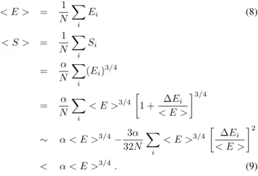
A general conclusion one can draw about this ques-tion is that the total entropy of the system becomes always smaller when one takes such fluctuations into account, in comparison to the case without fluctuations, which means with average over the event-by-event fluctuating IC taken before the expansion. This can be seen by observing that, in ideal hydrodynamics, both energy and entropy are con-served. Then, considering for simplicity an ideal gas so that Si=α(Ei)3/4, withα=const.>0, for each random event,
< E > = 1 N
i
Ei (8)
< S > = 1 N
i
Si
= α
N
i
(Ei)3/4
= α
N
i
< E >3/4
1 + ∆Ei < E >
3/4
∼ α < E >3/4− 3α 32N
i
< E >3/4
∆E
i
< E >
2
< α < E >3/4. (9)
Here, < E > and < S > in the left-hand sides mean the averaged energy and entropy over the fluctuating events, whereas the right-hand side of< S >is the entropy cor-responding to the averaged initial conditions, with the av-eraged energy< E >. The linear terms of the expansion in∆Ei/ < E >are cancelled out when the summation is performed. If one recalls that particle multiplicity is pro-portional to the entropy for each particle species, one would expect that also the multiplicity becomes, in general, smaller when one takes such fluctuations into account.
3
Equations of state
As mentioned already, the basic assumption in hydrodynam-ical models is the local thermal equilibrium. Once this con-dition is satisfied, all the thermodynamical relations should be valid in each space-time point2. Thus, the energy, pres-sure and temperature are given as functions of baryon num-ber and entropy densities, specifying the properties of the matter. In this Section, we discuss how to obtain simple phenomelogical equations of state (EoS) for the hydrody-namical description of relativistic nuclear collisions [22].
3.1
Hadronic gas
The strong interactions among hadrons are very complicated and difficult to be incorporated into the EoS for practical use. However, for very high energy, we may consider that the hadronic gas may be approximated as an ideal gas, al-though the degree of approximation can not be evaluated theoretially. The recent thermal model for the description of chemical abundances [23] show that such an approach can reproduce quite well the observed multiplicity ratios of pro-duced hadrons. Here we assume that all the particles can be treated as constituents of a quantum ideal gas, except for a correction due to the excluded volume. We also include a main part of observed resonances in Particle Data Tables. The inclusion of resonances can be considered as an effec-tive way to consider the interactions among hadrons as ex-plained later.
First, we recall that, in a grand canonical ensemble for an ideal gas of quantum particles, the thermodynamical po-tential per volume (the pressure) is given by
p(T, µ) = θ g (2π)3
d3k ln(1 +θ eβ(µ−ǫ(k)))
(10)
wereθ=±1(+for fermions,−for bosons),β = 1/T is the inverse of the temperatureT,µthe chemical potential, g the degeneracy factor andǫ(k) =√k2+m2withmthe
mass of the particle. The number densitynand the energy densityεcan be obtained by the usual thermodynamical re-lations,n= (∂p/∂µ)V,T,ε= (∂p/∂β)λ, whereλ=eβµ is the fugacity. The entropy density of the gas can be calcu-lated ass=β(p+ε−µn).
For example, in Landau’s model [1], the equation of state was taken as that of the massless pion gas. For bosons withm=µ= 0,Eq. (10) can be integrated analytically to give
p(T) =g π 2
90 T 4,
(11) and accordingly
s=g π 2
15 T
3, ε= 3p=g π2 30 T
4. (12)
For the pion gas, due to the isospin factor, we can takeg= 3.
For more realistic equations of state, we should include all the resonance particles in the gas. Furthermore, we should also take into account more than one type of con-served quantum numbers, such as electric charge (equiva-lently the 3rd component of isospin), baryon number and strangeness. In this case, the chemical potential must be written asµ = BµB +SµS +T(3)µ3 whereB, S, T(3)
are baryon, strangeness and the thrid component of isospin quantum numbers, respectively, andµB, µS andµ3are the
corresponding chemical potentials. Thus, for a mixture of particles with these conserved quantum numbers, Eq. (10) should be generalized to
pHG(T, µB, µS, µ3) =
i
pi(T, µi), (13)
where the sum refers to the particle species (including reso-nances) andµi=BiµB+SiµS+Ti(3)µ3, withBi, Si, Ti(3) the quantum numbers of thei-th particle species. We verify that the baryon number density of the mixture is
nB =
∂p ∂µB
V,T
=
i
∂p
i(T, µi)
∂µB
=
i
Bin(i), (14)
wheren(i)= (∂p
i(T, µi)/∂µi)is the number density of the
i-th particle species.
Except for pions, most of hadrons and resonances can be well approximated by the Boltzmann limit. In this case, we have
pi(T, µi)≃gi
T2m2 2π2 K2
mi
T
eµi/T, (15) and
ni=gi
T m2 2π2 K2
mi
T
eµi/T, (16) whereK2 is a modified Bessel function. From these
rela-tions, we can see immediately the usual ideal gas relation,
pi=niT . (17)
When the widths of the resonances are taken into ac-count, Eq.(13) must be modified. For an interacting gas, the power series expansion of the pressure in terms of fugacity,
p(T, µ) =pid(T, µ) +T
∞
n=2
bn(T)eβµn, (18)
is known as the cluster expansion (which is intimately re-lated with the virial expansion) andbn are called “virial” coefficients. Here,pid is the pressure of the corresponding ideal gas and, roughly speaking, the indexnin the sum rep-resents the order of multiple particle interactions. Forn= 2, the contribution to the pressure comes from the 2-body in-teractions. Beth and Uhlenbeck [24] showed that the second
2Recently it has been suggested that the thermodynamical relations can be satisfied without having the thermal equilibrium in the sense of Boltzmann
virial coefficient can be expressed in terms of the scatter-ing phase-shift of constitutscatter-ing particles. This approach was generalized to the relativistic Boltzmann gas by Dashen, Ma and Bernstein [25] and the result forb2is
b2(T) = T 2π2
∞
W0
dW W2K2(βW)
×π1 ℓ
(2ℓ+ 1) ∂
∂Wδℓ(W), (19) whereδℓ(W)is the phase shift for theℓ-th partial wave.
Consider the case of a gas of particles with massM and suppose there exists a resonance in the two particle collision,
M +M →MR. (20)
When the resonance has a widthΓand spinJ, onlyℓ=J dominates the sum and
δℓ(W) =
Γ 2
1 MR−W
, (21)
so that we have the Breit-Wigner formula, ∂
∂Wδℓ(W) = Γ 2
1
(MR−W)2+ Γ2/4
. (22)
Therefore, the pressure of the system can be written as p=pid+pR,
where pR=gR
T2Γ 4π3e
βµR
∞
W0
dW W
2K2(βW)
(MR−W)2+ Γ2/4
, (23)
with
gR = 2S+ 1,
µR = 2µ . For extremely narrow resonances,Γ→0,
pR→gR
T2M2
R
2π2 K2(βMR)e
βµR, (24) which is exactly the pressure of the ideal relativistic Boltz-mann gas made of resonances with massMR. Eq. (23) sug-gests that, for more general case, the effect of resonance width can be obtained by a convolution of the normalized mass spectrum f(M) of the resonance, with the pressure pid(M)of the ideal gas of massM, as
pR=
dMRf(MR)pid(M).
3.2
Effect of resonance width as a function of
temperature
Equation (23) shows that the effect of the resonance width on the pressure of the gas is temperature dependent. To see
this effect, let us introduce the quantity, F(T, MR,Γ) =
Γ 2πM2
RK2(MR/T) ×
∞
W0
dW W
2K2(W/T)
(MR−W)2+ Γ2/4
, (25) so that
pR=pΓ=0R ×F(T, MR,Γ). (26) Another way to see the effect of the width, we may introduce the effective mass of the resonanceMef f defined
by
Mef f2 K2(βMef f)≡MR2K2(βMR)F(T, MR,Γ). Using this effective mass, we can write the resonance pres-sure as
pR=gR
T2M2
ef f
2π2 K2(βMef f)e
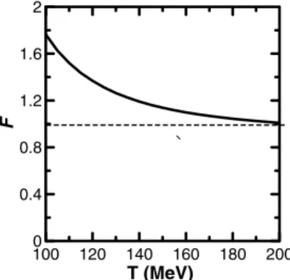
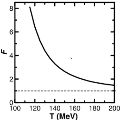
βµR, (27) that is, as if it were the pressure of ideal gas of particles with massMef f. In Figs. 3, 4, 5 and 6, we show the temperature dependence of F andMef f for two tipical cases, one for the resonanceρ(light and narrow width) and the resonance f (heavy and large width) resonances. As we see, the ideal gas approximation deviates substancially for low tempera-tures, especially for large width resonances. The ideal gas approximation is only valid forT ≫Γ.
100 120 140 160 180 200
T (MeV)
0 0.4 0.8 1.2 1.6 2
F
Figure 3. Correction factorFas function of temperatureTfor the resonanceρ.
100 120 140 160 180 200 T (MeV)
0 0.2 0.4 0.6 0.8 1
Mef
f (G
e
V
)
100 120 140 160 180 200
T (MeV)
0 2 4 6 8
F
Figure 5. Correction factorFas function of temperatureT for the resonancef.
100 120 140 160 180 200
T (MeV)
0
0.4
0.8
1.2
1.6
2
M
ef
f (G
e
V
)
Figure 6. Effective mass of the resonancefas function of temper-atureT. The dark area corresponds to the resonance width.
3.3
Excluded-volume correction
From the analysis of thermal models[23], it became clear that the ideal gas description requires a modification to ad-just the size of the system. The volume to fit the particle abundances is found to be too small. To avoid this problem, the correction due to the excluded volume effect, like a Van der Waals hard core correction is introduced [26]. Accord-ing to this prescription, Eq. (13) is modified to the followAccord-ing coupled equations
pHG(T, µB, µS, µ3) =
i=1
pid
i (T,µ˜i), (28) ˜
µi ≡ µi−vipHG, (29)
where as beforeµi=BiµB+SiµS+Ti3µ3is the chemical
potential and vi is the excluded volume of the i-th hadron species. The superscriptidrefers to the ideal gas case. The above equations constitute an implicit equation forpHG so that these two equations are solved iteratively to obtainpHG for a given set of parameters,T, µB, µSandµ3. The number
density of thei-th hadron is given by
nexcli (T, µi) =
nid
i (T,µ˜i) 1 + jvjnidj (T,µ˜j)
, (30)
wherenid
i is the ideal gas expression of the particle density for thei-th particle species.
3.4
Gas of Quarks and Gluons
The simplest way to introduce the phase of quarks and glu-ons in the equatiglu-ons of state is the use of the MIT Bag mod-els. The effect of gluon and quark condensate in the physi-cal vacuum is expressed as the energy density of the vacuum (or vacuum pressure). Thus the energy density and pressure of an ideal quark-gluon gas calculated in the QCD vacuum should be modified according to the rule,
ε → ε+B,
p → p−B,
where B is the vacuum pressure. Note that this vacuum pressure has a property analogous to the cosmological con-stantΛof Einstein. Now, when we consider just theuandd quarks and neglect their masses, we have
pqgp =
gq
6π2
1 4µ
4
q+
π2
2µ
2
qT2+ 7π4T4
60
+ gGπ
2
90 T
4−B , (31)
with
gq = 2×2×3,
gG = 2×8,
the statisfical factors of quarks and gluons. For quarks, we haveµq=µB/3.ForµB= 0,we have
p(qgpud)= 37×π
2
90T
4
−B (32) or effectivelygqgp = 37. To include the strangeness and also charge conservation, we proceed in the same way as for the hadronic gas and we have
pqgp(T, µB, µS, µ3) =
gl
6π2
1 4µ
4
u+
π2
2 µ
2
uT2+ 7π4T4
60
+ gl 6π2
1 4µ
4
d+
π2
2 µ
2
dT2+ 7π4T4
60
+pid
s(T, µs) +pids (T,−µs) +gGπ
2
90 T
4
−B , (33) wheregℓ= 2×3and
µu=
1 3µB+
1 2µ3,
µd =
1 3µB−
1 2µ3,
µs=
1
3.5
Construction of equations of state for the
practical use
The expressions Eqs. (28,29) or Eq. (33) are, however, not convenient for the use in hydrodynamical calculations. This is because the variables in such calculations are the con-served quantum numbers and the entropy density and not the chemical potentials and the temperature. So, we need to invert the relations,
nB = nB(T, µB, µS, µ3), (34)
nS = nS(T, µB, µS, µ3), (35)
n3 = n3(T, µB, µS, µ3), (36)
s = s (T, µB, µS, µ3), (37) to get
µB = µB(nB, nS, n3, s), (38) µS = µS(nB, nS, n3, s), (39) µ3 = µ3(nB, nS, n3, s), (40) T = T (nB, nS, n3, s). (41)
However, this is a formidable task even numerically. We are thus forced to reduce the degrees of freedom for the practical application to hydrodynamics. For this purpose, we set the isospin and strangeness densities to null everywhere. That is, we impose the conditions,
nS = 0, (42)
n3 = 0. (43)
These conditions together with Eqs. (35) and (36) determine µS andµ3as functions ofT andµB. Therefore,nBands in Eqs. (34) and (37) become now functions of two variables T andµB,
nB = nB(T, µB), (44)
s = s(T, µB), (45)
which can be inverted numerically and give
T = T(nB, s), (46)
µB = µB(nB, s). (47)
The above inversion process allows us to write any thermodynamic quantity as function of nB ands, both in hadronic gas and quark-gluon plasma. Then, for a given pair of density parametersnBands, we should determine which phase the physical system assumes. When two phases are in equlibrium, we must have [27]
pHG(T, µB) =pQGP(T, µB) (48) so that it determines the phase boundary line in the(µB, T) plane and separates this plane into two domains. The do-main wherepHG > pQGP is the hadron gas phase and the otherpHG< pQGP is the QGP phase. These two domains are in contact on the phase boundary line Eq. (48).
However, the above two domains in the(µB, T)plane are mapped into two separate domains in the(nB, s)plane
and there appeas a new third domain between them. That is, the phase boundary line in the(µB, T)plane spreads into a domain in the(nB, s)plane. This domain is the mixed phase. In oder to determine thermodynamical quantities in this mixed phase as functions of(nB, s), we should intro-duce another criterion in addition to the phase boundary con-dition of Gibbs. As mentioned above, any point(µB, T)on the phase boundary line corresponds to two points in the
(nB, s)plane: one for the hadron phase,(nHB, sH), and the other, (nQB, sQ), for the QGP phase. In the mixed phase, any density of extensive quantity should be a linear func-tion of the qgp/hadron concentrafunc-tion ratio. Thus for a given value of the baryon number densitynB in the mixed phase,
(nH
B, sH)and(n Q
B, sQ)should satisfy
s= s
Q −sH nQB−nH B
(nB−nHB) +sH. (49)
From this equation, we determine the two points on the phase boundaries,(nH
B, sH)and(n Q
B, sQ). All the other ex-tensive quantities, sayε, can then be obtained as
ε= ε
Q −εH nQB−nH B
(nB−nHB) +εH. (50)
Finally we can construct the equations of state in the whole region of(nB, s). The parameters of the final equa-tions of state are then,
• Number of resonances included in the hadronic gas: Here, we take all the mesons with mass smaller than 1.5 GeV, and baryons smaller than 2 GeV. Resonance widths are not included.
• Quark masses: We may safely takemu = md = 0, but for the strange quark, we takems= 120MeV. • Size of excluded volume: In the example shown in the
figures below,ν0 = (4πr30/3)withr0 = 0.7 fm for
baryons andr0= 0for mesons.
• Bag constant: We takeB = 380MeV/fm3.
Figure 7 shows the line of constant temperature in
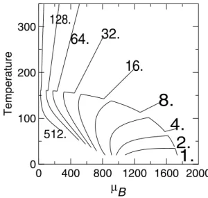
(nB, s) plane. Fig. 8 shows the lines of constant entropy per baryon in(µB, T)plane.
0
0.4
0.8
1.2
1.6
2
Baryon Number Density (1/fm
3)
04 8 12
Entropy
Den
s
ity
(1
/fm
3
)
40
160
150 140
130
120
110
100
90
80
70
60
50
Figure 7. Isotherms in the(nB, s)plane. Values of the temper-atures are indicated in the figure. Hadron gas, mixed phase and quark gluon plasma are clearly seen.
0
400
800 1200 1600 2000
µ
B
0
100
200
300
T
e
mpe
rat
u
re
512.
1.
4.
8.
16.
32.
64.
128.
2.
Figure 8. Constant entropy per nucleon curves in the(µ, T)plane. The numbers indicate(s/nB)values.
4
Resolution of hydrodynamic
equa-tions
In general, exact analytic resolution of relativistic hydrody-namics is a difficult task due to the highly non-linear na-ture of these equations. So, usually one resorts to numer-ical computations. However, since the analytnumer-ical studies
are more transparent, it would be useful to find analytical soluions, even though they correspond to highly ideal cases. Khalatnikov’s one-dimensional analytical solution [11] to Landau’s initial conditions [1], namely, ideal fluid at rest in a Lorentz contracted thin spatial region, gave rise to a new approach in high-energy physics. The boost-invariant solution [30] found 20 years later, is frequently utilized as the basis for estimations of initial energy densities in ultra-relativistic nucleus-nucleus collisions [31]. Below, we shall first describe families of analytical solutions we obtained in collaboration with T. Cs¨org˝o [32, 33].
Considering that it is not trivial to analytically solve the equations of hydrodynamics, it would be nice if we could develop a method to obtain an approximate but analytical solution of hydrodynamics. This has been done with vari-ational formulation [34], although we had not develop it further by applying it to practical problems of high-energy nuclear collisions. However, we did apply the variational method to develop a numerical code SPheRIO, based on the so-called smoothed-particle hydrodynamics (SPH) [35, 36] tecnique, to high-energy nuclear collisions [37], which is flexible enough, capable to treat systems with configurations without any symmetry and also exploding in time.
In the following, after presenting some analytical solu-tions, we shall describe in the subsection 4.2 the variational formulation of hydrodynamics, showing how it could used to get approximate solutions. Then, in the subsection 4.3, we shall apply this method to adapt the SPH hydrodynamics for relativistic heavy-ion collisions.
4.1
Analytic solutions
After Landau’s initial proposal [1], the first analytic solu-tion obtained is due to Khalatnikov [11], considering 1-dimensional expansion of ideal gas. A more simpler boost-invariant solution has been obtained later [30] and applied to estimate the initial energy densities in ultra-relativistic nucleus-nucleus collisions [31]. Both of these have been frequently used in the study of nuclear collisions, showing the usefulness of such simple analytical solutions.
However, the boost-invariant solution has some short-comings:i)it is scale invariant, having a flat rapidity distri-bution, corresponding to the extreme relativistic collisions, which has never been seen; ii) it contains no transverse flow. In [32], we tried to overcome these shortcomings. We started by assuming a simple equations of state, correspond-ing to a gas containcorrespond-ing massive conserved quanta, namely,
ε = mn+κp , (51)
p = nT , (52)
having two free parameters,mandκ. Non-relativistic hy-drodynamics of ideal gases corresponds to the limiting case ofm >> T,v2<<1andκ= 3/2.
Then, we looked forsimilarity flows,i.e.,
v =
˙ X(t) X(t)x,
˙ Y(t) Y(t)y,
˙ Z(t) Z(t)z
, (53)
f(xµ) = f
0
V
0 V
a
whereX(t), Y(t), Z(t)are the scales of length, in three or-thogonal directions, andf(xµ)is any of the thermodynami-cal quantities, such asn(xµ), T(xµ), p(xµ), . . . ,and
s= x 2
X2 + y2 Y2 +
z2
Z2 (55)
is ascaling variable.
Using this parametrization for the one-dimensional ex-pansion, it can be easily verified, by direct substitution into eqs.(1,2) with eqs.(4,51,52,53 and 55), that a family of solu-tions can be written as
v = z/t≡tanhη, n = n0(t0/τ)V(s), p = p0(t0/τ)1+1/κ, T = T0(t0/τ)1/κ
1
V(s), (56)
withp0=n0T0and whereV(s)is an arbitrary non-negative
function ofs=z2/( ˙Z2
0t2). The index0stands for the initial
values. Thus, this is a family of one-dimensional similarity flows, but it isnotscale invariant andnandT are not con-stant for a concon-stantτ.
Next, considering cylindrically symmetric flows, with boost invariance alongzdirection (collision axis), we could find the following family of solutions, for transverse flows:
v = r/t , for |r| ≤t, n = n0(τz0/τ))3V(s), p = p0(τz0/τ)3+3/κ, T = T0(τz0/τ))3/κ 1
V(s). (57)
Here,p0=n0T0andV(s)is an arbitrary non-negative
func-tion ofs(=r2
t/( ˙R02τz2) in this case), withrt=
x2+y2
andR˙0 =
˙ X2
0+ ˙Y02 andτz = √
t2−z2. So, this is a
generalization of the one-dimensional scale-invariant solu-tion, including a class of transverse flows.
More recently [33], we extended these solutions still fur-ther, considering less symmetrical flows, but still keeping the same EoS (1,2) and similarity flow, with constant veloc-ity, as it appears in eqs.(56,57).
4.2
Variational formulation
As shown above, even for very simple equations of state, an-alytic solutions are limited to special cases. For realistic sit-uations, even the equations of state themselves are available only in the form of numerical tables. Therefore, the numer-ical resources are essential for realistic studies of hydrody-namical behavior of ultra-relativistic collisional processes. However, it is well-known that any numerical method for partial differencial equations requires highly sophisticated techniques to avoid numerical instabilities, and usually it needs a very large scale computation, especially when we want to describe correctly explosive processes such as rela-tivistic heavy-ion collisions. However, as emphasized in the
Introduction, in the hydrodynamic approach of high-energy nuclear collisions, its main ingredients, i.e., the equations of state, the initial conditions and the freezeout conditions are not quite well known. In such a situation, we actually don’t need a very precise solution of the hydrodynamic equations, but a general flow pattern which characterizes the final con-figuration of the system as a response to given equations of state, initial conditions and the decoupling procedure. So, we prefer a rather simple scheme of solving the hydrody-namic equations, not unnecessarily too precise but robust enough to deal with any kind of geometry. From this point of view, we stressed in Ref. [34] the advantage of a varia-tional approach to relativistic hydrodynamics.
Although not commonly found in general textbooks, the variational formulation of hydrodynamics has been studied by several authors [38, 39]. In Ref. [34], starting from the action
I=
d4x{−ε}, (58)
whereεis the proper energy density, the relativistic hydro-dynamics was derived from the variational principle.
Here, we show its derivation, generalizing to include the rotational flow. To do this, we introduce the two variables, the proper baryon density,n, and entropy density,s, which satisfy the conservation laws,
∂µ(nuµ) = 0,
∂µ(suµ) = 0. (59) whereuµis the four velocity of the fluid, satisfying the nor-malization,
uµuµ = 1. (60)
The functional form of the energy density, ε=ε(n, s),
specifies the thermodynamical properties of the fluid. The pressure, temperature and chemical potential are obtained by the usual thermodynamic relations,
p = n∂[ε(n, s)/n]
∂n ,
T = ∂ε(n, s)
∂s and
µ = ∂ε(n, s)
∂n .
The hydrodynamical equations of motion for the fluid is given by the variational principle with respect ton, sand uµunder the constraints, Eq. (59), and the normalization of the four-velocity, Eq.(60). These constraints can be incor-porated in the variational principle in terms of Lagrangian multipliers to write
δ
d4[ − ε(n, s) +λ∂µ(nuµ) +ζ∂µ(suµ)
− 1
2w(u
µu
whereλ, ζ andware Lagrangian multipliers and arbitrary functions ofx. Equivalently, the fluid dynamics is given by the effective Lagrangian,
L(ef ff luid)(n, s, uµ, λ, ζ, w) = − ε(n, s)−nuµ∂µλ − suµ∂
µζ−
w 2(u
µu µ−1),
(62) where now all of n, s, uµ, λ, ζ, w are independent varia-tional variables.
The variations with respect ton, sanduµlead immedi-ately to
−µ−uµ∂µλ = 0, (63) −T−uµ∂µζ = 0, (64) −n∂µλ−s∂µζ−wuµ = 0. (65) Variations with respect toλ, ζ andwgive simply the con-straints, Eqs. (59) and (60). Multiplying the both sides of Eq.(65) byuµ, and using Eqs. (60,63,64), we get
w = nµ+T s
= ε+p , (66)
wherepis the pressure. Eq.(66) shows thatwis the enthalpy density. Substituting back thiswinto Eq.(65) and multiply-ing byuν, we have
wuµuν=−(nuν)(∂µλ)−(suν)(∂µζ).
Taking the divergence and using the continuity equations ∂ν(nu
ν) = 0and∂ν(suν) = 0, we get
∂ν(wuµuν) =−(nuν)(∂ν∂µλ)−(suν)(∂ν∂µζ). (67) But
(nuν)(∂ν∂µλ) = n∂µ(uν∂νλ)−n(∂νλ)(∂µuν)
= −n∂µµ−n(∂νλ)(∂µuν) and analogously
(suν)(∂ν∂µζ) =−s∂µT −s(∂νζ)(∂µuν), so that Eq.(67) becomes
∂ν(wuµuν) = n∂µµ+s∂µT+ (∂µuν)wuν
= ∂µp+uν(∂µuν)w
= ∂µp . (68)
Here, we have used Eq.(65) and the Gibbs-Duhem relation,
dp=sdT+ndµ , (69)
and the property,
uν(∂µuν) = 0.
Finally we arrive at the standard form of the relativistic hy-drodynamic equation (1),
∂νTµν = 0, (70)
where
Tµν = wuµuν−gµνp
= (p+ε)uµuν−gµνp (71)
is the usual energy-momentum tensor of the fluid.
It is important to observe that, the effective Lagrangian Eq.(62) evaluated in the proper comoving frame of the fluid motion is
L(ef ff luid)
comoving=−ε(n, s) +µn+T s=p , (72)
which is nothing but the negative of the thermodynamic po-tential of the fluid element atxµ.
Now, interesting application of this approach appears, if we can parametrize possible solutions of continuity equa-tions (59) in terms of a certain number of time-dependent parametersa(t) ={ai(t), i= 1, . . . , N}, such that
n = n
r, a(t),da(t) dt
,
s = s
r, a(t),da(t) dt
,
together with the velocity field,
uµ=uµ
r, a(t),da(t) dt
,
then the action, Eq. (58), may be written as a time integral of an effective Lagrangian
Lef f
a(t),da(t) dt
=−
drε(n, s). (73)
The constraint terms vanish for these ansatz. In this case, the equations of motion for the variablesai(t)are obtained as the Euler-Lagrange equations. This method could be ap-plied to relativistic heavy-ion collisions, trying to describe them in a simple analytic and effective way in terms of few parameters. However, the general parametrization which solve exactly the continuity equations is not easy. An ap-proximate way to solve the continuity equation is proposed in a numerical method calledSmoothed Particle Hydrody-namics.
4.3
Smoothed particle hydrodynamics
4.3.1 SPH representation of densities
The basic idea of the SPH method is to parametrize the con-tinous density distribution of any extensive physical quantity in terms of sum of base functions with finite support. This procedure introduces two types of approximations of differ-ent nature. To see this, let us suppose thatAis the physical extensive quantity anda(r, t)the corresponding density dis-tribution. We start with the identity,
a(r, t) =
a(r′
, t)δ(r−r′ )d3r′
.
Now, let us introduce the first approximation. Substitute the Diracδ-function by a smooth, normalized functionW with finite support, say,h, and transform the densityatoaas
a(r, t)→a(r, t) =
a(r′
, t)W(r−r′ ;h)d3r′
, (74) where as mentioned,W is normalized,
W(r−r′ ;h)d3r′
= 1.
and having the property of finite support, W(r−r′
;h)→0, for|r−r′
|> h .
At this stage, the new densitya(r, t)describes the smoothed part of the original densitya(r, t). From the Fourier trans-form, we can see that for this smoothed density, the Fourier components with large wave numbers, corresponding to
k > 1 h ,
vanish rapidly. In other words, the kernel functionWserves as the short wavelength cut-off filter. Physically, it is useful to introduce such a filter, since we very often want to elim-inate very short scale part in order to extract the global fea-ture of the dynamics of the system. In 60’s, similar idea has been used to smooth out the spectrum density of the nuclear shell model to extract the collective liquid drop potential by Strutinski [40].
Now, we introduce the second approximation. This is rather to do with the practical aspect, that is, to reduce the degrees of freedom involved in the calculation. We replace the integral Eq.(74) by the sum over a finite and discrete set of points,{ri, i= 1, .., N}.
a(r, t)→aSP H(r, t) = N
i
AiW(r−ri;h), (75)
where the weightAishould be chosen appropriately to min-imize the difference betweena(r, t)andaSP H(r, t) every-where. The above expression means that we are represent-ing the continuous density as due to a sum of a finite number of dynamic units carrying the quantityAi. These units are centered at the positionri.
Finally, the correspondence,
a(r, t)→aSP H(r, t) = N
i
AiW(r−ri;h) (76)
can be considered as an approximation ansatz for the den-sitya(r, t)with a finite number of parameters,{Ai,ri, i=
1.., N}. Due to the normalization of the kernelW, we have
aSP H(r, t)d3r= N
i
Ai,
so that we should choose N
i
Ai
as the total value of the quantityAof the system.
4.3.2 Solution of continuity equations
For the application in Hydrodynamics, we can use these pa-rameters as the variational variables so that they are time dependent. When we deal with one or more extensive quan-tities, we usually choose one conserved quantity as the refer-ence density, sayρ, and represent it by the SPH form, choos-ing appropriately the weights{νi}to get
ρSHP(r, t) = N
i
νiW(r−ri(t);h), (77)
and takeνi constant in time. Other extensive quantity, say
A, is calculated as in Eq.(76) with weights,
Ai=
a ρ
i
νi. (78)
The quantity(a/ρ)i then represents the quantity Afor the unit reference quantityρat the positionr=ri(t). Note that the time dependence of the density in Eq.(77) comes from those of{ri(t)}. In this sense, Eq.(77) can be understood as if{ri(t)}were Lagrangian coordinates attached to small volumes of the order ofh3,with some conserved quantity,
such as baryon number or entropy in the adiabatic expan-sion. From now on, we refer to these dynamic units char-acterized by their coordinates{ri}and carrying the quantity
Aias “SPH particles”. From Eq.(78), the quantityAican be interpreted as the part ofAcarried by thei-th SPH particle. The most powerful point of the above scheme of SPH representation is that we can solve the continuity equation in a very simple manner. SupposeM is a conserved quan-tity. Then the corresponding density ρ should satisfy the continuity equation,
∂ρ(r, t)
∂t +∇ ·(ρv) = 0, (79) wherev is the velocity field. The SPH expression for the currentj=ρvis
jSP H(r, t) =
i
so that
∇ ·jSP H(r, t) =
i
viνi∇W(r−ri).
On the other hand, from Eq.(77), ∂ρSP H(r, t)
∂t =
i
νi
d
dtW(r−ri(t))
=
i
νid ri(t)
dt · ∇W(r−ri(t)), By inspection, if we identify
vi=
dri(t)
dt ,
then we can see that Eq.(79) is automatically satisfied. For the application to the relativistic heavy ion colli-sions, we can take the entropy and baryon number as the ba-sic conserved quantities. Then, their densities (in the space-fixed frame) are parametrized as
s∗
(r, t) =
N
i
νiW(r−ri(t)), (80)
n∗
(r, t) =
N
i
biW(r−ri(t)), (81)
whereνiandbiare the entropy and baryon number attached to thei-th “particle”. The total entropy and baryon number are then given by
S =
d3rs∗ (r, t) =
N
i
νi. (82)
B =
d3rn∗ (r, t) =
N
i
bi. (83)
The proper densities of entropy and baryon number are re-lated with these space-fixed frame quantities as
s = γ−1s∗
, n = γ−1n∗
,
whereγ=u0is the Lorentz factor asscociated with the fluid
velocity. For the hydrodynamical description of nuclear and hadronic collisions at ultra-relativistic energies, we prefer to use the entropy than the baryon number as the reference conserved number to write the SPH representation of any other extensive quantities. This is because, the baryon den-sity may become zero but the entropy denden-sity never vanishes in the physically interesting region within a hydrodynamical description.
4.3.3 SPH action and SPH equations
In the variational derivation of this method, the set of time-dependent variables{ri, i= 1, ..., n}are taken as the vari-ational degrees of freedom and their equations of motion
are determined by minimizing the action for the hydrody-namic system. Thus, SPH may be considered as an effec-tive description, in which the coordinates{ri(t)}associated with “particles” are the optimal dynamical parameters which minimize the model action. We observe that{νi}or{bi}are not dynamical variables and are determined by the initital conditions together with the constraints for the variational procedure.
The effective Lagrangian, Eq. (73), is rewritten in SPH representation as
LSP H({ri,˙ri}) =−
i
νi(ε/s∗)i=−
i
E γ
i
,
(84) whereEiis the “rest energy” of thei-th “particle”. Then, the equations of motion are obtained from the usual variational procedure. This leads to the following coupled equations
d dt
νi
pi+εi
si
γivi
+
j
νiνj
p
i
s∗
i2
+ pj s∗
j2
∇iW(ri−rj;h) = 0.
(85) 4.3.4 General coordinate system
The variational procedure can readily be extended to coor-dinate system, with a non-Cartesian metric. The use of gen-eralized coordinate systems is particularly important when we consider realistic initial conditions for simulations of RHIC processes. As we know, in a relativistic heavy-ion collisional process, the initial state is a cold, quantum nu-clear matter. Just after the collision, the hadronic matter stays at a highly off-shell state and the materialization oc-curs only after∼1fm/c in the proper time. Therefore, the local thermodynamical state would emerge for some local proper time and not for the global space-fixed timet. Thus, it is important to choose a convenient coordinate system for the description of the relativistic heavy-ion collisions. For example, one often uses the hyperbolic time and longitudi-nal coordinates to be described later.
Let us consider a general coordinate system, with
ds2=gµνdxµdxν. (86)
However, in order to unambiguously define the conserved quantity, we consider only the case where the time-like co-ordinate is orthogonal to the space-like coco-ordinates,
gµ0= 0. (87)
The action principle for the relativistic fluid motion can be written as [34]
δI=−δ
d4x√−g ε= 0, (88)
together with the constraint for the conserved entropy cur-rent,
(suµ);µ=
1
√ −g∂µ(
√
or
1
√ −g∂τ
√
−gsγ+√1 −g
i
∂i√−gsγvi= 0, (90)
where
vi= u
i
u0 (91)
and we use the notation
τ =x0, γ=u0.
The generalized gamma factorγis related to the velocityva throughuµuµ = 1, so that
γ= 1
g00−vTgv
, (92)
where−gis the3×3space part of the metric tensor. That is
(gµν) =
g00 0
0 −g
. (93)
Let us now introduce the SPH representation. We may, for example, express the entropy density by the ansatz
√
−gsγ=s∗
→ s∗
SP H =
i
νiW(r−ri(τ)), (94)
or by
sγ=s∗
→s∗
SP H=
i
νiW(r−ri(τ)) (95)
as well. These two possibilities, besides others, are simply different ways to parametrize the variational ansatz in terms of a linear combination of given functionsW(r−ra(τ)). The most important property of an ansatz should be thatW satisfies the normalization condition imposed by the basic conserved quantity. Since the total entropy is expressed as
S=
d3r√−g sγ=
i
νi, (96)
the normalization ofW should be taken to be
d3r W(r−r′
) = 1, (97)
for the parametrization Eq.(94) and
d3r√−gW(r−r′
) = 1, (98)
for the parametrization Eq.(95). In the usual SPH calcula-tions, it is not desirable to introduce inW the space-time dependence through its normalization condition. In this re-spect, the most natural way to introduce the SPH represen-tation is Eq.(94). With this choice, the SPH action is given by
ISP H = −
dτ
d3r
i
νi
√ −g ε √
−g sγ
i
W(r−ri(τ))
= − dτ i νi ε sγ i . (99)
The variational principle leads to the following equation of motion,
d
dτπi= −
j
νiνj
1
√ −giγ2i
pi
s2
i
+√ 1 −gjγ2j
pj
s2
j
∇iWij
+ νi γi pi si 1 √ −g∇
√ −g
i
+ νi 2γi
p+ε
s
i
(∇g00−viT∇gvi), (100)
where
πi=γiνi
p+ε s
i
gvi (101)
and the operator∇is just the simple derivative operator with respect to the coordinate variables in use.
For ultrarelativistic heavy-ion collisions, a useful set of variables is
τ = t2−z2, (102)
η = 1
2tanh t+z
t−z, (103)
rT =
x y
. (104)
As mentioned above, the initial conditions for RHIC processes are specified in terms of the proper time rather than of the fixed-frame timet. The variableτ is not exactly the physical proper time of the matter, but in general it is a good approximation in ultra relativistic collisions.
The metric tensor for this coordinate system is given by g00 = 1,
g =
1 0 0
0 1 0
0 0 τ2
,
√
−g = τ .
Since the metric is space independent, we can use the para-metrization
τ γisi=s
∗
i = n
j=1
νjW(qij),
where qij=
(xi−xj)2+ (yi−yj)2+τ2(ηi−ηj)2
andWis normalized as
4π
∞
0
The SPH equation becomes d
dτπi=− 1 τ
j
νiνj
1 γ2
i
pi
s2
i
+ 1 γ2
j
pj
s2
j
∇iWij,
where theη component of the momentum is related to the velocitydη/dτ as
πη =τ2νγ
p+ε
s
dη
dτ,
whereas in the transverse direction, we have πT =νγ
p+ε
s
dr
T
dτ .
The Lorentz factor is given by
γ= 1
1−v2
T−τ2vη2
.
4.3.5 Landau Model
In order to show the efficiency of the method and also to show the correct choice of the coordinate system, let us in-vestigate the Landau model in the SPH scheme, using the ordinary Cartesian coodinates andη−τcoodinates. Since the analytical solution is known, we can compare the numer-ical solutions to it.
We thus solve the hydrodynamical evolution of a system of one-dimensional relativistic massless baryon-free gas ini-tially at rest. The equation of state of a relativistic massless boson gas is
p= 1 3ε=Cs
4/3,
where
C=
15
128π2
1/3 .
To apply the SPH method, we introduce the discrete one-dimensional space variablexi(t), i= 1, .., n(and similarly forη−τcoodinates). The relation between the momentum and velocity is then
π= 4Cνs∗1/3γ2/3v,
(105) where, in this case,vcan be solved analytically with respect toπ.
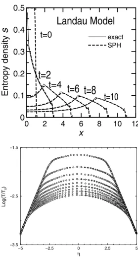
In Figs. 9 a and b, we show the results of our SPH cal-culation together with the exact solution [11,1]. In these examples, we took only 100 particles with equally spaced xi (orηi). As we see from this example, in spite of rather small number of particles, the SPH solution is quite satis-factory. In particular, when we use the η−τ coordinates with an appropriate distribution ofν′
is(Fig. 9 b), an excel-lent agreement with the analytical solution can be obtained. The computation time needed to get these solutions is even less than that needed to numerically evaluate the analytical solution.
0 2 4 6 8 10 12
x
0
0.1
0.2
0.3
0.4
0.5
Entropy de
n
s
ity
s
exact SPH
Landau Model
t=0
t=2
t=4
t=6
t=8
t=10
−5 −2.5 0 2.5 5
η
−3.5 −2.5 −1.5
Log(T/T
0
)
Figure 9. a) (above) Entropy profiles of the Landau model in Cartesian coordinate for different times. The exact results are given by the broken curves. The SPH solution is shown by the full curves.
b)(below) Temperature profiles of the Landau model in the hyper-bolic coordinate system (see text), for different timeτ. The SPH calculation is represented by the circles, and the exact result by the broken curves.
4.3.6 Transverse expansion on longitudinal scaling ex-pansion
0 10 20 r
0 0.1 0.2 0.3 0.4
T/T
0
τ=5.0
τ=1.0
τ=10.0
τ=15.0
Figure 10. Temperature profile of a cilyndrically symmetric flow with longitudinally scaling expansion, shown as a function of
r = p x2+y2. The SPH results atη = 0(circles) are
com-pared with the numerical solution obtained by a space-fixed grid method [41]. The SPH calculation has been perfomed in full 3D.
4.3.7 Shock formation and Neumann-Richtmyer pseudo viscosity
As seen in the previous examples, our entropy-based rela-tivistic SPH method works quite well for the adiabatic dy-namics of the massless pion gas. However, for the applica-tion to realistic problems, it is fundamental to see how this scheme works for non-adiabatic cases, too. This is because, whenever a piece of fluid matter flows into another region of the fluid with a speed exceeding the sound velocity of the fluid, there appears a shock wave, and this is essencially a nonadiabatic process. Thus, except for a really quasi-static dynamics, there should be an entropy production mecha-nism. This becomes especially important in a domain close to the phase transition region, because there the velocity of sound tends to zero. In the following, we study some ex-amples of one dimensional shock problems in the scheme of the SPH methods.
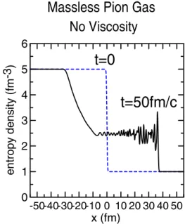
The shock front manifests as a discontinuity in thermo-dynamical quantities in a hydrodynamic solution. Math-ematically speaking, the shock front should be treated as a boundary connecting two distinct hydrodynamic solu-tions. The smoothed particle ansatz excludes such a pos-sibility from the beginning. Since short-wavelength excita-tion modes do not exist in the SPH ansatz, the energy and momentum conservation required by the hydrodynamics re-sults in very rapidly oscillating motion of each SPH parti-cle. Such a situation occurs, for example, when a very high-energy density gas is released into a low density region. This kind of shock, for the case of a baryon gas, is discussed in [42] and also, in the SPH context, in [43]. Here, we ap-pliy our entropy-based SPH approach to the massless pion gas.
Figure 11 gives the typical behavior of SPH solution for such a situation, if entropy production is not taken into ac-count. As discussed above, there appear in fact rapid oscil-lations in thermodynamical quantities just behind the shock front. Actually, such oscillations always appear in any nu-merical approach if entropy production is not included.
-50-40-30-20-10 0 10 20 30 40 50
x (fm)
0
1
2
3
4
5
6
entropy d
ensity
(fm
-3
)
No Viscosity
Massless Pion Gas
t=0
t=50fm/c
Figure 11. Shock wave formation in one-dimensional pion gas, calculated with SPH. No viscosity is used.
In order to avoid these unphysical oscillations, von Neuman and Richtmyer [44] introduced the concept of pseudoviscosity. The idea is to set the dissipative pressure where the shock wave discontinuity is present. To do this, Neuman and Richtmyer proposed to replace the pressure by
p→p+Q,
whereQis the pseudoviscosity and they took the following ansatz,
Q=
(α∆x)2ρ( ˙ρ/ρ)2, ρ >˙ 0
0, ρ <˙ 0 .
The above formula is for nonrelativistic one-dimensional hydrodynamics. Here,ρis the mass density,∆xis the space grid size andαis a constant of the order of unity. In order to generalize the above pseudoviscosity for relativistic SPH case, we replace the quantityρ/ρ˙ by−θ=−∂µuµand∆x byh, wherehis as before the width of the smoothing kernel W. More precisely, we take the following form which is a slightly modified expression suggested by Ref. [43],
Q=
p−αhθ+β(hθ)2, θ <0,
0, θ≥0. (106)
where
θ= 1 V
dV dt
=∂µuµ. (107)
and the internal thermal energy is still conserved. In order to incorporate the internal energy conservation in the SPH scheme, we substitute all the pressurepibypi+Qi,and we add the following equation for the entropy production,
1 νi
dνi
dt =− Qiγi
T s∗
i
θi. (108)
-50-40-30-20-10 0 10 20 30 40 50
x (fm)
0
1
2
3
4
5
6
entropy d
ensity
(fm
-3
)
With Viscosity
Massless Pion Gas
t=0
t=50fm/c
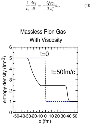
Figure 12. After the introduction of theQterm in the SPH calcu-lation.
Figure 12 is the solution of the same problem as in Fig. 11, but with the entropy production taken into account. In this calculation, the parameters have been chosen as
α= 2, β= 4
and h = 0.5f m for 1000 SPH particles. As we see, the rapid oscillations have been smoothed out (and in turn, the numerical calculation became much more efficient).
It is known that the energy- and momentum-flux conser-vations through a shock front relate the ratios2/s1 of
en-tropy densities after and before the shock to the velocityvs of the shock front as (Hugoniot-Rankine relation)
s2 s1 =
2 33/4vs
(9v2
s−1)1/4
(1−v2
s)5/4
. (109)
In Fig. 13, we show the velocity of the shock front ob-tained in our SPH calculations as function of the entropy ratio(dots). Each point corresponds to the different initial condition. They are compared with the Hugoniot-Rankine relation Eq. (109) (curve). The accordance shows that our SPH calculation reproduces faithfully the conservation of kinetic energy and momentum of the flow through the shock front.
1
2
3
4
5
6
7
8
Ratio of entropy densities
0.5
0.6
0.7
0.8
0.9
1
Shock velocity /
c
Hugoniot-Rankine Relation
Figure 13. Test of Hugoniot-Rankine relation. The circles are re-sults of SPH calculations with different initial conditions, and the full curve is Eq. (109).
In the usual hydrodynamic computations using space grids, the symmetry of the problem is often a crucial factor to perform a calculation of reasonable size. The SPH method cures this aspect and furnishes a robust algo-rithm particularly appropriate to the description of processes where rapid expansions of the fluid should be treated. The equations of motion are derived by a variational procedure from the SPH model action with respect to the Lagrangian comoving coordinates. This guarantees that the method fur-nishes the maximal efficiency for a given number of degrees of freedom, keeping strictly the energy and momentum con-servation. For this reason, solutions can be obtained with a very reasonable precision, with a relatively small number of SPH particles. This is the basic advantage of the present method, when we analyze the event-by-event dynamics of the relativistic heavy-ion collisions.
On the other hand, the precision of this method increases rather slowly with the number of SPH particles. Therefore, a relatively large number of particles is required if one wants a very precise numerical solution. However, for the appli-cation to the RHIC physics, we may need rather crude pre-cision especially if we consider the dubious validity of the rigorous hydrodynamics. For a calculation with typically
10%errors, the SPH algorithm presented here furnishes a very efficient tool to study the flow phenomena in the RHIC physics.
A fundamental difficulty of the relativistic hydrodynam-ics for viscous fluid [45, 46] is that the dissipation term causes an intrinsic instability to the system. This instability basically comes from the fact that the dissipation term con-tainsθ = ∂µu
by introducing higher-order thermodynamics with respect to deviations from the equilibrium. Recently this “second or-der thermodynamics” formalism was discussed in the con-text of Bjorken type solution [47]. In the examples presented in the present paper, we did not address this question and simply estimated the quantityθfrom the quantities one time step before. In practice, this will cause no numerical insta-bility and the behavior of the solution is quite satisfactory.
In spite of the above conceptual difficulties when nona-diabatic process is involved, the SPH approach has a nice feature as its flexibility, allowing the treatment of problems with initial conditions without any symmetry, as happens in small systems as those resulting in relativistic nuclear col-lisions. It should be stressed that, due to the use of La-grangian coordinates, the method is most suitable for ex-plosive processes like the relativistic heavy ion collisions. (Lagrangian coordinates have been used for treatment of relativistic nuclear collisions also by Nonaka, Honda and Muroya [14]). Furthermore, the variatioal approach guaran-tees that the SPH equations (85) give the optimal description of motions for a given total number of “particles”{ri(t)}, which are our parameters. In this approach, no numerical in-stabilities will occur, since the whole system is a Lagrangian system. A numerical code, called SPheRIO has been devel-opped by us on the basis of this algorithm. We shall discuss, in Sec.6, some results obtained using this code.
5
Decoupling criteria
5.1
Cooper-Frye prescription
As mentioned in the Introduction, the decoupling process is customarily described using the Cooper-Frye prescrip-tion [7], which gives the invariant momentum distribuprescrip-tion as
Ed 3N
dp3 =
σ
dσµpµf(x, p). (110) This description of decoupling introduces a sharp freezeout hypersurfaceσ, usually characterized by a constant temper-ature Tf.o.. Before crossing it, particles have a hydrody-namical behavior and, when they cross itsuddenly decou-ple, free-streaming toward the detectors, keeping memory of the conditions (flow, temperature) of where and when they crossed the three dimensional surface.
In SPH representation, we write Ed
3N
dp3 =
j
νjnjµpµ
sj|njµuµj|
f(ujµpµ), (111)
where the summation is over all the SPH particles, which should be taken where they cross the hyper-surface T = Tf.o. andnjµis the normal to this hyper-surface.
Another often used procedure is to take such a freezeout temperature not only constant for a given energy but also energy-independent.
Though operationally simple, and actually useful for ob-taining a nice comprehension of several aspects of the phe-nomena, such a concept of sharp freezeout hypersurface and
also of a constant freezeout temperature are clearly highly idealized when applied to finite-volume and finite-lifetime systems as those formed in high-energy heavy-ion colli-sions.
5.2
Finite-size effect
Before going further, let us for a moment assume that such a freezeout temperature is meaningful. At least, as an average temperature, it should exist. Then, how can we estimate it based on the properties of the system? A simple and natural criterion has already been given by Landau [1], by which a particle decouples when its mean free-pathℓin the medium becomes larger than the system sizeL,
ℓ > L . (112)
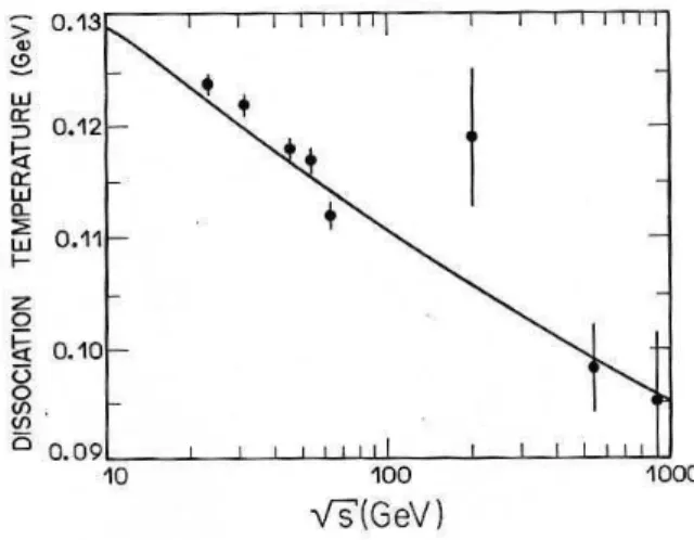
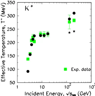
This means that Tf.o. is not an intrinsic thermodynamic property of the fluid, but it depends also on the size of the system. In [48], we applied this idea to estimateTf.o. as function of the incident energy both forpp(pp¯ ) and nucleus-nucleus collisions, obtaining approximately
Tf.o.∼(√s)
−1/12.
(113) Here, the energy dependence appears as a consequence of the increase in the initial energy density, which implies longer expansion time, so larger sizeLof the system (both longitudinally and tranversally) at the moment of decou-pling, requiring lower density, so lower decoupling temper-ature, too. Fig. 14 shows the comparison made in [48] of an estimate of the incident-energy dependence ofTf.o., using Landau’s criterion mentioned above, withTf.o. obtained in a data analysis ofπandKtransverse-momentum spectra in pp(andpp¯ ) collisions, in terms of a hydrodynamic parame-trization of transverse velocity distribution and temperature. The data were taken from [49, 50, 51].