E
NERGY AND
E
NVIRONMENT
Volume 1, Issue 1, 2010 pp.97-112
Journal homepage: www.IJEE.IEEFoundation.org
Dispersion modeling in assessing air quality of industrial
projects under Indian regulatory regime
Amitava Bandyopadhyay
Department of Chemical Engineering, University of Calcutta, 92, A.P.C.Road, Kolkata 700 009, India.
Abstract
Environmental impact assessment (EIA) studies conducted over the years as a part of obtaining environmental clearance in accordance with Indian regulation have been given significant attention towards carrying out Gaussian dispersion modeling for predicting the ground level concentration (GLC) of pollutants, especially for SO2. Making any adhoc decision towards recommending flue gas desulfurization (FGD) system in Indian fossil fuel combustion operations is not realistic considering the usage of fuel with low sulfur content. Thus a predictive modeling is imperative prior to making any conclusive decision. In the light of this finding, dispersion modeling has been accorded in Indian environmental regulations. This article aims at providing approaches to ascertain pollution potential for proposed power plant operation either alone or in presence of other industrial operations under different conditions. In order to assess the performance of the computational work four different cases were analyzed based on worst scenario. Results obtained through predictions were compared with National Ambient Air Quality Standards (NAAQS) of India. One specific case found to overshoot the ambient air quality adversely in respect of SO2 and was therefore, suggested to install a FGD system with at least 80 % SO2 removal efficiency. With this recommendation, the cumulative prediction yielded a very conservative resultant value of 24 hourly maximum GLC of SO2 as against a value that exceeded well above the stipulated value without considering the FGD system. The computational algorithm developed can therefore, be gainfully utilized for the purpose of EIA analysis in Indian condition.
Copyright © 2010 International Energy and Environment Foundation - All rights reserved.
Keywords: Environmental clearance, Environmental impact assessment, Flue gas desulfurization, Gaussian dispersion modeling, Industrial projects, Power plant operation.
1. Introduction
Forests (MoEF), Government of India decided to put forward dispersion model for assessing the emission of air pollutants from multiple point sources. The main objectives of this dispersion model were to provide an insight to atmospheric contamination process, to promote understanding on pollution dispersion mechanism, to suggest rational approaches to translate complex physical phenomena governing pollution dispersion processes in appropriate mathematical formulation amenable to numerical solution and finally the development of a computational tool in the form of a software for serving the designers in evaluating the effect of power plant operations on the ambient air quality in terms of concentration level of various pollutants.
components and processes for instance, an integrated adaptive network of sensors for environmental monitoring; a set of distributed databases for data management; a set of intelligent models for environmental modelling; a set of efficient user interfaces for data access; and a reliable, high capacity, high performance computing and communication infrastructure for integrating and supporting other framework components and processes. Carmichael et al. [9] reported on the advances in air quality forecasting with an emphasis on data assimilation. Applications of the four-dimensional variation method (4D-Var), the ensemble Kalman filter (EnKF) approach and the computation challenges were elucidated. Elkamel et al. [10] investigated on the impact of multiple pollutants (i.e., CO, NOx and SO2) emitted from different sources within a given area on the ambient air quality. An interactive optimization methodology was used for allocating the number and configuration of an Air Quality Monitoring Network. A mathematical model based on the multiple cell approach was used to create monthly spatial distributions for the concentrations of the pollutants emitted from different point sources. The model was tested to refinery stacks and results indicated that three stations could provide a total coverage of more than 70%. Ainslie and Jackson [11] investigated the methods for determining the adverse effects of air emission from potential burning of isolated piles of mountain pine beetle-killed lodge pole pine in the city of Prince George, British Columbia, Canada. The CALPUFF atmospheric dispersion model was used to analyze to identify safe burning regions based on atmospheric stability and wind direction. Reportedly, model results showed that the location and extent of influence regions was sensitive to wind speed, wind direction, atmospheric stability and a threshold used to quantify excessive concentrations. Critical appraisal of the existing literature indicates that such a traditional statistical approach using the Gaussian-type dispersion model has thus far been used extensively for carrying out environmental impact assessment (EIA) studies of several industrial projects.
Attempts have been made in this article to demonstrate the features of a computational algorithm that is developed [12] based on Gaussian dispersion to assist the policy makers, planners, designers in evaluating the effect of stationary point sources as in the emissions occurring from the stack of a coal fired thermal power plant on the surrounding ambient air quality in terms of ground level concentration of pollutants, especially for SO2. The necessities of conducting such study are to:
• Identify plausible impacts of air pollutants emitted from stationary point source from an industry on surrounding ambient air quality.
• Characterize the design modifications in achieving improved ambient air quality.
• Identify plausible site for establishment of proposed industrial activity.
• Assess the carrying capacity of a place intended for industrial activity leading to point source air emission and hence to evaluate the suitability of a site to accommodate new industries.
To characterize the fundamental features of this algorithm some case studies are described taking into consideration of few power projects and a sponge iron plant those are being planned for establishment. Though the numerical computation method developed based on Gaussian dispersion modeling for power plants and a sponge iron plant, it can also be applicable to host of other industrial operations having the potential to generate air pollutants through point stationary sources.
2. Modeling of air pollution dispersion: Indian development
3. Guidelines of MoEF for Gaussian dispersion modeling
The guidelines for EIA studies put forward by the CPCB of India under the aegis of MoEF are discussed here in this section. The guidelines recognized the urgent need for developing an exhaustive data bank on meteorological parameters and also recommended methodologies to estimate various parameters governing atmospheric dispersion process. However, these guidelines were termed as purely tentative and emphasis was given for carrying out continuous monitoring of the relevant parameters emitting from the industrial operation on surrounding air quality in order to assess the situation rigorously for arriving at methodologies suitable for Indian conditions. The parameters in these guidelines are presented below:
Design parameters: These data are based on 100% plant capacity, fuel consumption rate, fuel analysis data, flue gas velocity, stack gas temperature, flue gas flow rate, density of flue gas, specific heat of flue gas, heat emission rate of flue gas at the top of the stack, buoyancy or momentum flux parameter, control device for the particulate matter collection and its efficiency of collection.
Emission rate: Emission rates of pollutants are to be calculated assuming 0.5% S-content, if % S-content is not greater than 0.5%; If % S-content > 0.5% then actual value to be considered; for particulate emission, the collection efficiency of the electrostatic precipitator along with the emission standard for PM to be used.
Meteorological parameters: Wind speed, wind direction (for hourly and half hourly mean values) are to be generated for all seasons in a year.
Site specific data: Ambient temperature, humidity, cloud cover, solar insolation, precipitation (monthly total, number of rainy days > 2.5 mm/day), barometric pressure.
Stability class: Pasquill-Gifford Stability Classification is to be used.
Wind speed: Irwin power law velocity profile is to be used for extrapolating wind speed. Mixing height: Site-specific data are to be used as per availability or to be generated. Plume rise:Briggs Plume rise equation with modification is to be used.
Urban-rural classification:When more than 50% land inside a circle of 3 km radius around the source comprises industries, commercial and residential establishments then the area is to be assumed as Urban. Downwash effects due to buildings and other elevated structures should be considered when tallest building or other structures in the area have a height equivalent to at least 40% of the source height of 5 times the height of such tall buildings.
3.1 Gaussian dispersion modeling
The prediction of the average concentration of a pollutant from a known emission source having specified emission rate is a critical problem in the pollution dispersion modeling. In fact, such prediction of concentration is not analytically possible since the basic momentum equation governing such dispersion process is highly non-linear. Numerical analysis is inevitable in such a situation considering physical phenomena governing turbulent flow, mixing and transportation processes of airborne species.
The departure of winds and other meteorological parameters from quasi-steady state constitutes a source of complexity in atmospheric dispersion calculations [12]. The assumption of quasi-steadiness may be considered as a reasonable approximation however, for limited temporal regimes and geographical distances. The complexity of the atmospheric dispersion modeling further increases considerably with the inception of chemical reactions that produces one or more secondary pollutants. In order to avoid this complexity to arrive at an effective model, the second requirement is that the pollutants in question are assumed to be chemically inert. Complex aerodynamic effects may be induced stemming from the severe obstructions as well as undulations in the flow field that may not be simulated in a simple model. Also, it is not possible to reproduce the variation in wind directions in vertical direction in the model. Thus, the wind profile in the boundary layer necessitated approximation by a single vector with constant direction. The temperature of the point source emission is assumed to be much higher than ambient temperature as a part of the modeling.
lower atmosphere. This phenomenon is governed by eddy exchange owing to turbulent air movements, the magnitude of which is generally a function of atmospheric stability; an atmospheric property that characterizes the thermodynamic structure of the atmosphere in terms of ability to sustain disturbances. Advection, on the other hand, is a process of transport of an air parcel by the velocity flow field in the atmosphere represented by the wind velocity vector.
Besides accounting for atmospheric stability and wind velocity vector in any modeling for atmospheric dispersion process, the quantity and nature of emissions discharged and their spatial distributions are also considered. However, the fundamental assumption of inert pollutant with non-chemical transformation helps to simplify the model formulation as it avoids the incorporation of the effect of emission characteristics in the model. Gaussian plume equation with necessary modifications accounting for relevant atmospheric properties has been adopted for formulating the basic model, since Gaussian plume distribution provides an acceptable means to simulate the atmospheric dispersion mechanism. The following additional assumptions are therefore, necessary for the purpose of atmospheric dispersion process [12]:
1. A continuous emission source 2. Steady-state downwind plume
3. Gaussian distribution of pollutants within the plume in both the crosswind and vertical directions
4. Plume is assumed to have been discharged above the stack height to account for the effect buoyancy
5. Plume is diluted and transported downwind by the wind velocity vector as the plume expands due to eddy diffusion
6. Rate of expansion is characterized by a series of empirical dispersion co-efficient that are dependent on the stability of atmosphere.
The Gaussian plume equation for a continuous emission source gives the total concentration C of a gas or particulate matter or aerosol at a ground level location (x, y) by the following expression:
2 2
y z y z
Q
1
y
1 H
C(x,y) =
exp
exp
πσ σ
u
2
σ
2
σ
⎡
⎛
⎞
⎤
⎡
⎛
⎞
⎤
⎢
⎥
⎢
⎥
×
⎢
−
⎜
⎜
⎟
⎟
⎥
×
−
⎜
⎟
⎢
⎝
⎠
⎥
⎝
⎠
⎣
⎦
⎣
⎦
(1)
where C(x,y) is the ground level concentration (µg/m3), Q is the uniform pollutant emission rate from the source (g/s), u is the stack gas velocity (m/s), σy is the dispersion coefficient along the crosswind direction y ( m), σz is the dispersion coefficient along vertical direction z (m), x is the downwind distance (m), y is the crosswind distance (m), z is the vertical distance (m), H is the effective stack height (m).
It is assumed that complete reflection of the plume takes place at the earth’s surface i.e., there is no atmospheric transformation or deposition at the surface. The concentration C is an average over the time interval equivalent to time interval of estimation of
σ
y andσ
z (normally 1-hour). The model calculates short-term concentrations without consideration of plume history i.e., each 1-hour period is completely independent. Equation (1) is valid for any consistent set of units.3.1.1 Modifications in basic equation
Condition 1
(a) Plume trapped between ground level and mixing layer i.e., H≤ 1.
(b) Down wind distance of the receptor from the source is within non-critical zone i.e., σz ≤ 1.6 L
2 2
N = K
N = K
y z y z
Q
1
y
1 H + 2NL
C =
exp
exp
πσ σ
u
2
σ
−2
σ
⎡
⎛
⎞
⎤
⎡
⎛
⎞
⎤
⎢
⎥
⎢
⎥
×
⎢
−
⎜
⎜
⎟
⎟
⎥
×
−
⎜
⎟
⎢
⎝
⎠
⎥
⎝
⎠
⎣
⎦
⎣
⎦
∑
(2)where L is the mixing height (m), K is the number of pollutant reflections +ve for x>0; -ve for x<0, N is the total number of reflections of pollutants.
Here reflection of plume has been considered based on multiple reflections proposed by Bierly and Hewson [15]. Theoretically, the number of image plumes will be infinite. However, in practice the numbers of image plumes are restricted to a fuinite value by restricting the imaginary height of image sources to a certain level beyond which the contributions from the image plumes to any ground level receptor will be significantly small to have any practical consequences. The value of K is limited to a maximum of 45 in order to converge rapidly the infinite series in Eq. (2) above.
Condition 2
Plume released above the mixing layer, i.e.,
H > 1 and C = 0. (3)
Condition 3
(a) Plume trapped between ground level and mixing layer i.e., H≤ 1.
(b) Down wind distance of the receptor from the source is within non-critical zone i.e., σz > 1.6L. 2
y y
Q
1
y
C =
exp
2
σ
2
π
σ
Lu
⎡
⎛
⎞
⎤
⎢
⎥
×
− ⎜
⎜
⎟
⎟
⎢
⎝
⎠
⎥
⎣
⎦
(4)The rural – urban consideration was also adequately taken care of in modeling. Radiative cooling produces temperature inversion on calm and clear nights, hence improves the atmospheric stability in rural environment. In contrast, in urban centers, radiation of stored heat from structural establishments during night prevents the onset of temperature inversion, resulting in the elimination of any stability improvement during night. These aspects have been aptly considered while computing various parameters in the model equations described earlier. Additionally, the model also accounts for undulations in the terrain around the study source.
4. Computational algorithms
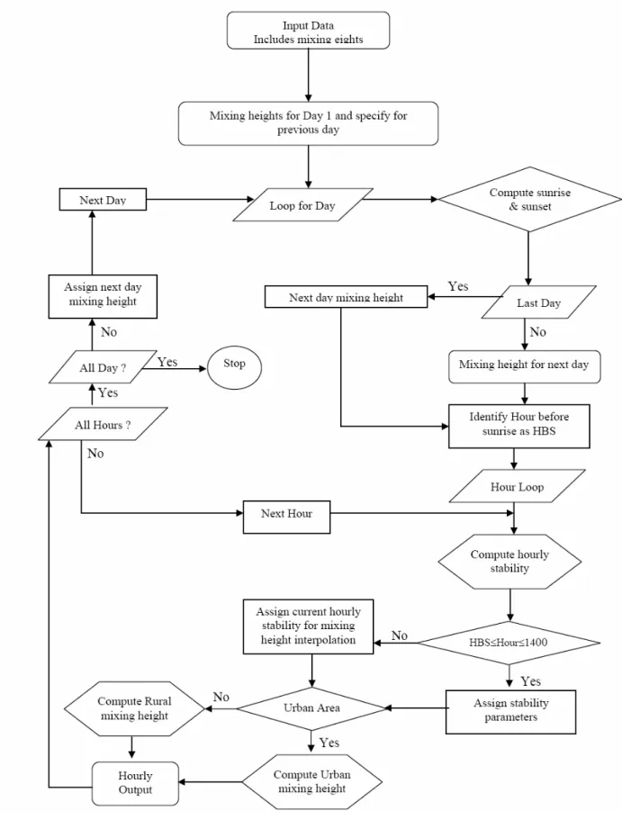
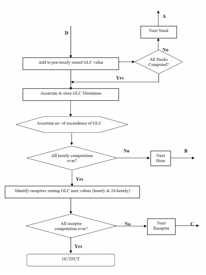
The overall computational program comprises two modules written in efficient code using 'C' language [12]. Each module is independent and generates information to be used by other modules for achieving accurate computation. The first module is called "preprocessing module" that is developed for appropriate processing of basic environmental data and details of it is shown in Figure 1 as a flow chart.
It aims at preparing a data file of hourly meteorological parameters to be used in the second module for the computation of ground level concentration (GLC). It also creates a data file of daily temporal data of sunrise and sunset for computation regime that finally generates the output.
5. Results and discussion
Some case studies are analyzed in order to demonstrate the features of the computational algorithm developed. Four major distinct cases are elucidated as given below:
Case 1: Single industrial operation [2×500 MW power plant]
Case 2: Single industrial operation [3×500 MW power plant]
Case 3: Single industrial operation [1×100 TPD Sponge Iron]
Case 3(a): Single industrial operation [1×100 TPD Sponge Iron] with Flue Gas Desulfurization (FGD) system having 80% SO2 removal efficiency
Case 4: Cumulative effect of the above three cases.
Case 4(a): Cumulative effect of Case 1, Case 2 and Case 3(a).
The co-ordinates of the three industrial establishments are different. These industrial units are located in rural environment that means these are not located in an industrial area. The pollutant under consideration is SO2, background concentration of which is 22 µg/m3. The dispersion study was carried out considering the winter season anticipating that results would yield worst scenario. And in that the decision taken with the help of such data on worst scenario would be more realistic for the design purpose as also for the purpose of policy making. It was planned to establish three units under consideration at that locality. Therefore, it is mandatory to carry out an Environmental Impact Assessment (EIA) for such industrial activities as per the EIA Notification of India [13] so as to maintain the background level of pollutant well within the permissible level. The area under question has been earmarked for further industrial development. Since the pollutant SO2 is deleterious and no stack emission standard has so far been fixed in India for its discharge from the stack for such industrial activities, its GLC value is necessary to be evaluated. Based on such predictive value, decision could be taken by the regulatory authority.
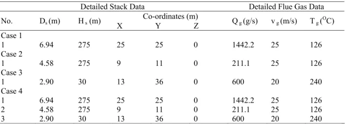
The details of the point sources are furnished in Table 1. The stack details and flue gas details are all presented in Table 2.
Table 1. Particulars of point sources
Parameters Case 1 Case 2 Case 3
Site Status Rural and Residential
Pollutant SO2
Background Value 22.0 µg/m3
Computation Period Winter 1995 – 1996
Area Covered 50 km × 50 km 50 km × 50 km 50 km × 50 km No. of Receptors 51×51
along X-Y co-ordinates
51×51
along X-Y co-ordinates
51×51
along X-Y co-ordinates
Table 2. Stack and flue gas details
Detailed Stack Data Detailed Flue Gas Data Co-ordinates (m)
No. Ds (m) H s (m)
X Y Z Q g (g/s) v g (m/s) T g ( O
C)
Case 1
1 6.94 275 25 25 0 1442.2 25 126
Case 2
1 4.58 275 9 11 0 211.1 25 126
Case 3
1 2.90 30 13 36 0 600 20 240
Case 4
1 6.94 275 25 25 0 1442.2 25 126
2 4.58 275 9 11 0 211.1 25 126
The meteorological data for the winter months of 1995 – 1996 was considered for evaluating the worst scenarios. The industrial are is located close to Durgapur at Barddhaman District located in the State of West Bengal. The GLC distribution pattern was evaluated on a rectangular area of 50 km × 50 km area having 51×51 receptors as square grids along X-Y co-ordinates. In fact, the EIA study conducted for the industrial operation as described in Case 1, 2, 3 and 3(a) as per the requirement of Indian guidelines has been envisaged here. The NAAQS [16] of India is furnished in Table 3 for assessing the 24 hourly maximum GLC values of SO2 obtainable for a specific case as to whether exceeded the permissible limit of the specific class. Thus the impacts of each of the three units in isolation as also the cumulative impact of the three units taken together are evaluated from the computational work.
Table 3. National Ambient Air Quality Standards (NAAQS) of India
Concentration in Ambient Air [µg/m3]
Pollutant Time Weighted
Average Industrial Area
Residential, Rural and other Areas
Sensitive Area
Annual Average* 80 60 15
Sulfur Dioxide (SO2)
24 Hours Average** 120 80 30
Annual Average* 80 60 15
Oxides of Nitrogen as NO2 24 Hours Average** 120 80 30
Annual Average* 360 140 70
Suspended Particulate Matter
24 Hours Average** 500 200 100
Annual Average* 120 60 50
Respirable Particulate Matter
(Size less than 10µm) 24 Hours Average** 150 100 75
* Annual Arithmetic mean of minimum 104 measurements in a year twice a week 24 hourly at uniform interval.
** 24 hourly/8 hourly values should be met 98% of the time in a year. However, 2% of the time, it may exceed but not on two consecutive days.
Note
1. National Ambient Air Quality Standard: The levels of air quality necessary with an adequate margin of safety, to protect the public health, vegetation and property.
2. Whenever and wherever two consecutive values exceed the limit specified above for the respective category, it would be considered adequate reason to institute regular/continuous monitoring and further investigations.
3. The State Government / State Board shall notify the sensitive and other areas in the respective states within a period of six months from the date of notification of National Ambient Air Quality Standards [Four parameters relevant to the present study are shown]
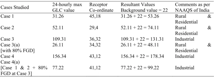
The detailed results of 24 hourly maximum GLC values are shown in Table 4. This table includes 24 hourly maximum predicted GLC values of SO2, respective receptor co-ordinates, resultant values and comments as per NAAQS of India.
It can be seen from the table that the 24 hourly maximum GLC values of SO2 for Case 1 and Case 2 would be 31.26 µg/m3 and 52.11 µg/m3 respectively. The respective resultant values were found to be 53.26 µg/m3 and 74.11 µg/m3 and were conformed to the value of Rural and Residential area specified in the NAAQS of India. Case 3 while yielded 24 hourly maximum GLC value of 109.31
GLC value would be 156.34 µg/m3 with the resultant value of 178.34 µg/m3. These values were well above the value of Industrial area stipulated in the NAAQS of India. Further, it was suggested to consider Case 3(a) in addition to Case 1 and Case 2 to predict the cumulative impact of SO2 emission and found that the 24 hourly maximum GLC value was 77.22 µg/m3 with the resultant value of 99.22
µg/m3. Though the absolute cumulative value of 77.22 µg/m3 was below the value stipulated for Rural and Residential area stipulated in the NAAQS of India, the resultant value of 99.22 µg/m3 was 25% higher than 80 µg/m3, the value stipulated for Rural and Residential area and is falling under Industrial area specified in the NAAQS of India. The location of the three industrial units and their 24 hourly maximum GLC values are shown in Figure 3 on a 50×50 grids covering an area of 50 km × 50 km. The cumulative impacts were also shown in the figure. The location of the power plant having capacity of 2×500 MW was considered Case 1 and its co-ordinate was fixed at (25 km, 25 km). Accordingly, the co-ordinates of other units were located. Figure 3 also described the receptor numbering system for the present study. This would help in understanding the receptor location with the specific Cartesian co-ordinate system.
Table 4. Maximum 24-hourly and 1-hourly GLC values in µg/m3
Cases Studied 24-hourly max GLC value
Receptor Co-ordinate
Resultant Values Background value = 22
Comments as per NAAQS of India
Case 1 31.26 45,18 31.26 + 22 = 53.26 Rural &
Residential
Case 2 52.11 29,4 52.11 + 22 = 74.11 Rural &
Residential Case 3 109.31 36,32 109.31 + 22 = 131.31 Industrial Case 3(a)
[with 80% FGD]
26.11 34,32 26.11 + 22 = 48.11 Rural & Residential Case 4 156.34 43,12 156.34 + 22 = 178.34 Industrial Case 4(a)
[Case 1 & 2 + 80% FGD at Case 3]
77.22 41,12 77.22 + 22 = 99.22 Industrial
0 5 10 15 20 25 30 35 40 45 50 0 5 10 15 20 25 30 35 40 45 50 Receptor Identification
Each Quadrant comprises 25×25 Grids = 625 Receptors 1st Quadrant: 1 to 625 Receptors
2nd Quadrant: 626 to 1250 Receptors 3rd Quadrant: 1251 to 1875 Receptors 4th Quadrant: 1876 to 2500 Receptors C4
C3(a)
Legend
Symbol Description of Point Source S1: 2×500 MW Power Plant S2: 3×500 MW Power Plant S3: 1×100 TPD Sponge Iron Plant C1: GLC Max due to S1 C2: GLC Max due to S2 C3: GLC Max due to S3
C3(a): GLC Max due to S3 [with 80% FGD] C4: Cumulative GLC Max
C4(a): Cumulative GLC Max [Case 1 & 2 + 80% FGD on C3]
C4(a) C2 C1 C3 S3 S2 S1 C ros s w in d D ist ance, y , [ × 1 000] m
Downwind Distance, x, [×1000] m
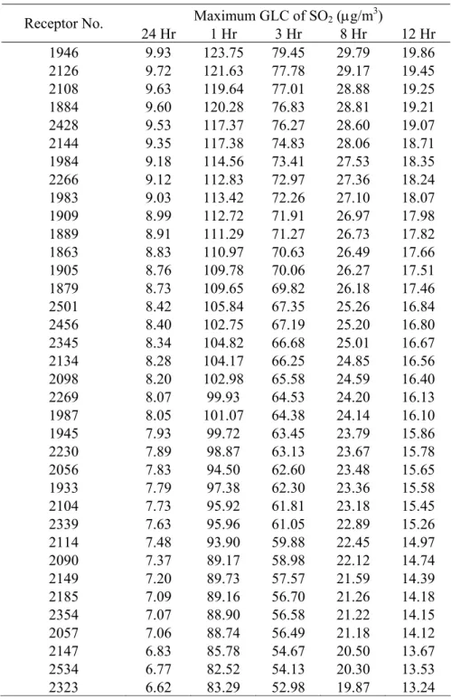
The prediction was processed to compute maximum GLC values for 24 hour, 1 hour, 3 hour, 8 hour and 12 hour averaging periods. Maximum GLC values were then arranged in descending order with respect to 24-houriy averaging periods. Such detailed break up of maximum GLC values obtained through the rigorous computational work for Case 1 as a typical case has been detailed in Table 5 for our improved understanding.
Table 5. Case study 1: maximum 24 hourly GLC of SO2
Maximum GLC of SO2 (µg/m3) Receptor No.
24 Hr 1 Hr 3 Hr 8 Hr 12 Hr
1946 9.93 123.75 79.45 29.79 19.86
2126 9.72 121.63 77.78 29.17 19.45
2108 9.63 119.64 77.01 28.88 19.25
1884 9.60 120.28 76.83 28.81 19.21
2428 9.53 117.37 76.27 28.60 19.07
2144 9.35 117.38 74.83 28.06 18.71
1984 9.18 114.56 73.41 27.53 18.35
2266 9.12 112.83 72.97 27.36 18.24
1983 9.03 113.42 72.26 27.10 18.07
1909 8.99 112.72 71.91 26.97 17.98
1889 8.91 111.29 71.27 26.73 17.82
1863 8.83 110.97 70.63 26.49 17.66
1905 8.76 109.78 70.06 26.27 17.51
1879 8.73 109.65 69.82 26.18 17.46
2501 8.42 105.84 67.35 25.26 16.84
2456 8.40 102.75 67.19 25.20 16.80
2345 8.34 104.82 66.68 25.01 16.67
2134 8.28 104.17 66.25 24.85 16.56
2098 8.20 102.98 65.58 24.59 16.40
2269 8.07 99.93 64.53 24.20 16.13
1987 8.05 101.07 64.38 24.14 16.10
1945 7.93 99.72 63.45 23.79 15.86
2230 7.89 98.87 63.13 23.67 15.78
2056 7.83 94.50 62.60 23.48 15.65
1933 7.79 97.38 62.30 23.36 15.58
2104 7.73 95.92 61.81 23.18 15.45
2339 7.63 95.96 61.05 22.89 15.26
2114 7.48 93.90 59.88 22.45 14.97
2090 7.37 89.17 58.98 22.12 14.74
2149 7.20 89.73 57.57 21.59 14.39
2185 7.09 89.16 56.70 21.26 14.18
2354 7.07 88.90 56.58 21.22 14.15
2057 7.06 88.74 56.49 21.18 14.12
2147 6.83 85.78 54.67 20.50 13.67
2534 6.77 82.52 54.13 20.30 13.53
6. Recommendations
The computational results clearly revealed that the 24 hourly maximum GLC values under worst scenario for Case 1 and Case 2 in isolation would not affect the air quality in respect of SO2 discharge from the stacks in the surrounding area. In contrast, Case 3 affect the air quality adversely but suggesting FGD system having 80 % SO2 removal efficiency drastically reduced the 24 hourly maximum GLC value. The cumulative impact of Cases 1, 2 and 3 showed adverse predicted value while Case 3(a) that assumes FGD system having 80 % SO2 removal efficiency resulted in the predicted value of 24 hourly maximum GLC of SO2 favorable. It is therefore, recommended that these three industrial units would be permitted to be established with the condition that the sponge iron plant should have a FGD system that is at least 80 % efficient in removing SO2 from the waste gas stream of the sponge iron plant. Since Gaussian dispersion modeling does not take into account any chemical reaction, the model reported in this article can be squarely applicable for similar other pollutants like particulate matter, NOx etc. emitted in association with the SO2 from stacks.
7. Conclusions
Gaussian dispersion modeling necessitates the knowledge of stability of the atmosphere, mixing height, plume rise, dispersion parameters etc. In India, the methods of obtaining values of these parameters are all taken from available literatures and to ascertain their applicability in Indian context has not gained any attention. Validation of these formulations is thus necessary through extensive monitoring of various parameters. It is thus aimed in this article to propose computational algorithm in order to validate these formulations through extensive monitoring of various parameters. In the process, various strategies of pollution control are elucidated so that the most appropriate combination of industrial activities would be chosen for arriving at an environment friendly air quality. An assessment of suitability of a site for setting up of new industry would thus be possible. However, the full strength of the model proposed can only be exploited if sufficient information on environmental parameters is available for reasonable period of time. In view of the fact of sparse Indian mixing height data, efforts are needed to generate mixing height data.
Broadly four different cases were analyzed based on worst scenario. Results obtained through prediction were compared with NAAQS of India. One specific case found to overshoot the ambient air quality adversely in respect of SO2 and was therefore, suggested to install a FGD system with at least 80 % SO2 removal efficiency. With this recommendation, the cumulative prediction yielded a very conservative resultant value of 24 hourly maximum GLC of SO2 as against a value that exceeded well above the stipulated value without considering the FGD system. The computational algorithm developed can be gainfully utilized for the purpose of EIA analysis in Indian condition.
Acknowledgements
The author thankfully acknowledges the assistance provided by M/s Development Consultant Ltd., Kolkata, India, for the research work during 1996 – 1998.
References
[1] Mukherjee P., Viswanathan S., Choon L. C. Modeling mobile source emissions in presence of stationary sources. J of Haz. Mat. 2000, 76(1), 23–37.
[2] Dabberdt W. F., Miller E. Uncertainty, ensembles and air quality dispersion modeling: applications and challenges. Atm. Env. 2000, 34(27), 4667–4673.
[3] Jiang W., Hu F., Wang W. A non-hydrostatic dispersion modeling system and its application to air pollution assessments over coastal complex terrain. J of Wind Eng. and Ind.l Aerodyn. 2000, 87(1), 15–43.
[4] Borrego C., Tchepel O., Costa A. M., Amorim J. H., Miranda A. I. Emission and dispersion modelling of Lisbon air quality at local scale. Atm. Env. 2003, 37(37), 5197–5205.
[5] Rama Krishna T.V.B.P.S., Reddy M.K., Reddy R.C., Singh R.N. Impact of an industrial complex on the ambient air quality: Case study using a dispersion model. Atm. Env. 2005, 39(29), 5395– 5407.
[7] Baroutian S., Mohebbi A., Goharrizi A. S. Measuring and modeling particulate dispersion: A case study of Kerman Cement Plant. J of Haz. Mat. 2006, 136(3), 468–474.
[8] Liu G., Fu E., Wang Y., Zhang K., Han B., Arrowsmith C. A Framework of Environmental Modelling and Information Sharing for Urban Air Pollution Control and Management. J. of China Univ. of Min. and Tech. 2007, 17(2), 172–178.
[9] Carmichael G. R., Sandu A., Chai T., Daescu D. N., Constantinescu E. M., Tang Y. Predicting air quality: Improvements through advanced methods to integrate models and measurements. J. of Comp. Phy. 2008, 227(7), 3540–3571.
[10] Elkamel A., Fatehifar E., Taheri M., Al-Rashidi M.S., Lohi A. A heuristic optimization approach for Air Quality Monitoring Network design with the simultaneous consideration of multiple pollutants. J. of Env. Manag. 2008, 88(3), 507–516.
[11] Ainslie B., Jackson P.L. The use of an atmospheric dispersion model to determine influence regions in the Prince George, B.C. airshed from the burning of open wood waste piles. J.of Env. Manag. 2009, 90(8), 2393–2401.
[12] DCL, Dispersion of Pollutants in Air Emitted from Multiple Sources: Volume – I. Report prepared under the aegis of Ministry of Power, Government of India under Research Scheme on Power. September 1996. Development Consultants Limited. Kolkata.
[13] MoEF. Environment Impact Assessment Notification [S.O.1533, dated 14.09.2006], Ministry of Environment and Forests. Government of India. New Delhi. 2006.
[14] CPCB. Guidelines for Air Pollutants Dispersion Modelling from Point Sources. PCI-II Division, Central Pollution Control Board, East Arjun Nagar, New Delhi. 1995.
[15] Bierly E.W., Hewson E.W. Some restrictive meteorological conditions to be considered in the design of stacks. J. of Appl. Meteorol. 1962, 1(3), 383–390.
[16] MoEF. Air (Prevention & Control of Pollution) Act, S.O. 384(E), dated April 11, 1994. Central Pollution Control Board, Ministry of Environment of and Forests, Government of India. New Delhi. 1994.
Amitava Bandyopadhyay:
9 B.Tech. Chemical Technology. University of Calcutta, India. 1988, First Class First.
9 M.Tech. Chemical Engineering. Indian Institute of Technology, Kharagpur, India. 1990.
9 Ph.D. Chemical Engineering. Indian Institute of Technology, Kharagpur, India. 1996.
Major fields of study: Air Quality Modeling, Air Pollution Control, CO2 Capture, Wet Scrubber Modeling,
Advances Waste Water Treatment, Gas-Liquid Mass Transfer Operations, Waste Management especially Electronics Waste and Hazardous Wastes. Risk and Consequence Analyses.
He has published 29 articles in peered reviewed International Journals. At national level he has so far published 30 articles. Before joining as a Faculty Member in the Department of Chemical Engineering at the University of Calcutta he has served Indian Regulatory Agency for a period of more than 10 years in a very senior position dealing with implementation of various Environmental Rules and Regulations. Legion of technical reports prepared by him on the premise of Indian regulatory regimes on the abatement of industrial of pollution have been used with great success in the country, for instance, the National Environmental Standards on its revision on Indian Petroleum Oil Refinery includes the effluent discharge parameters after careful consideration of his action taken report on an Indian Petroleum Oil Refinery. He was a state representative for the Development of Emission Standards for Indian Petrochemical Industries under the World Bank funded Project. He has visited Japan and the USA and visited a large number of industries.
Dr. Bandyopadhyay has received several laurels for his excellent research works. He has organized several Symposia, Workshops etc as also chaired a number of technical sessions of national/international events on Environmental Sciences & Engineering. He is carrying out many projects related to environmental pollution control. Dr. Bandyopadhyay is involved as a key person in the CO2
Capture Projects from Coal Fired Thermal Power Plants in the State of West Bengal. He is a Member of the Editorial Board of Journal of Water Resource & Protection of Scientific Research Publication, and a Member of the Editorial Advisory Board of International Journal of Environmental Science & Technology of Iranian Society of Environmentalists. Dr. Bandyopadhyay is a Life Member of several professional bodies like, The Institution of Engineers (India); Indian Institution of Chemical Engineers; Institution of Public Health Engineers, India; Oil Technologists Association of India: Coal Ash Institute of India; Air Pollution Control Association of India; Indian Water Works Association; Indian Association for Environmental Management; Indian Science Congress Association.