INTERPOLATION OF AIR QUALITY MONITORING DATA IN AN URBAN SENSITIVE AREA: THE OPORTOASPRELA CASE

6

INTERPOLATION OF AIR QUALITY MONITORING

DATA IN AN URBAN SENSITIVE AREA:

THE OPORTO/ASPRELA CASE

Tânia Fontes

Doctoral Student of Environmental Sciences CIAGEB, Faculty of Science and Technology University Fernando Pessoa, Porto, Portugal

tania@ufp.edu.pt

Nelson Barros

Associate Professor

CIAGEB, Faculty of Science and Technology University Fernando Pessoa, Porto, Portugal

nelson@ufp.edu.pt

ISSN: 1646-0499

7

ABSTRACT

At urban level, the representativity of air quality measurements is low which requires a den-se measurement network and/or the uden-se of complementary techniques for the air quality evaluation. Based on data from an air quality campaign and from the national air quality network, this article explores two interpolation methods in order to select the best for the air quality concentration field estimation in a sensitive urban area. The preliminary analysis indicates that the IDW is the best air quality interpolation method for the study domain.

KEYWORDS

air pollution, spatial distribution, interpolation.

RESUMO

A nível urbano, a representatividade das medições da qualidade do ar é baixa, exigindo uma densa rede de medição e/ou recurso a técnicas complementares para a avaliação da qualidade do ar. Baseado em dados de uma campanha e da rede nacional de qualidade do ar, este artigo explora dois métodos de interpolação para seleccionar o melhor método de estimativa da qualidade do ar numa área urbana sensível. A análise preliminar indica que o IDW é o melhor método de interpolação para o domínio de estudo.

PALAVRAS-CHAVE

poluição do ar, distribuição espacial, interpolação.

8

1.

INTRODUCTION

In most urban areas, as Oporto, the road transports are one of the main source of ambient air

concentrations of pollutants such as nitrogen oxides (NO2), carbon monoxide (CO), benzene

(C6H6), and particles (Alpopi; Keuken et al.). In order to monitoring this problem, have been

generated maps of concentrations by mean interpolating and extrapolating methods and in the recent years, urban air quality monitoring and forecast has become an important issue for many environmental protection agencies around the world (Horálek et al.).

Spatial prediction techniques, also known as spatial interpolation techniques, differ from classical modelling approaches in that they incorporate information on the geographic po-sition of the sample data points (Cressie). The interpolation is the procedure of predicting unknown values using the known values at neighbouring locations which may be regularly or irregularly spaced. The values derived in this way are not necessarily the true value; they are a mathematical “best guess” based on the known values (Aranoff ). Thus this method is necessary when the ground truth data do not cover the wholly domain. Demers, classify the interpolation methods on linear and non linear.

Usually the interpolation methods use the weighted average of nearby data to calculate the estimates. The weights could be assigned according to deterministic or statistical criteria. The quality of the interpolation results depends on the accuracy, number, and distribution of the known points used in the calculation and on how well the mathematical function correctly models the phenomenon (Aranoff ). Also, the pollutants are governed by different mechanism, of acting on a different spatial scale: regional and local effects. Fluctuations in the concentration pattern are mainly driven by meteorological phenomena; however air pollution can have a distinct local character due to local emission sources and their tem-poral variability. In the dense urbanized region of Asprela in Oporto, the study domain, the latter effects are significant. This is a sensitive area with several universities and two hospitals, with high traffic density and mobility problems, however does not have any air quality site of the national network.

Among statistical methods, geostatistical kriging-based techniques, including simple and ordinary kriging, universal kriging and simple cokriging have been used for spatial analy-sis. In the deterministic interpolation methods, inverse distance weighting method and its modifications are the most often applied. Kriging and IDW are the most commonly used methods in air quality (Wong et al.; Horálek; Mesquita; Sánchez). Both methods estimate values at unsampled locations based on the measurements at surrounding locations with certain assigned weights for each measurements. However, while kriging requires the pre-liminary modelling step of a variance-distance relationship, IDW does not require this step. Many studies have compared IDW and kriging, and generally the performance of kriging was generally better (Wong et al.).

9

This work was performed over the first of two seasonal campaigns (winter and summer) planned for Asprela domain.

The outline of this paper is as follows: in Section 2 methodology is described in detail and in Sec-tion 3 and 4 model results are discussed and validated. A conclusion is presented in SecSec-tion 5.

2.

METHODOLOGY

For the present study was used the C6H6 and NO2 atmospheric concentration in the Asprela

domain, two pollutants considered good markers of traffic pollution, the most important emission source at the domain. These pollutants were measured in the scope of the CIVITAS--ELAN project (TREN/FP7TR/218954 - ELAN).

Statistical analyses were done in two stages. First geostatistical analysis was performed and then the distribution of data was described using conventional statistics such as mean, ma-ximum, minimum and standard deviation (SD). In this second step results were compared also with the annual limit value for the protection of human health defined in the Directive

2008/50/CE (5 µg.m-3 _{for C}

6H6 and 40 µg.m-3 for NO2). Although these limits are linked to

annual averages and the results are to a short campaign (three weeks), this approach re-presents a good indicator of the potential impact on human health of air quality in Asprela (study domain).

Regarding to the first step, firstly was define the number of observation points needed for a correct spatial representation of atmospheric concentrations field in the domain. To do this was used a statistic approach based on an estimate made by a numerical dispersion model.

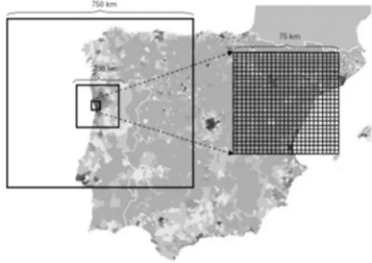
Due its ability to reproduce mesoscale atmospheric circulations and photochemical produc-tion, the application to long data series, as well as, its speed of data processing the air quality modelling was performed using the TAPM model (Hurley). The model was applied using a three level nesting technique with 25 x 25 points, centred on the city of Oporto (41 ° 9’34, 94’’N, 8 ° 37’19, 32’’W) and 25 vertical grid levels, between 10 and 8 000 meters. The larger grid use cells of 30 km x 30 km, the intermediate grid, cells of 10 km x 10 km and the finer grid, cells of 3 km x 3 km (Figure 1). The synoptic forcing was done based on the ECMWF data to the year of 2006, a year considered a good approximation to the climatic normal of

the study region (Fontes). The simulation of air quality was made using CO and NO2 UNECE

emissions (Boavida et al.) for the finer grid. Because the UNECE emission inventory does not

include C6H6 emissions the TAPM model was used to simulate, as a tracer of C6H6, the CO

concentrations. Thus, two types of air quality simulations were done, one in non-reactive

mode to CO concentrations, and another in reactive mode for NO₂. In the reactive mode

simulation was considered a value of reactivity pattern of VOC emissions (Rsmog) of 0.0067

(Hurley et al.). Additionally, in order to get a refinement of the concentration field over the study domain, the output grid was processed to a sub-grid with cells of 300 m x 300 m. The simulation was performed between 19/11 and 16/12, which corresponds to the period of the field winter campaign.

Using the estimate concentrations over Asprela (Figure 2), was calculated an CO average

concentration of 241.86 ± 13.80 µg.m-3 _{and a NO}

2 concentration of 18.43 ± 0.51 µg.m-3.

10

points for each pollutant, considering that the confidence level (LC) have a significance level of 5% of the mean value (Eq. 1).

Figure 1. Meteorological domains considered in the air quality simulation using TAPM model in MAO.

𝐿𝐿𝐿𝐿𝐿𝐿𝐿𝐿

=

𝑅𝑅𝑅𝑅

√𝑛𝑛𝑛𝑛

𝑡𝑡𝑡𝑡

0.975

<=>

𝑛𝑛𝑛𝑛

=

�

𝑅𝑅𝑅𝑅

𝐿𝐿𝐿𝐿𝐿𝐿𝐿𝐿 𝑡𝑡𝑡𝑡

0.975

�

2

(Eq. 1)

This approach resulted in an estimate of about 6 observation points to CO and 2 to NO2

required to a representative description of the study domain.

11

ii)

Figure 2. Air concentrations (µg.m-3_{) estimated by TAPM model in the Asprela domain: i) CO; ii) and NO} 2.

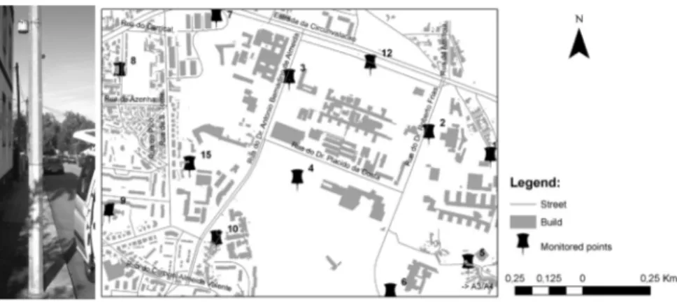
Based on these results, the field campaign was designed and, as presented previously, took place between 19/11/2009 and 16/12/2009, using a diffusive sampler’s technique (PASSAM). In order to control eventual deviations and diffusive samplers lost due vandalism, was used 12 observation points. The diffusive samplers were placed at 3 m high and evenly distri-buted on the domain (Figure 3). Additionally, and in order to monitoring the background concentration, measurements were also done at the top of four buildings of the city (40-50 m high): Antas tower, Burgos building, JN building and CMP building. In these locals were used replicas in order to control eventual deviations. In this campaign and due to vandalism the point number 4 of C6H6 was lost.

Figure 3. Location of the diffusive measurements in the Asprela domain.

To estimate the spatial distribution of C6H6 and NO2 during the winter campaign at

12

The IDW is a method often used to interpolate data from air quality, given its simplicity (Brigs et al.; Keuken et al.; Lindley and Walch). To predict a value for any unmeasured location, this method uses the measured values surrounding the prediction location. Closest values have more influence on the predicted value than those farther away, hence the name inverse distance weighted. The surface calculated depends on the selection of a power value and the neighbourhood search strategy. IDW is an exact interpolator, where the maximum and minimum values in the interpolated surface can only occur at sample points. The output surface is sensitive to clustering and the presence of outliers. IDW assumes that the surface is being driven by the local variation, which can be captured through the neighbourhood.

𝑓𝑓𝑓𝑓(𝑥𝑥𝑥𝑥,𝑖𝑖𝑖𝑖) =�∑ 𝑤𝑤𝑤𝑤(𝑈𝑈𝑈𝑈𝑖𝑖𝑖𝑖)𝑧𝑧𝑧𝑧𝑖𝑖𝑖𝑖

𝑛𝑛𝑛𝑛 𝑖𝑖𝑖𝑖=1

∑𝑛𝑛𝑛𝑛_{𝑖𝑖𝑖𝑖=1}𝑤𝑤𝑤𝑤(𝑈𝑈𝑈𝑈_{𝑖𝑖𝑖𝑖})�,𝑖𝑖𝑖𝑖= 1,2, … ,𝑛𝑛𝑛𝑛 (Eq. 2) Where zi is a observed value i; di is the distance between the estimated point and the obser-ved point i; w(di) = 1/(di)p is the ponderation of the observation i; and p is the power function.

The IDW predictions were performed varying the number of power (0.5 and 3) and using different radiuses and neighbours.

The kriging method is similar to the IDW for considering the measured values in the neigh-bourhood for predict the concentrations in an unmeasured location. In ordinary kriging the weights depends on the model fitted to the measurement points of the local distance esti-mate, and the spatial relationships between the measured values around the local forecast (Johnston et al.). Ordinary kriging assumes the model:

𝑍𝑍𝑍𝑍(𝑠𝑠𝑠𝑠) =𝜇𝜇𝜇𝜇+𝜀𝜀𝜀𝜀(𝑠𝑠𝑠𝑠) (Eq. 3)

Where µ is an unknown constant.

The performance of each evaluation technique was assessed comparing the deviation of estimates using the cross-validation method. To use this technique, was excluded a point and then apply the model to estimate the concentrations in this removed point. Therefore, the comparison of the performance between the different interpolation techniques was achieved using the average error (ME)(Eq. 4), the Mean Absolute Error (MAE) (Eq. 5), the Root

Mean Squared Error (RMSE) (Eq. 6) and de Normalized Root Mean Squared Error (NRMSE) (Eq.

7), and the coefficient of determination (R2_{) (Eq. 8) (Mesquita):}

𝑀𝑀𝑀𝑀𝑀𝑀𝑀𝑀=1

𝑛𝑛𝑛𝑛 � 𝑀𝑀𝑀𝑀𝑖𝑖𝑖𝑖− 𝑂𝑂𝑂𝑂𝑖𝑖𝑖𝑖 𝑛𝑛𝑛𝑛

𝑖𝑖𝑖𝑖=1

(Eq. 4)

𝑀𝑀𝑀𝑀𝑀𝑀𝑀𝑀𝑀𝑀𝑀𝑀=1

𝑛𝑛𝑛𝑛 �|𝑀𝑀𝑀𝑀𝑖𝑖𝑖𝑖− 𝑂𝑂𝑂𝑂𝑖𝑖𝑖𝑖| 𝑛𝑛𝑛𝑛

𝑖𝑖𝑖𝑖=1

(Eq. 5)

𝑅𝑅𝑅𝑅𝑀𝑀𝑀𝑀𝑅𝑅𝑅𝑅𝑀𝑀𝑀𝑀=�1

𝑛𝑛𝑛𝑛 �(𝑀𝑀𝑀𝑀𝑖𝑖𝑖𝑖− 𝑂𝑂𝑂𝑂𝑖𝑖𝑖𝑖)2 𝑛𝑛𝑛𝑛

𝑖𝑖𝑖𝑖=1

13

𝑁𝑁𝑁𝑁𝑅𝑅𝑅𝑅𝑀𝑀𝑀𝑀𝑅𝑅𝑅𝑅𝑀𝑀𝑀𝑀=𝑅𝑅𝑅𝑅𝑀𝑀𝑀𝑀𝑅𝑅𝑅𝑅𝑀𝑀𝑀𝑀

𝑂𝑂𝑂𝑂�𝑖𝑖𝑖𝑖 (Eq. 7)

𝑅𝑅𝑅𝑅2_{= 1−}∑ (𝑂𝑂𝑂𝑂𝑖𝑖𝑖𝑖− 𝑀𝑀𝑀𝑀𝑖𝑖𝑖𝑖) 2 𝑛𝑛𝑛𝑛

𝑖𝑖𝑖𝑖=1

∑𝑛𝑛𝑛𝑛 (𝑂𝑂𝑂𝑂_{𝑖𝑖𝑖𝑖}− 𝑂𝑂𝑂𝑂�_{𝑖𝑖𝑖𝑖})2 𝑖𝑖𝑖𝑖=1

(Eq. 8)

Where: E = Estimated value; O = Observed value; n = Number of cases; Ō = Mean of

ob-served values.

All of these parameters have to be equal or close to zero, except the R2 _{where the optimal}

value is 1.

To verify if the selected map can be considered from the legal point of view, was also calcu-lated, the value of uncertainty according to Directive 2008/50/EC:

𝑈𝑈𝑈𝑈𝑛𝑛𝑛𝑛𝑈𝑈𝑈𝑈𝑈𝑈𝑈𝑈𝑈𝑈𝑈𝑈𝑡𝑡𝑡𝑡𝑈𝑈𝑈𝑈𝑖𝑖𝑖𝑖𝑛𝑛𝑛𝑛𝑡𝑡𝑡𝑡𝑖𝑖𝑖𝑖=𝑂𝑂𝑂𝑂𝑂𝑂𝑂𝑂𝑠𝑠𝑠𝑠𝑈𝑈𝑈𝑈𝑈𝑈𝑈𝑈𝑂𝑂𝑂𝑂𝑈𝑈𝑈𝑈𝑈𝑈𝑈𝑈𝑂𝑂𝑂𝑂𝑈𝑈𝑈𝑈𝑣𝑣𝑣𝑣𝑣𝑣𝑣𝑣𝑈𝑈𝑈𝑈 − 𝑀𝑀𝑀𝑀𝑀𝑀𝑀𝑀𝑈𝑈𝑈𝑈𝑈𝑈𝑈𝑈𝑣𝑣𝑣𝑣𝑣𝑣𝑣𝑣𝑈𝑈𝑈𝑈𝑈𝑈𝑈𝑈𝑂𝑂𝑂𝑂𝑈𝑈𝑈𝑈𝑣𝑣𝑣𝑣𝑣𝑣𝑣𝑣𝑈𝑈𝑈𝑈

𝐿𝐿𝐿𝐿𝑖𝑖𝑖𝑖𝐿𝐿𝐿𝐿𝑖𝑖𝑖𝑖𝑡𝑡𝑡𝑡𝑂𝑂𝑂𝑂𝑈𝑈𝑈𝑈𝑣𝑣𝑣𝑣𝑣𝑣𝑣𝑣𝑈𝑈𝑈𝑈 (Eq. 9)

The results were compared with the uncertainty of estimation, for both pollutants, defined

by the Directive 2008/50/EC, 100% to C6H6 and 75% to NO2.

3.

RESULTS AND DISCUSSION

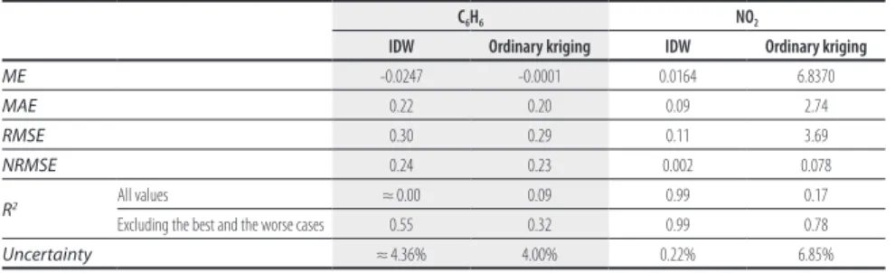
The Table 1 present the results of statistical analysis using cross-validation to the best inter-polation map, by pollutant and interinter-polation method, and the specifications are presented on Table 2. The comparison between the two methods of spatial distribution, IDW and

or-dinary kriging, shows that oror-dinary kriging is the best method to simulate the C6H6 but the

differences to the IDW method are small. In the case of the NO2 concentrations the IDW

gives better results. This fact may be related with different pattern of field concentrations for the study pollutants (different emission and reactivity pattern) and/or forced by the lack of one of the C6H6 control points (due to vandalism).

Table 1. Results of statistical analysis using cross-validation.

C6H6 NO2

IDW Ordinary kriging IDW Ordinary kriging

ME -0.0247 -0.0001 0.0164 6.8370

MAE 0.22 0.20 0.09 2.74

RMSE 0.30 0.29 0.11 3.69

NRMSE 0.24 0.23 0.002 0.078

R2 All values ≈ 0.00 0.09 0.99 0.17

Excluding the best and the worse cases 0.55 0.32 0.99 0.78

14

Table 2. Selected specifications by pollutant and method.

C6H6 NO2

IDW Ordinary kriging IDW Ordinary kriging

Specifications IDW

Output 5 - 5

-Power 3 - 1

-Search radius Variable - Variable

-Ordinary kriging

Method - Spherical - Gaussian

Lag size - 500 - 500

Major range - 1000 - 1000

Partial still - 15 - 15

Nugget - 30 - 30

Radius number of points: 6 12 16 12

In Figure 4 and 5 can be seen the two best maps resulting from different simulations for C6H6

and NO2 respectively using the IDW method and ordinary kriging.

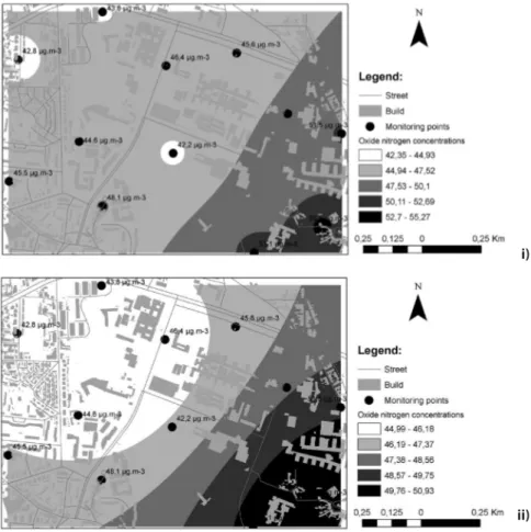
Although the C6H6 map does not presents hotspots the NO2 map shows some. This is the

case of sample 4 where the concentrations are less than to their neighbours (Figure 5). To this situation the IDW method can pick up these fluctuations better than ordinary kriging method. Although all domain is characterized by the presence of roads and car parking’s, this critical point (sample 4) was placed in an area surrounding by vegetation and a sports

park with low direct emission of pollutants. Due the vandalism the C6H6 concentrations in

this point were lost, but the recorded of NO2 concentrations confirm that this is an area with

less pollution. This fact can be decisive to show, in future campaigns, that IDW method may be the best interpolated method to the Asprela domain.

15

ii)

Figure 4. Average C6H6 concentrations (µg.m-3) in the Asprela domain during 19/11/-16/12/2009 using different

inter-polation methods: i) IDW, ii) Ordinary kriging.

i)

ii)

Figure 5. Average NO2 concentrations (µg.m-3) in the Asprela domain during 19/11/-16/12/2009 using different

16

Once validated and selected the best map for each pollutant, in the next chapter takes place the spatial analysis of the results.

4.

DATA ANALYSIS

To 3 m height, the observed average concentrations are 1.25 ± 0.23 µg.m-3 _{of C}

6H6 and

47.22 ± 4.18 µg.m-3 _{of NO}

2. For the two pollutants the minimum values are recorded close

the “Estrada da Circunvalação” and the maximum values are recorded in the south close the A3/A4 motorway where the volume of traffic increases and traffic speed decrease causing an emissions increase. The background average concentrations (observations in the tops of buildings) are 1.02 ± 0.11 µg.m-3 _{to C}

6H6 and 34.86 ± 1.45 µg.m-3 to NO2, 18% and 26% lower

than the average values recorded at 3 m respectively.

The uncertainty of the estimates for both pollutants is below the limits defined in Directive 2008/50/EC, 100% for C6H6 and 75% for NO2 (Table 1). Thus, these maps are representative of

the study area and are a good indicative tool to evaluate the results from the legal point of

view. The comparison of C6H6 results with the human health protection value of 5 µg.m-3

de-fined by the Directive 2008/50/EC shows that, during the period of study, in all monitoring

points, the C6H6 concentrations are lower than this limit value. Even considering the 23.0%

of uncertainty of the C6H6 measurement method (PASSAM) the measured concentrations

never exceed the average annual limit value for human health protection. On the other

hand, the average NO2 concentrations are in the whole study domain higher than the

aver-age annual limit value for human health protection defined by the Directive 2008/50/EC (40

µg.m-3_{). However, considering the 18.7% of uncertainty of measurement method (PASSAM)}

for NO2, 25% of these control points may not exceed the mentioned limit value.

4.

CONCLUSIONS

The used methods of spatial analysis in this study not allow the definition of an optimal inter-polation method for the winter campaign over the Asprela area. However the analysis indica-tes that, in general, the IDW method should be the best method to the study domain. In order to confirm this, other tests have to be done for other periods and pollutants. On the other hand, other methods such as ordinary cokriging or multiple linear regressions, using auxiliary variables to adjust the spatial interpolation, could be tested in order to minimize errors.

The results for this winter campaign show that, when compared with the Directive 2008/50/

EC average annual limit values for the human health protection, the C6H6 concentrations are

very low, while the NO2 concentrations presents some values above the that limit. Even

con-sidering the uncertainties of the measurement methods, the C6H6 recorded concentrations

are never above the annual average limit value for human health protection. Nevertheless,

the NO2 recorded concentrations are above of the annual average limit value for human

17

ACKNOWLEDGEMENTS

To Fundação para a Ciência e Tecnologia (FCT) for grant support to Tânia Fontes (Ref. SFRH/ BD/19027/2004). To European Union for funding the CIVITAS-ELAN project: Mobilising citi-zens for vital cities Ljubljana - Gent - Zagreb - Brno – Oporto (TREN/FP7TR/218954(ELAN)).

BIBLIOGRAPHY

Alpopi, C., and S. E. Colesca. “Urban Air Quality, a Comparative Study of Major European Capi-tals.” Theoretical and Empirical Researches in Urban Management 6.15 (2010): 92-107.

Aranoff, S. Geographic Information Systems: A Management Perspective. Ottawa, Canada: WDL Publications, 1995.

Brigs, D. J., et al. Air Pollution Modelling for Support to Policy on Health and Environmental Risks in Europe. Final Report Section 6. London: Imperial College, 2005.

Boavida, F., et al. Alocação espacial de emissões em 2005. Lisboa: Agência Portuguesa do Am-biente, 2008.

Cressie, N. A. Statistics for Spatial Data Revised Edition. New York: John Wiley & Sons Inc., 1993.

Demers, M. N. Fundamentals of Geographic Information Systems. New York: John Wiley & Sons. Inc., 2005.

Directive number 50 of 2008, Official Journal of 11 June 2008, L 152, pages 1-42 (Defines the Ambient Air Quality Guidelines to Avoid, Prevent or Reduce Harmful Effects on Human Health and the Environment).

Fontes, T. Impacte da qualidade do ar na saúde pública: o caso da cidade do Porto. PhD Diss. U Aveiro, 2010.

Johnston, Kevin, et al. Using ArcGIS Geostatistical Analyst: GIS by ESRI. Redlands, CA: Environ-mental Systems Research Institute, 2001.

Keuken, M., et al. “Health Effects of Transport-Related Air Pollution, Contribution of Traf-fic to Levels of Ambient Air Pollution in Europe.” Biblioteca Virtual de Desarollo Sostenible y Salud Ambiental. 2004. Internet. 16 Apr. 2010. <http://www.bvsde.paho.org/bvsacd/cd63/ e86650/cap2.pdf>.

Horálek, J., et al. “Interpolation and Assimilation Methods for European Scale Air Quality As-sessment and Mapping - Part II: Development and Testing New Methodologies ETC/ACC Technical Paper 2005/8.” European Topic Centre on Air and Climate Change. 14 Feb. 2006. Internet. 16 Apr. 2010. <http://air-climate.eionet.europa.eu/reports/ETCACC_TechnPa-16 Apr. 2010. <http://air-climate.eionet.europa.eu/reports/ETCACC_TechnPa-per_2005_8_Spatial_AQ_Dev_Test_Part_II>.

18

Hurley, P., W. Physick, and A. Luhar. “TAPM – A Practical Approach to Prognostic Meteorologi-cal and Air Pollution Modelling.” Env. Modelling and Software .20 (2005): 737-52.

Lindley, S. J., and T. Walch, “Inter-Comparison of Interpolated Background Nitrogen Dioxide Concentrations Across Greater Manchester.” Atm Env 39.15 (2005): 2709-24.

Mesquita, S. Modelação da distribuição espacial da qualidade do ar em Lisboa Usando Sistemas de Informação Geográfica. Master thesis, U Nova de Lisboa, 2010.

PASSAM. 2010. Internet. 16 Apr. 2010 <http://www.passam.ch/>.

Sánchez, H. U. et al. “The Spatial-Temporal Distribution of the Atmospheric Polluting Agents During the Period 2000-2005 In the Urban Area of Guadalajara, Jalisco, Mexico.” J Hazardous Materials 165.1-3 (2009): 1128-41.