www.ann-geophys.net/29/965/2011/ doi:10.5194/angeo-29-965-2011
© Author(s) 2011. CC Attribution 3.0 License.
Annales
Geophysicae
Data derived NARMAX Dst model
R. J. Boynton1, M. A. Balikhin1, S. A. Billings1, A. S. Sharma2, and O. A. Amariutei3
1Department of Automatic Control and Systems Engineering, University of Sheffield, Sheffield, UK 2Department of Astronomy, University of Maryland, College Park, MD, USA
3Geophysical Research, Finnish Meteorological Institute, Helsinki, Finland
Received: 28 February 2011 – Revised: 17 May 2011 – Accepted: 18 May 2011 – Published: 1 June 2011
Abstract. The NARMAX OLS-ERR methodology is ap-plied to identify a mathematical model for the dynamics of the Dst index. The NARMAX OLS-ERR algorithm, which is widely used in the field of system identification, is able to identify a mathematical model for a wide class of non-linear systems using input and output data. Solar wind-magnetosphere coupling functions, derived from analytical or data based methods, are employed as the inputs to such models and the outputs are geomagnetic indices. The newly deduced coupling function,p1/2V4/3BTsin6(θ/2), has been implemented as an input to model the Dst dynamics. It was shown that the identified model has a very good forecasting ability, especially with the geomagnetic storms.
Keywords. Magnetospheric physics (Solar wind-magnetosphere interactions)
1 Introduction
The Earth’s magnetosphere is a complex nonlinear system that responds to solar wind. This complexity means that un-til now the derivation of a mathematical model from first principles have been unsuccessful. However, the magneto-sphere is a low-dimensional system (Sharma, 1995; Valdivia et al., 1996; Klimas et al., 1996) and therefore the robust machinery of a low-dimensional system identification tech-nique can be applied in the quest for a mathematical model of the magnetospheric dynamics. The obvious outputs for such a system are geomagnetic indices such as the Dst. It appears that only a small number of variables, or solar wind-magnetosphere coupling functions, control the majority of the dynamics. Previous studies have been devoted to ob-taining these coupling functions. Initially these were simple solar wind parameters, such as the velocityV, the dynamic
Correspondence to:R. J. Boynton ([email protected])
pressurep(Chapman and Ferraro, 1931) and the north-south IMFBz(Dungey, 1961). However, these parameters proved
to have little influence over the dynamics of the magneto-sphere. Since the end of the 1960s, coupling functions re-lated to the reconnection process have dominated the search, these combinations of the solar wind parameters have proved to be more reliable. Two well known coupling functions are the half-wave rectifier,V Bs, by Burton et al. (1975), where
Bsis the southward component of the IMF, and theε
param-eter, ε=V B2sin4(θ/2), by Perreault and Akasofu (1978), where θ=tan−1(By/Bz) and is the IMF clock angle and
there are many more.
These coupling functions can then be employed as in-puts for modeling the magnetosphere and using the geo-magnetic indices for the output. Klimas et al. (1996) re-viewed different approaches to modelling the solar wind-magnetospher coupling. Two nonlinear data analysis pre-diction techniques were discussed, neural networks stud-ied by Hernandez et al. (1993) and local linear prediction techniques studied by Prichard and Price (1992), Price and Prichard (1993), Sharma et al. (1993), Sharma (1995), and Valdivia et al. (1996). A conclusion from these studies is that the neural networks were promising for prediction but because the neural net is not physically interpretable it could not reveal the magnetospheres dynamics. The local linear predictor discussed, employed a linear prediction filter (LPF) to approximate the nonlinear system for a much smaller range. The variation of the LPF with the average interval ac-tivity indicates the nonlinear coupling. They conveyed that this method gives a high degree of accuracy, however, the problem with this method is that the LPF coefficients only gave a local fit to the coupling and do not provide a global model. For the physical interpretation of this model it would be necessary to reconstruct the coupling from all of the local approximations.
8 year period, the terms in the model were found by mini-mizing the root mean square (RMS) error between the pre-dicted and the measured Dst. They employed a trial and error procedure on many different terms and chose the terms with the lowest RMS error as the best term. They found that the Dst index depended on a driver term which included approx-imately the square root of the density, the velocity squared or a slightly higher power, linear tangential magnetic field and sin(θ/2)to the power of 6. The coupling function for the model was thereforeITL=p1/2V BTsin6(θ/2). The predic-tion efficiency and linear correlapredic-tion coefficient were applied to validate their model. This model proved to have very good forecasting capabilities for the parameters used in the study. However, the trial and error methodology can never guaran-tee that it is the optimal model and is related to the physics.
The approach of Boaghe et al. (2001) was to utilize the ro-bust Nonlinear Autoregressive Moving Average Model With Exogenous Inputs (NARMAX) to identify a model of the Dst index using IB as an input. The model was then applied to predict the Dst and to compute generalized frequency re-sponse function (GFRF) by directly mapping the identified NARMAX model into the frequency domain. The valida-tion produced both good long term and short term predic-tions of the Dst index. The coherency between the measured and the predicted Dst index was also analyzed to validate the model. This indicated the model performed well in both the frequency domain and the time domain.
The ability to yield a mathematical expression makes the NARMAX approach highly useful for analyzing the relative contribution of the different input functions to the magneto-spheric dynamics, as indicated in the paper by Boaghe et al. (2001), unlike neural networks or LPF. The Boaghe et al. (2001) approach was generalized for multi input single out-put (MISO) models by Zhu et al. (2007) and continuous time models by Zhu et al. (2006).
In this study the NARMAX OLS-ERR algorithm was employed to identify a single input single output model (SISO) for forecasting the Dst index using a solar wind-magnetosphere coupling function deduced by Boynton et al. (2011). This was done by utilizing the model structure de-tection stage of the NARMAX OLS-ERR algorithm, where the coupling functions were assessed according to their er-ror reduction ratio (ERR). The best coupling function found in this study wasp1/2VαBTsin6(θ/2)whereα was incon-clusive but should be in the range 4/3–2. The value of α
used in this study was 4/3, making the coupling function
C=p1/2V4/3BTsin6(θ/2). Balikhin et al. (2010) studied
the approach of Boynton et al. (2011) and illustrated how this data based approach can assist in the analytical deriva-tion of the coupling funcderiva-tions from first principles. Balikhin et al. (2010) showed analytically that the factor sin6(θ/2)
should appear in the previous theoretical model by Kan and Lee (1979).
The main aim of this study is to identify a NARMAX SISO model that can forecast the major magnetic disturbances of
the Dst accurately, that is a model that can forecast the time, magnitude and duration of a large magnetic storm.
2 NARMAX system identification
A NARMAX model, introduced by Leontaritis and Billings (1985a,b), can describe a wide class of linear and nonlinear systems. The SISO NARMAX model can be represented by
y(t )=F[y(t−1),...,y(t−ny),
u(t−1),...,u(t−nu),
e(t−1),...,e(t−ne)] +e(t ) (1)
whereF[·]is a nonlinear function,y,u, andeare the output, input and noise respectively andny,nuandne are the max-imum delays of the output, the input and the error respec-tively. The noise in the system is unmeasurable and takes into account any unmeasured disturbances, measurement er-rors and modelling erer-rors, and is assumed to be bounded and uncorrelated with any input or past output.
2.1 NARMAX OLS-ERR algorithm
The identification of a NARMAX model has three stages; (1) model structure detection which obtains the significant terms involved in the system, (2) parameter estimation which calculates the coefficients for each of the significant model terms and (3) model validation which assesses the models effectiveness.
The orthogonal least squares (OLS) algorithm by Billings et al. (1988) can perform both model structure detection and parameter estimation. Using a nonlinear function to repre-sent F[·] (Eq. 1), in this study, a linear-in-the-parameters polynomial, the algorithm works by assessing the signifi-cance of all the possible monomials in the polynomial by their ERR, thus detecting the structure of the model. A monomial with a higher ERR indicates that it has a higher contribution to the system. The algorithm then implements a least squares method to estimate the coefficients of signifi-cant monomials. Since there can be many monomials in the polynomial, most of them insignificant, the algorithm is set to find and estimate the coefficient for the few significant terms to reduce the time taken for the algorithm to run. Only a brief explanation of the algorithm is given here, the full algorithm is beyond the scope of this article but can be found in studies by Billings et al. (1988, 1989).
2.2 Methodology
80 100 120 140 160 180 200 220 240 −400
−200 0
D ay of year, 2001
D s t In d e x (n T ) (a)
80 100 120 140 160 180 200 220 240 0
5 10x 10
5
D ay of year, 200 1
p 1 / 2V 4 / 3B T si n 6( θ)2
(b)
Fig. 1.Output and intput for training the model.(a)The output to
the system Dst index. (b)The input to the system coupling
func-tionC.
continuous data. The Dst index data sections, for the time period of the uninterrupted solar wind data with>1000 data points, were searched for large magnetic storms. This was to ensure that the data which the model was trained on, had in it the dynamics of a large storm. The data section found to run the NARMAX OLS-ERR algorithm was for the period from 10:00 UT 18 March to 08:00 UT 7 September 2001. Figure 1 displays the output Dst index and input coupling function,C, used as the training data set for the model.
A quadratic linear-in-the-parameters polynomial was em-ployed for the nonlinear functionF[·]and the maximum de-lay for the output and input were ny=2 andnu=3. The
algorithm identified the model as Dst(t )=0.8335Dst(t−1)
−3.083×10⁻⁴p1/2V4/3BTsin6
θ
2
(t−1)
−6.608×10⁻⁷Dstp1/2V4/3BTsin6
θ
2
(t−1)
+0.13112Dst(t−2)
−2.1584×10⁻¹⁰
p1/2V4/3BTsin6
θ
2 2
(t−2)
+2.8405×10⁻⁵p1/2V4/3BTsin6
θ
2
(t−3)
+1.5255×10⁻¹⁰
p1/2V4/3BTsin6
θ
2 2
(t−1)
+7.3573×10⁻⁵p1/2V4/3BTsin6
θ
2
(t−2)
+0.73433
+1.545×10⁻⁴Dst2(t−1)+noise terms (2) where the estimated noise model is not shown here and con-tains ten terms.
0 5 10
−0.5 0 0.5 1
D el ay,τ
Φ
ee
0 5 10
−0.5 0 0.5 1
D el ay,τ
Φ
u
e
0 5 10
−0.5 0 0.5 1
D el ay,τ
Φ(
u
2)
′
e
0 5 10
−0.5 0 0.5 1
D el ay,τ
Φ( u 2) ′ ( e 2)
0 5 10
−0.5 0 0.5 1
D el ay,τ
Φ
e
(
eu
)
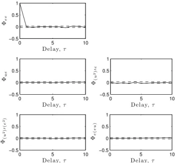
Fig. 2.Correlation tests for model validation of Eq. (2).
3 Model validation
The third stage of identifying a NARMAX model is the model validation. To do this, the identified model was sub-jected to both correlation tests (Billings and Zhu, 1989) and the model predictive performance was analyzed in both time and frequency.
3.1 Correlation validation
The correlation tests, for nonlinear systems (Billings et al., 1989), are implemented to confirm that the residuals are un-correlated with all the combinations of past values of the in-puts or the outin-puts. For a SISO NARMAX model, the model is unbiassed if the following correlations satisfy the condi-tions:
8ee(τ )=δ(τ ) ∀τ
8ue(τ )=0 ∀τ
8(u2)′e(τ )=0 ∀τ
8(u2)′(e2)(τ )=0 ∀τ
8e(eu)(τ )=0 ∀τ≥0 (3)
where 8 represents the cross-correlation between the two subscripts,τ is the delay,uis the inputC,δis the unit im-pulse function and the prime means that the mean has been removed. Figure 2 shows the results of the correlation tests.
As seen in Fig. 2, all the correlation tests are satisfied to within the confidence limits (dashed lines). Therefore the tests show that the model is unbiased.
3.2 Model predictive performance
80 85 90 95 100 105 110 115 120 125 130 −400
−300 −200 −100 0
D ay of ye ar, 2000
D
s
t
In
d
e
x
(b
la
c
k
),
O
S
A
(g
ra
y
),
(n
T
)
(a)
80 85 90 95 100 105 110 115 120 125 130
−400 −300 −200 −100 0
D ay of ye ar, 2000
D
s
t
In
d
e
x
(b
la
c
k
),
M
P
O
(g
ra
y
),
(n
T
)
(b)
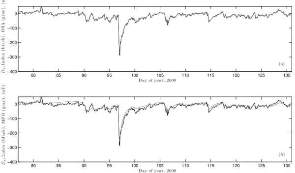
Fig. 3. (a)Measured Dst index in black and OSA Dst in grey.(b)Measured Dst index in black and MPO Dst in grey. Both for the same time period starting from 01:00 UT 17 March 2000 until 18:00 UT 9 May 2000.
model (2). The OSA uses the values of the measured Dst in-dex, in Eq. (2), to predict the next value of Dst, while the MPO uses the estimated values of Dst to predict the next value of Dst. Both the OSA and MPO are calculated from the measured values of the solar wind data. The MPO is therefore less accurate than the OSA, however, the MPO will indicate whether the model has a good long term prediction. The data employed to calculate both OSA and MPO were the uninterrupted solar wind data sections, with>1000 data points, from the start of 1998 to the end of 2008.
Figure 3 demonstrates one of the uninterrupted data sec-tions from 01:00 UT 17 March 2000 until 18:00 UT 9 May 2000. Figure 3a displays the measured Dst in black and the OSA Dst in grey. The OSA has an excellent comparability with the measured Dst, with very little difference between them. Figure 3b shows the measured Dst in black and the MPO Dst in grey. Since the MPO is calculated using the pre-vious calculations or prepre-vious predictions of Dst, rather than the measured, the MPO does not follow the measured Dst as closely as the OSA, however, it manages to follow the storms with a good agreement, forecasting the time and magnitude of the large and small storms. This indicates the model has a very good long term predictability.
Three criteria are used to analyse the the performance of the data sections. Figure 3 only displays one of the 32 un-interrupted data sections, these are not shown here due to limited space. These criteria were the normalized root mean square error (NRMSE)
ENRMSE=
v u u u u u u u u t
N X
t=1
h
y(t )− ˆy(t )2i
N X
t=1
h
(y(t )− ¯y(t ))2i
(4)
the correlation coefficient
ρyyˆ=
N X
t=1
h
(y(t )− ¯y(t ))y(t )ˆ − ¯ˆy(t )i
v u u t
N X
t=1
h
(y(t )− ¯y(t ))2i
N X
t=1
ˆ
y(t )− ¯ˆy(t )
2
(5)
and the coherency function
Cyyˆ=
Pyyˆ(f )
Pyy(f )Pyˆyˆ(f )
(6) wherey(t )is the measured andy(t )ˆ is the estimated values of the Dst at timet,N is the number of data points, the bar denotes the mean andP is the cross-spectral density of the subscripts at frequencyf.
0 0.02 0.04 0.06 0.08 0.1 0
0.2 0.4 0.6 0.8 1
Fre q ue nc y,f (hour−1)
C
o
h
e
re
n
c
y
(O
S
A
)
(a)
0 0.02 0.04 0.06 0.08 0.1
0 0.2 0.4 0.6 0.8 1
Fre q ue nc y,f (hour−1)
C
o
h
e
re
n
c
y
(M
P
O
)
(b)
Fig. 4. (a)Coherency between the measured and OSA Dst.(b) Co-herency between the measured and MPO Dst.
MPO has a lager error with higher deviation, which is ex-pected since the MPO uses the calculated Dst, rather than the measured, in Eq. (2). This indicates that the model has a good relationship with the measured Dst and that it is valid for the 11 year period.
The correlation coefficient is most often employed as an indicator of a models predictive performance and illustrates the linear dependance between the measured and estimated Dst. The mean correlation coefficient for the OSA Dst was 0.9751 with a standard deviation of 0.0114 and for the MPO Dst was 0.8403 with a standard deviation of 0.0740. The high values for the correlation coefficient and low values for the standard deviation, for both the OSA and MPO, attest that the model performs very well over the 11 year period.
Although the NRMSE and the correlation coefficient are both good indicators of a models predictive performance, they do not necessarily give a true expression of how well the model performs relevant to the objectives of this study. The objectives were to identify a model that can forecast the onset, magnitude and duration of magnetic storms. The co-herency function is able reveal the dependence between fre-quencies of the measured and estimated Dst and is therefore able to determine how well the model simulates the low fre-quencies of the magnetic storms. Since a magnetic storm can last for between 1–5 days, a large coherence at these frequen-cies would indicate that the model captures the dynamics of
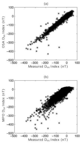
Fig. 5. (a)Measured and OSA Dst scatter plot. (b)Measured and MPO Dst scatter plot.
the storm, particularly the recovery phase. The data was di-vided into 32 bins of 1024 data point intervals, so that the coherency could be averaged over these subintervals. Fig-ure 4 displays the coherency for both the OSA (a) and the MPO (b) estimates. For the low frequencies of a magnetic storm (0.01–0.04 h−1) both the OSA and MPO have a high coherency, although the drop in coherency at higher frequen-cies, in Fig. 4b, illustrates that the model is not quite as good at forecasting the shorter storms.
depict that there are more points scattered about below the 45◦line rather than above it. This means the model tends to overestimate rather than underestimate the geomagnetic storms.
4 Discussion and conclusion
A model that forecasts the complex nonlinear dynamics of the Dst index, which employ a solar wind-magnetosphere coupling function by Boynton et al. (2011), has been iden-tified using the NARMAX OLS-ERR algorithm. The ob-jectives of this model, were to be able to forecast the time, magnitude and duration of magnetic storms accurately, i.e., predict when a storm is to occur, how strong it will be and how long it will last. Therefore the forecasting of the high frequency, small oscillation changes (e.g., between days 80 and 85 in Fig. 3) are considered unimportant in this study. Another objective for this study was to assess the ability of the coupling function by Boynton et al. (2011) as an input to model the Dst index.
A number of predictive performance criteria were used to gauge how well these objectives were achieved. The NRMSE and correlation coefficient, which are most com-monly used in the predictive performance evaluation, indi-cated a good model performance, the coherency function was high around the frequencies of 2 to 5 days, which indicated that the model is very good at picking out the storms, and the scatter plots showed that the model, although for the most part had a high correlation, tended to overestimate, rather than underestimate, the magnetic storms. The MPO scatter plateaus around zero for positive values of Dst which indi-cates that the model does not forecast the sudden commence-ments. Although unimportant to the aims of this study, the addition of more inputs could be able to identify the dynam-ics of the sudden commencements.
When comparing the results of this study to other studies that model the Dst Index, the obtained model (2) is found to be very good. The model by Boaghe et al. (2001) yielded a correlation coefficient of 0.9895 for the OSA and had a max-imum coherency of about 0.85 for the MPO. The model (2) had a marginally higher maximum coherency of about 0.9 for the MPO compared to Boaghe et al. (2001). The corre-lation coefficient for the Boaghe et al. (2001) model is high, however, the data set used for this correlation was the mea-sured Dst on which the model was trained and is only a 1000 point (hour) interval. The model (2) had an average OSA correlation coefficient of 0.9751 for 32 data sets consisting of over 76 thousand points (hours) and therefore these two OSA values cannot be compared. However, a fairer compar-ison will be to analyse the model performance for the data section shown in Fig. 3, on which the model was not trained. This gives an OSA correlation coefficient of 0.9899 which is higher than that of the model by Boaghe et al. (2001). The model by Zhu et al. (2006) was again only analysed on one
data section of 1000 data points and returned the very good results of a NRMSE of 0.4194 for the MPO and 0.1755 for the OSA. The average results from the 32 data sets for the NRMSE for the model (2) are not as good, however, the NRMSE for the data section shown in Fig. 3 returns better results than Zhu et al. (2006), a NRMSE of 0.3375 for the MPO and 0.1420 for the OSA. The Temerin and Li (2006) model has an excellent MPO correlation coefficient of 0.956. However, the model is trained on the entire 8 year period which this correlation is made. The correlation of the model Dst and the measured Dst using data on which the model was not trained, would give a more accurate indication of the model performance. This is because even a bad model can have a good fit with the data that it was trained on.
In conclusion, the coupling function by Boynton et al. (2011) performs very well at modelling the Dst index on its own and although model (2) proves more than adequate against other Dst models, there is still room for improvement. The current model only enlists one input, while the model by Temerin and Li (2006) implements many more, such as IMF and pressure terms. Therefore in the future it would be bene-ficial to employ a MISO NARMAX algorithm using the cur-rent coupling function along with more inputs such as IMF and pressure terms.
Acknowledgement. The authors would like to acknowledge the fi-nancial support from EPSRC, STFC and ERC.
Guest Editor M. Gedalin thanks two anonymous referees for their help in evaluating this paper.
References
Balikhin, M. A., Boynton, R. J., Billings, S. A., Gedalin, M., Ganushkina, N., Coca, D., and Wei, H.: Data based quest for so-lar wind-magnetosphere coupling function, Geophys. Res. Lett., 37, L24107, doi:10.1029/2010GL045733, 2010.
Billings, S. A. and Zhu, Q. M.: Nonlinear model validation using correlation tests, Int. Control J., 62, 749–766, 1989.
Billings, S., Korenberg, M., and Chen, S.: Identification of non-linear output affine systems using an orthogonal least-squares al-gorithm., Int. J. Systems Sci., 19, 1559–1568, 1988.
Billings, S., Chen, S., and Korenberg, M.: Identification of MIMO non-linear systems using a forward-regression orthogonal esti-mator, Int. J. Control, 49(6), 2157–2189, 1989.
Boaghe, O. M., Balikhin, M. A., Billings, S. A., and Alleyne, H.: Identification of nonlinear processes in the magnetospheric dy-namics and forecasting of Dst index, J. Geophys. Res., 106(A12), 30047–30066, 2001.
Boynton, R. J., Balikhin, M. A., Billings, S. A., Wei, H. L., and Ganushkina, N.: Using the NARMAX OLS-ERR algorithm to obtain the most influential coupling functions that affect the evo-lution of the magnetosphere, J. Geophys. Res., 116, A05218, doi:10.1029/2010JA015505, 2011.
Chapman, S. and Ferraro, V. C. A.: A New Theory Of Magnetic Storms, Part 1, The Initial Phase, Terr. Magn, Atmos. Electr., 36, 171–186, 1931.
Dungey, J. W.: Interplanetary Magnetic Field and Auroral Zones, Phys. Rev. Lett., 6, 47, 1961.
Hernandez, J. V., Tajima, T., and Horton, W.: Neural net forecasting for geomagnetic activity, Geophys. Res. Lett., 20, 2707–2710, doi:10.1029/93GL02848, 1993.
Kan, J. R. and Lee, L. C.: Energy coupling function and solar wind-magnetosphere dynamo, Geophys. Res. Lett., 6, 577–580, 1979. Klimas, A. J., Vassiliadis, D., Baker, D. N., and Roberts, D. A.: The organized nonlinear dynamics of the magnetosphere, J. Geophys. Res., 101(A6), 13089–13113, 1996.
Leontaritis, I. J. and Billings, S. A.: Input-Output Parametric Mod-els for Non-Linear Systems Part I: Deterministic Non-Linear Systems., Int. J. Control, 41(2), 303–328, 1985a.
Leontaritis, I. J. and Billings, S. A.: Input-Output Parametric Mod-els for Non-Linear Systems Part II: Stochastic nonlinear systems, Int. J. Control, 41(2), 329–344, 1985b.
Perreault, W. K. and Akasofu, S.-I.: A Study Of Geomagnetic Storms, Geophys. J. R. Astrom. Soc., 54, 547–573, 1978.
Price, C. P. and Prichard, D.: The nonlinear response of the mag-netosphere: 30 October 1978, Geophys. Res. Lett., 20, 771–774, doi:10.1029/93GL00844, 1993.
Prichard, D. and Price, C. P.: Spurious dimension estimates from time series of geomagnetic indices, Geophys. Res. Lett., 19, 1623–1626, doi:10.1029/92GL00630, 1992.
Sharma, A. S.: Assessing the magnetospheres nonlinear behavior – Its dimension is low, its predicability, Rev. Geophys., 33, 645– 650, 1995.
Sharma, A. S., Vassiliadis, D., and Papadopoulos, K.: Reconstruc-tion of low-dimensional magnetospheric dynamics by singular spectrum analysis, Geophys. Res. Lett., 20, 335–338, 1993. Temerin, M. and Li, X.: Dst model for 1995–2002, J. Geophys.
Res., 111, A04221, doi:10.1029/2005JA011257, 2006.
Valdivia, J. A., Sharma, A. S., and Papadopoulos, K.: Prediction of magnetic storms by nonlinear models, Geophys. Res. Lett., 23, 2899–2902, doi:10.1029/96GL02828, 1996.
Zhu, D., Billings, S. A., Balikhin, M., Wing, S., and Coca, D.: Data derived continuous time model for the Dst dynamics, Geophys. Res. Lett., 33, L04101, doi:10.1029/2005GL025022, 2006. Zhu, D., Billings, S. A., Balikhin, M. A., Wing, S., and Alleyne,