Março de 2016
João Miguel Matos Nunes
Licenciado em Ciências da Engenharia CivilAdaptive Tuned Mass Damper (ATMD)
based in shape-memory alloy
(SMA) elements.
Dissertação para obtenção do Grau de Mestre em Engenharia Civil - Perfil de Estruturas
Orientador: Professor Doutor Filipe Amarante dos Santos Professor Auxiliar, FCT/UNL
Júri:
Presidente: Prof. Doutora Zuzana Dimitrovová Arguente: Prof. Doutor Corneliu Cismasiu
“Copyright” João Miguel Matos Nunes, FCT/UNL e UNL
To my grandfather, Prof. Rogério Sanches de Matos
Acknowledgments
The present dissertation arises, not only from extensive hours of study, hard work and dedica-tion, but also as the result of a long academic journey, that would not have been accomplished without the support and assistance from many people who have either helped me or encour-aged me.
I would like to express my deepest and heartfelt recognition to my adviser, Professor Filipe Amarante dos Santos for the support, knowledge transmission and availability demonstrated throughout the development of this thesis.
I would like to thank Engineer Mirko Maraldi and Professor Luisa Molari, not only for their academic support, but also for the availability and quality care provided during my abroad study experience in Italy.
I would also like to thank Mr. Alberto Cambalacho for the assistance in the preparation of the supports used in the experimental campaign.
I leave words of appreciation to my colleagues, Inês de Carvalho, Pedro Castanho, Bruno Alcobia, Daniel Ferreira, Filipe Loureiro and André Taveira, with whom I had the pleasure of working with and share true friendship moments along the way.
I am also indebted to my comrades André Martins, Nuno Cabral, André Jorge, Diogo Canelas, Pedro Palma, Rafael Silva, Tiago Gonçalves, André Palminha, Tomás Campos and all those omitted by mistake or forgetfulness, for their support and contribute to my growth as an engineer and mainly as human being.
A special thanks to Mafalda Aquino for the unconditional support in the good and bad times, throughout my entire academic career.
Finally, I must express my gratitude towards my dear mother Teresa Matos, my father Carlos Coito, my sister Joana Nunes and the rest of my family for their love, unfailing support and inspiration.
I hope this thesis may be an encouragement for the younger members of my family (Fran-cisco and Mariana), and for all the people who read or work with it.
Abstract
The unique features of shape memory alloys (SMA) gives them an unmatched ability to be implemented in several fields of engineering. Considering their phase shift capacity, when thermoelectrically driven, SMAs assume an elastic modulus variation predicated upon two key parameters - stress and temperature.
Based on the above statement, the present dissertation aims to develop a new vibration control system, which makes use of SMAs in order to extend and improve its operational domain.
Initially, an experimental campaign is developed in order to design a mapping of the elastic modulus of a FLEXINOLR SMA sample.This mapping seeks to explore and an optimize the inclusion of shape memory alloys in vibration control systems.
In a second step, two types of ATMDs (Suppressor and TMD) are mathematically studied in order to comprise the insertion of a SMA element in the control system.
Considering the main purpose of this thesis, a particular case study structure was chosen to carry out the implementation of the new vibration control system. The selected structure consists in a footbridge built over an important highway located in the Lisbon city center, Portugal. At this stage, both the design of the SMA element and the subsequent operational limits are presented.
Afterwards, a numerical model computed in MATLAB (The Mathworks, 2014) is devel-oped to simulate the behavior of a two degrees of freedom (TDOF) system. This one provides the system’s behavior (structure + ATMD) towards a predefined harmonic request, evaluating the effects of the implementation of the new vibration control system.
Using the above mentioned numerical model, an influence analysis of both control systems was carried out. Several comparisons between the variants of each ATMD (Suppressor and TMD) where drawn, showing the positive and negative aspects of their action. In the end, a single numerical model, with the ability to excite the structure, read its behavior, identify the vibration frequencies and properly tune the control system in real time, performed a complete structural analysis.
Finally, a concluding chapter is presented, where the obtained results are discussed. This chapter also mentions the main future development prospects, that may be considered in studies conducted by other researchers.
Dissertation produced in LATEX software.
Keywords:
Resumo
As características únicas das ligas com memória de forma (LMF) conferem-lhes uma aptidão inigualável para serem implementadas em diversos ramos da engenharia. Tendo em conta a sua capacidade de alteração de fase, quando termoelectricamente accionadas, as LMF assumem uma variação do módulo de elasticidade dependente de dois parâmetros principais - tensão e temperatura.
Posto isto, a presente dissertação tem como principal objectivo o desenvolvimento de um novo sistema de controlo de vibrações, que recorre à utilização de LMFs com o intuito de alargar o domínio do seu funcionamento.
Inicialmente apresenta-se um programa experimental que contribui para a concretização de um dos sub-objectivos desta tese, isto na medida da realização de um mapeamento do módulo de elasticidade em função da temperatura de uma liga de FLEXINOL R. Este mapeamento visa uma tentativa de explorar e optimizar o comportamento das LMF.
Numa segunda fase, dois tipos de ATMDs (Supressor e TMD) são matematicamente es-tudados por forma a considerar a hipótese da inserção de um elemento constituído por LMF. Tendo em conta o objectivo principal desta dissertação, recorreu-se a um caso de estudo para realizar a implementação do sistema de controlo de vibrações. Este consiste na análise de uma ponte pedonal construída sobre um importante eixo de ligação rodoviária no centro da cidade de Lisboa, Portugal. Nesta fase, é também apresentado um dimensionamento do elemento de LMF, bem como os limites operacionais associados á sua utilização.
Seguidamente é desenvolvido um modelo numérico em MATLAB (The Mathworks, 2014) que considera a modelação de um sistema de dois graus de liberdade. Este é desenvolvido por forma a obter o comportamento do sistema (estrutura + ATMD) face a uma solicitação harmónica pré-definida, avaliando assim os efeitos da implementação do novo tipo de sistema de controlo de vibrações.
Recorrendo ao modelo numérico desenvolvido, é realizada uma análise da influência que ambos os sistemas de controlo têm no comportamento estrutural. Uma série de comparações são realizadas entre as variantes de cada ATMD, evidenciando os aspectos positivos e negativos associados. É também apresentada uma análise estrutural feita com um modelo numérico completo, com a capacidade de excitar a estrutura, ler o seu comportamento, identificar as frequências de vibração e sintonizar correctamente o sistema de controlo em tempo real.
Para finalizar, é apresentado um capítulo conclusivo, onde os resultados obtidos nesta dissertação são comentados. Neste capítulo são também referidas as principais perspectivas de desenvolvimento futuro, que podem ser consideradas em estudos realizados por outros investigadores.
Dissertação produzida em LATEX software.
Palavras chave:
Contents
Contents xi
List of Figures xv
List of Tables xix
List of Abbreviations, Acronyms and Symbols xxi
1 Introduction 1
1.1 Problem Description . . . 1
1.2 Objectives and Scope . . . 2
1.3 Dissertation Outline . . . 3
2 Shape Memory Alloys 5 2.1 Introduction to Shape Memory Alloys (SMA) . . . 5
2.2 General aspects of Shape Memory alloys . . . 6
2.2.1 Operating principles of SMAs . . . 6
2.2.2 Superelasticity . . . 7
2.2.3 Shape Memory effect . . . 7
2.3 Shape Memory Alloys in Civil Engineering . . . 9
2.4 Constitutive Models for Shape-Memory Alloys . . . 9
2.4.1 Introduction . . . 9
2.4.2 Kinetic law . . . 10
2.4.3 Mechanical law . . . 11
2.4.3.1 Voight scheme . . . 11
2.4.3.2 Reuss scheme . . . 12
2.4.4 Constitutive Model Summary . . . 12
3 Mapping of the SMAs Modulus of Elasticity 13 3.1 Introduction . . . 13
3.3 Experimental mapping - Young modulus of the SMA wire . . . 14
3.3.1 Experimental Device . . . 14
3.3.2 Experimental Method . . . 17
3.3.3 Results . . . 19
3.4 Numerical approach - Young modulus of the SMA wire . . . 22
3.4.1 Kinetic law . . . 22
3.4.2 Mechanical law . . . 26
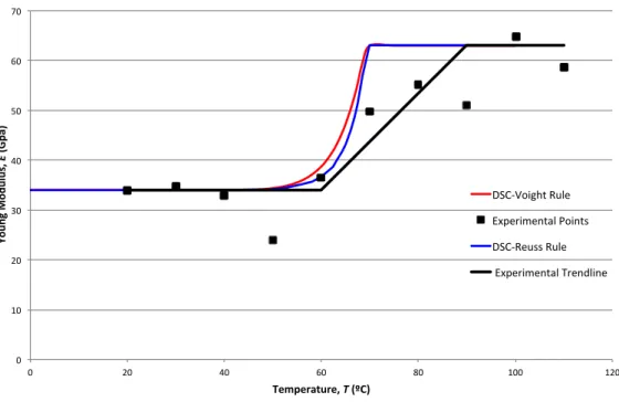
3.5 Experimental approach Vs. Numerical approach - Young modulus of the SMA wire . . . 27
4 Vibration Control Systems - Adaptive Tuned Mass Damper 29 4.1 Introduction . . . 29
4.2 The Undamped Dynamic Vibration Absorber - Vibration Suppressor . . . 30
4.3 The Damped Vibration Absorber - Tuned Mass Damper (TMD) . . . 33
4.4 Suppressor Vs. TMD . . . 35
5 Implementation of an Adaptive Tuned Mass Damper in a Footbridge 37 5.1 Introduction . . . 37
5.2 Case Study - Footbridge . . . 38
5.2.1 Footbridge Geometry . . . 38
5.2.2 Dynamic behavior . . . 39
5.2.3 Dynamic Actions and Structural Response . . . 39
5.3 Implementation of the Vibration Control System to the Case Study . . . 41
5.3.1 Design of a TMD with constant stiffness - Case Study . . . 41
5.3.2 Design of a Vibration Suppressor with constant stiffness - Case Study 42 5.4 Design of SMA Wires - Control System "spring" . . . 43
5.5 SMA Wire Operating Limits - Control systems with variable stiffness . . . 46
5.5.1 Suppressor with Variable Stiffness . . . 46
5.5.2 TMD with Variable Stiffness . . . 48
6 Numerical Analysis of a Simplified Two Degree of Freedom Dynamic System 51 6.1 Introduction . . . 51
6.2 Simplified Two Degree of Freedom Dynamic System . . . 51
6.3 Short-time Fourier transforms . . . 52
6.3.1 Short-time Fourier transforms - Description . . . 52
6.3.2 Short-time Fourier transforms - Implementation . . . 53
6.3.2.1 STFT in the Two Degree of Freedom Dynamic System . . . . 54
6.4 Two Degree of Freedom Dynamic System - MATLAB Implementation . . . . 56
6.4.1 Dynamic Analysis Model - MATLAB . . . 56
7 Results of the Numerical Analysis 61 7.1 Introduction . . . 61
7.2 Initial Case . . . 61
7.3 Suppressor . . . 62
7.3.1 Suppressor with Constant Stiffness (SCS) Vs. Suppressor with Variable Stiffness (SVS) . . . 62
Contents
7.4 Tunned Mass Damper (TMD) . . . 67 7.4.1 TMD with Constant Stiffness (TMDCS) Vs. TMD with Variable
Stiff-ness (TMDVS) . . . 67 7.5 TMD Vs. Suppressor . . . 69 7.5.1 Tuned Mass Damper (TMDVS) Vs. Suppressor (SVST) . . . 69 7.6 TMD and Suppressor - STFT algorithm in the Output response signal . . . . 70 7.6.1 Suppressor (SVST) . . . 71 7.6.2 Tuned Mass Damper (TMDVS) . . . 72
8 Summary, Conclusions and Future Work 75
8.1 Summary and Conclusions . . . 75 8.2 Future Works . . . 78
Bibliography 79
Appendix 83
A Experimental approach - SMA wire Young Modulus Mapping A1
B Proportional-Integral-Derivative (PID) Control Algorithm B1
C Numerical approach - SMA wire Young Modulus Mapping C1
D Design of SMA Wires Under Constant Force D1
E Short-time Fourier transforms - MATLAB implementation E1
List of Figures
2.1 Phase alternation with respect to temperature. [38] . . . 6
2.2 Superelasticity effect. Residual strain: u0 = 0 ; Temperature variation: ∆T ≈0. (Adapted from [33]). . . 7
2.3 Shape Memory effect. Residual strain: u0 >0; Temperature variation: ∆T >0. (Adapted from [33]). . . 8
2.4 Properties of Shape-memory-alloys. Relations between Stress, Strain and Temper-ature. [34] . . . 8
2.5 Mechanical models for SMAs, [6] . . . 11
3.1 FLEXINOLR actuator wire. . . . 14
3.2 Experimental Device. . . 15
3.3 National Instruments NI PXI-1052 controller and kaise DC power supply hy3005d. 16 3.4 Baumer Photoelectric sensor CH-8501 Class 2 laser, Target and Leveler device. . 16
3.5 Stress - Strain curve for a 20oC temperature . . . . 18
3.6 Stress-Strain curves obtained for the considered temperature range. . . 20
3.7 Modulus of elasticity as function of temperature. . . 21
3.8 DSC analysis (from [32]) . . . 22
3.9 Extraction of the Heat Flux values from the DSC curve. . . 23
3.10 Unsmeared Heat Flux of the M →A transformation. . . 23
3.11 Austenite phase fraction evolution during the M →A transformation. . . 24
3.12 Austenite phase fraction - Equation (2.3), f(T, g, ν, Tm). . . 24
3.13 Suitability of equation (2.3) to the graphical data of Figure 3.11. . . 25
3.14 Voight scheme - Modulus of elasticity as function of temperature. . . 26
3.15 Reuss scheme - Modulus of elasticity as function of temperature. . . 26
3.16 Experimental approach Vs. Numerical approach - Young modulus of the SMA wire. 27 4.1 Main System and the Undamped Dynamic Vibration Absorber. . . 30
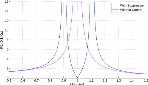
4.2 Amplitude of the main system motion with and without Suppressor. . . 32
4.3 Main System and the Damped Vibration Absorber. . . 33
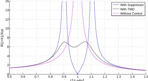
4.5 Amplitude of the main system motion with Suppressor, with TMD and without
control system. . . 35
5.1 Footbridge over the Avenida Marechal Gomes da Costa, T. Krus, [15]. . . 38
5.2 Three dimensional view of the footbridge model, T. Krus, [15]. . . 38
5.3 Configuration of the 2nd vibration mode of the structure - 1st vertical vibration mode: f=3,46 Hz - T. Krus, [15]. . . 39
5.4 Suppressor Operating Limits. . . 47
5.5 TMD Operating Limits. . . 50
6.1 Vibration Suppressor - Two Degree of Freedom Dynamic System. . . 52
6.2 TMD - Two Degree of Freedom Dynamic System. . . 52
6.3 Implementation of the STFT in the control algorithm. . . 53
6.4 Sinusoidal force where the frequency changes from 5 Hz to 3,03 Hz - Input force signal. . . 54
6.5 Resonance situation triggered in the structure of the case study - Output response signal. . . 54
6.6 Short-time Fourier transform spectrum - Input force signal. . . 55
6.7 Frequency tracking - Input force signal. . . 55
6.8 Short-time Fourier transform spectrum - Output response signal. . . 55
6.9 Frequency tracking - Output response signal. . . 55
7.1 Acceleration-time graphic for the case study structure. . . 61
7.2 Amplitude of the main system motion with Suppressor (SCS) designed for a 3,03 Hz natural frequency. . . 63
7.3 Sinusoidal force where the frequency changes from 3,03 Hz to 3,36 Hz. (0 <Time<30 seconds →f = 3,03 Hz) ; (30<Time <60 seconds→f = 3,36 Hz). 63 7.4 Acceleration-time graphic for the Suppressor with Constant Stiffness (SCS). k2 = 159,477 kN/m is maintained during the two phases. . . 64
7.5 Acceleration-time graphic for the Suppressor with Variable Stiffness (SVS). In the 1st phasek 2 = 159,477 kN/m and in the 2nd phasek2 = 196,106 kN/m . . . 64
7.6 Amplitude of the main system motion with Suppressor. Stiffness transition and Operating Limits representation. . . 65
7.7 Acceleration-time graphic for the Suppressor (SVS) Without Stiffness Transition. k2 = 241,67 kN/m is maintained during the two phases. . . 66
7.8 Acceleration-time graphic for the Suppressor (SVS) With Stiffness Transition. In the1st phasek 2 = 241,67 kN/m and in the 2nd phase k2 = 112,07 kN/m. . . 66
7.9 Amplitude of the main system motion with the TMD (TMDCS) designed for a 3,03 Hz natural frequency. Operating limits displayed (vertical lines). . . 67
7.10 Acceleration-time graphic for the TMD with Constant Stiffness (TMDCS). k2 = 147,1 kN/m is maintained during the two phases. . . 68
7.11 Acceleration-time graphic for the TMD with Variable Stiffness (TMDVS). In the 1st phasek2 = 147,1 kN/m and in the 2nd phasek2 = 163,1 kN/m. . . 68
7.12 Acceleration-time graphic for the TMDVS action. . . 69
7.13 Acceleration-time graphic for the SVST action. . . 69
7.14 Sinusoidal force where the frequency changes from 5 Hz to 3 Hz. . . 70
List of Figures
7.16 Acceleration-time graphic for the SVST action - STFT in the Output response signal. . . 71 7.17 Short-time Fourier transform spectrum - Output response signal of the structure
with TMDVS. . . 72 7.18 Frequency tracking - Output response signal of the structure with TMDVS. . . . 72 7.19 Acceleration-time graphic for the TMDVS action - STFT in the Output response
signal. . . 73
A.1 Stress-Strain curve for 20oC . . . . A2
A.2 Stress-Strain curve for 30oC . . . . A2
A.3 Stress-Strain curve for 40oC . . . . A3
A.4 Stress-Strain curve for 50oC . . . . A3
A.5 Stress-Strain curve for 60oC . . . . A4
A.6 Stress-Strain curve for 70oC . . . . A4
A.7 Stress-Strain curve for 80oC . . . . A5
A.8 Stress-Strain curve for 90oC . . . . A5
A.9 Stress-Strain curve for 100oC . . . . A6
A.10 Stress-Strain curve for 110oC . . . . A6
B.1 Proportional-Integral-Derivative (PID) Controller layout. . . B2
C.1 Heat Flux - PlotDigitizer analisys. . . C2 C.2 Heat Flux [mW/mg]. . . C2 C.3 Unsmeared Heat Flux of the M →A transformation. . . C2 C.4 Transformation rate. . . C3 C.5 Austenite phase fraction evolution (DSC analysis). . . C3 C.6 Austenite phase fraction (Equation (2.3)). . . C3 C.7 Suitability of equation (2.3) to the graphical data of Figure 3.11. Figures C.5
and C.6 overlay. . . C4 C.8 Voight scheme - Modulus of elasticity as function of temperature. . . C5 C.9 Reuss scheme - Modulus of elasticity as function of temperature. . . C5 C.10 Experimental approach Vs. Numerical approach - Young modulus of the SMA wire. C6
D.1 Reuss scheme - Modulus of elasticity as function of temperature. . . D3 D.2 Stiffness mapping as function of temperature. . . D3
List of Tables
2.1 Austenite and Martensite phases. . . 6
2.2 Constitutive Model for SMAs - Summary . . . 12
3.1 Wire length with no loading. . . 20
3.2 SMA wire Test Results . . . 21
3.3 Equation (2.3) fitting parameters. . . 24
5.1 Common values of damping ratio ζ for footbridges, [20]. . . 39
5.2 Distributed loads regarding the pedestrians mass, [15] . . . 40
5.3 Natural frequency of the structure. . . 40
5.4 Time-history force function for the 1st Vertical mode of a Class I footbridge, con-sidering the Sétra Model [35]. . . 40
5.5 Optimal parameters of the vertical TMD. . . 42
5.6 Optimal parameters of the vertical suppressor. . . 43
5.7 Stress influence in the wire’s strain/stiffness . . . 45
5.8 Temperature influence in the wire’s strain/stiffness . . . 45
5.9 Suppressor’s operating limits . . . 48
5.10 TMD’s operating limits . . . 50
A.1 Test Temperature: 20oC - experimental results . . . . A2
A.2 Test Temperature: 30oC - experimental results . . . . A2
A.3 Test Temperature: 40oC - experimental results . . . . A3
A.4 Test Temperature: 50oC - experimental results . . . . A3
A.5 Test Temperature: 60oC - experimental results . . . . A4
A.6 Test Temperature: 70oC - experimental results . . . . A4
A.7 Test Temperature: 80oC - experimental results . . . . A5
A.8 Test Temperature: 90oC - experimental results . . . . A5
A.9 Test Temperature: 100oC - experimental results . . . . A6
A.10 Test Temperature: 110oC - experimental results . . . . A6
C.2 Baseline-corrected-unsmeared Heat Flux values. . . C2 C.3 Austenite phase fraction (DSC analysis). . . C3 C.4 Fit parameters. . . C3 C.5 Austenite phase fraction (Equation (2.3)). . . C3 C.6 Voight scheme (E vs. T). . . C5 C.7 Young Modulus in Martensite/Austenite phase. . . C5 C.8 Reuss scheme (E vs. T). . . C5 C.9 Young Modulus in Martensite/Austenite phase. . . C5
List of Abbreviations, Acronyms and
Symbols
Abbreviations and Acronyms ATMD Adaptive Tuned Mass Damper
DFT Discrete Fourier Transform
DOF Degree of Freedom
DSC Differential Scanning Calorimetry
FCT Faculdade de Ciências e Tecnologias
LMF Liga com Memória de Forma
MDOF Multi Degree of Freedom
NiTi Nickel-Titanium alloy
PID Proportional?Integral?Derivative controller
PSD Power Spectral Density
SCS Suppressor with Constant Stiffness
SDOF Single Degree of Freedom
SMA Shape Memory Alloy
STFT Short Time Fourier Transform
SVS Suppressor with Variable Stiffness
SVST Suppressor with Variable Stiffness and stiffness Transition
TMD Tuned Mass Damper
TMDCS Tuned Mass Damper with Constant Stiffness
TMDVS Tuned Mass Damper with Variable Stiffness
Symbols
ξ Martensite phase fraction
ζ Damping ratio
u Displacement vector
A Austenite
M Martensite
Ms Martensitic phase Start
Mf Martensitic phase Finish
As Austenitic phase Start
Af Austenitic phase Finish
σ Stress
σM Martensitic Stress
σA Austenitic Stress
E Modulus of Elasticity (Young)
Ew Modulus of Elasticity of the wire
EM Modulus of Elasticity in Martensitic phase
EA Modulus of Elasticity in Austenitic phase
ε Strain
εM Strain in Martensitic phase
εA Strain in Austenitic phase
εL Maximum residual Strain
Kp Proportional gain
Ki Integral gain
Kd Derivative gain
e Error
t Instantaneous time
τ Variable of integration
g Fit parameter
List of Abbreviations, Acronyms and Symbols
Tm Fit parameter
T Temperature
Tw Wire temperature
L Length
∆L Length variation
f(T) Austenite phase fraction
m Mass
c Damping
k Stiffness
m1 Mass of the primary system (structure)
m2 Mass of the secondary system (ATMD)
c1 Damping coefficient of the primary system (structure)
c2 Damping coefficient of the secondary system (ATMD)
k1 Stiffness of the primary system (structure)
k2 Stiffness of the secondary system (ATMD)
P0 Amplitude of the force function
f Vibration Frequency [Hz]
ω Angular frequency [rad/s]
ω1 Angular frequency of the primary system (structure)
ω2 Angular frequency of the secondary system (ATMD)
x Displacement
˙
x Velocity
¨
x Acceleration
X1 Amplitude of the displacement of the primary system (structure)
X2 Amplitude of the displacement of the secondary system (ATMD)
Xst Static deflection of the primary system (structure)
r1 Ratio between the excitation frequency and the frequency of the primary system
r2 Ratio between the excitation frequency and the frequency of the secondary system
µ Mass ratio between the primary and secondary system masses
ζ2 Damping ratio of the TMD
ζ2,opt Optimum Damping ratio of the TMD
ω2,opt Optimal frequency of the TMD
amax Maximum acceleration
A Area (cross section)
d Diameter
KM Stiffness in Martensitic phase
KA Stiffness in Austenitic phase
S Stroke
M Mass Matrix
K Stiffness Matrix
C Damping Matrix
u0(t) Initial displacement vector
˙
u0(t) Initial velocity vector
P(t) Excitation force vector
γ Newmark’s method stability coefficient
Chapter 1
Introduction
"We shape our buildings, thereafter they shape us." - Winston Churchill
1.1
Problem Description
In the past few years, footbridges have evolved to overcome larger spans and achieve greater lightness to perfectly suit in the surrounding environments. Footbridges are usually steel structures, with great flexibility and low damping ratios, directly influencing their dynamic behavior. The decrease in the stiffness, often leads to structures with lower natural frequencies and with an increased risk of resonance.
With the purpose of mitigating this negative impact on structures, different approaches have been studied over the past few years. A well known vibration control approach is based in the use of Tuned Mass Dampers (TMD). A TMD reduces the vibration of a system with a comparatively lightweight component, stabilizing it against violent motions caused by harmonic vibrations. Roughly speaking, TMDs are currently tuned to either move the main mode away from a troubling excitation frequency, or to add damping excluding the possibility of resonance.
The main problem regarding TMDs usage is related to the fact that they are designed only to be tuned to the structure’s natural frequency, which introduces the resonance effect. Therefore, their effect won’t become so sharp when the harmonic action comprises other range of frequencies.
In order to overcome the above mentioned weakness, several control systems have been studied. Among the ones reported in the literature, one highlights a device studied by N. Varadarajan and S. Nagarajaiah [42] and S. Nagarajaiah and E. Sonmez [25], where a vibration control system with a property of "variable stiffness" was developed. This "variable stiffness" property allows a correct tuning of the device for a wider range of frequencies.
1.2
Objectives and Scope
Regarding the previously exposed problematic, the present dissertation aims to develop a new approach on a vibration control system, which increases the performance towards a wider range of vibration exposure. In order to achieve the above mentioned primary objective, different work stages with secondary objectives were considered.
• The first task will address the temperature/stress mapping of a SMA element with respect to its elastic modulus. For this, both an experimental and a numerical approach will be developed.
• In a second stage of the work, two ATMD vibration control systems will be studied considering the hypothesis of the inclusion of a SMA element in the system.
• The third stage regards the full definition of a numerical model based on a simplified two degree of freedom dynamic system implemented in MATLAB (The Mathworks, 2014), to simulate the behavior of the composed structural system (footbridge + ATMD), associated with a dynamic loading.
1.3. Dissertation Outline
1.3
Dissertation Outline
The content of the dissertation is organized into the following chapters:
Chapter 1 - General approach to the subject of the present dissertation.
Chapter 2 - General introduction to SMAs, including a description of the supere-lasticity and shape-memory effects, triggered by martensitic transformations. SMAs applications in Civil Engineering. Constitutive models for SMAs and definition of the Mechanical and kinetic governing laws considered in this document.
Chapter 3- Detailed description of the Experimental and Numerical approaches on the definition of the Young Modulus Mapping of FLEXINOLR actuator wires. Reference to the proportional-integral-derivative (PID) algorithm used in the experimental tests. Review and application of the defined constitutive model. Comparisons between the different approaches and results.
Chapter 4- Introduction to the vibration control systems (Suppressor and TMD) stud-ied in this document. Mathematical definition of those two vibration control systems, according to the studies reported by Den Hartog [12].
Chapter 5 - Simplified overview of this document case study. Review of the studies reported by T. Krus [15]. Geometry, structural aspects and analysis of the case study footbridge. Implementation of a vibration control system in the Footbridge. Inclusion of the "variable stiffness" property in the considered vibration control systems, using SMAs, in order to increase their performance. Definition of the operating limits of both ATMDs.
Chapter 6 - Numerical implementation of the active control strategy, based on a Splified Two Degree of Freedom Dynamic System. MATLAB (The Mathworks, 2014) im-plementation of the two Vibration Control Systems (Suppressor and TMD) previously studied. Definition and numerical implementation of a frequency tracking algorithm based on short-time Fourier transforms (STFT), to determine the real-time frequency of a sinusoidal signal as it changes over time.
Chapter 7- Analysis of the results yielded by the numerical tests performed. Definition of the initial vibration problems of this case study footbridge, considering the developed numerical model. Single Numerical Model with the STFT frequency tracking algorithm in the Output response signal of the structure.
Chapter 2
Shape Memory Alloys
2.1
Introduction to Shape Memory Alloys (SMA)
In the present chapter, the main concepts underlying the definition of Shape Memory Alloys and their applications in Civil Engineering, are introduced. In the small group of smart materials, Shape Memory Alloys (SMAs) belong to a class that gives them the capacity to memorize their previous characteristics when subjected to certain kinds of stimulus such as thermomechanical variations. Taking advantage of their unique features and considering the research being developed, SMAs have drawn significant attention in a wide range of commercial applications, in the latest years.
SMAs are characterized by two main thermo-mechanical properties, the Shape Memory Effect and Superelasticity. The application of both properties, as well as the functioning of the material itself, is highly related with a diffusionless phase transformation, characteristic of SMAs, called martensitic transformation. Due to this transformation, the material atoms rearrange themselves differently according to external factors like Temperature or Stress vari-ations. The two main types of atom rearrangements, yield to two different phases, Martensitic and Austenitic phase.
2.2
General aspects of Shape Memory alloys
Although SMAs can be composed by different chemical elements, this document only considers the ones composed by Nickel and Titanium alloys (NiTi SMAs), mostly known as Nitinol wires. As mentioned in this chapter’s introduction, SMAs are characterized by two important thermo-mechanical properties:
• Superelasticity;
• Shape-Memory effect.
Both mentioned thermo-mechanical properties are based upon martensitic transforma-tions. Those properties and transformations are described in detail in the following sectransforma-tions.
2.2.1 Operating principles of SMAs
SMAs are characterized by comprising two main phases, where the internal organization of the crystals changes according to Temperature/Stress variations:
• Austenitic Phase;
• Martensitic Phase.
Both phases are further described in Table 2.1.
Table 2.1: Austenite and Martensite phases.
Austenite Martensite
"Elastic behavior" phase "Plastic behavior" phase "Stronger" phase "Weaker" phase Stable at high temperatures Stable at low temperatures
Cubic crystal structure Monoclinic crystal structure
In order to clarify the operation of SMAs, the Figure 2.1 diagram is presented, illustrating the transition between the two mentioned crystallographic phases as function of temperature.
2.2. General aspects of Shape Memory alloys
Figure 2.1 presents the relation between the Temperature (T) and the martensite phase fraction (ξ). The martensite phase fraction comprises values between 0 and 1, where 1 corre-sponds to the complete martensitic phase and 0 correcorre-sponds to the complete austenitic phase. With this, it is possible to observe that as the temperature increases, a phase transition from martensite to austenite occurs in the alloy. In order to define the start and finish point of each phase transition process, the following transformation temperatures are presented:
Ms - Martensitic phase Start.
Mf - Martensitic phase Finish.
As - Austenitic phase Start.
Af - Austenitic phase Finish.
2.2.2 Superelasticity
The Superelasticity thermo-mechanical property of SMAs is a result of the internal rearrange-ment of the alloy crystals which gives to the SMA a higher elastic recovery in comparison to the metals and commonly used alloys. In SMAs, Superelasticity is associated with recoverable strains up to 8% during a mechanical cycle of loading and unloading that, when compared to 0.2% of the common alloys, represents a considerable increase.
To illustrate this phenomenon, one considers the example of a single SMA column (in the austenitic phase) with a fixed support at its basis and with the other edge free (Figure 2.2).
Figure 2.2: Superelasticity effect. Residual strain: u0= 0 ; Temperature variation: ∆T ≈0.
(Adapted from [33]).
When a single load is applied at the free top edge of the column, it triggers a deformation process in that element. Due to its superelastic properties, when the load is removed, the column returns to its initial configuration, without any residual deformation.
2.2.3 Shape Memory effect
As the name implies, this property allows the alloy to recover its undeformed configuration after being subjected to a positive variation of its temperature. This positive variation of temperature must be within a range of values that allows martensitic transformations to occur. SMAs can be subjected to many shape-memory cycles without any loss of resistant stress.
Figure 2.3: Shape Memory effect. Residual strain: u0 >0 ; Temperature variation: ∆T >0.
(Adapted from [33]).
With the application of the single load, the column suffers an induced deformation process and when reaching a certain stress value, it enters into a plastic regime.
Unlike in the superelasticity phenomenon, when the load is removed, the column does not return to its original shape. This is due to the fact that the column comprised a plastic deformation and thus, a residual strain needs to be considered (the column recovers only part of the total strain to which it was subjected).
However, a positive temperature variation can be introduced into the system causing a phase transition from martensite to austenite, and then the structure will be able to completely recover its original shape. This phenomenon is called the shape memory effect.
The above represented cycle may be repeated many times without changes in the material properties.
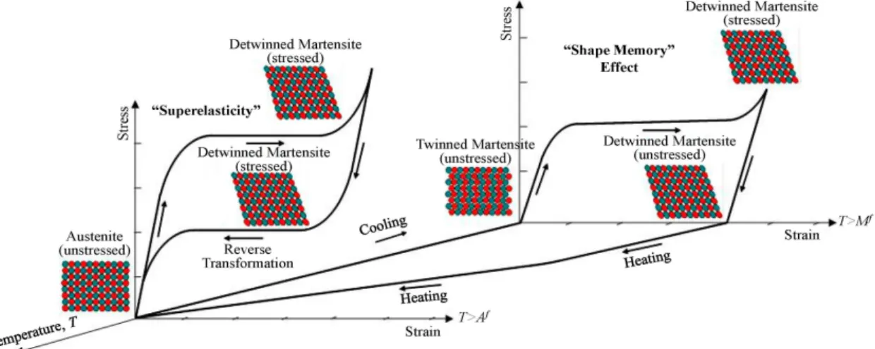
To summarize the whole operation of NiTi alloys, Figure 2.4 presents a sequence of marten-sitic transformations which demonstrate the superelastic and shape memory behavior of this type of SMA.
Figure 2.4: Properties of Shape-memory-alloys. Relations between Stress, Strain and Tem-perature. [34]
2.3. Shape Memory Alloys in Civil Engineering
phase to an austenitic one. Due to the "shape-memory effect", the alloy is now able to recover its undeformed shape. When in the austenitic phase, one applies a stress variation, the material will experience the expected deformation, but this time, upon the removal of the applied stress, it is able to completely recover the undeformed shape. This phenomenon occurs due to the "Superelasticity" property, characteristic of the austenitic phase.
2.3
Shape Memory Alloys in Civil Engineering
Nowadays, SMA’s applications in civil engineering structures are quite occasional, even though, they begin to be more frequently seen in several applications. Perhaps the most relevant one is the application of SMA’s in vibration control devices, mainly implemented in buildings and footbridges, which is the main subject of the present dissertation.
The application of these alloys is also increasing, in structural rehabilitation. The ability of this material to recover its original shape can be very useful in structural rehabilitation and also in the field of self-rehabilitation of damaged structural elements.
Most of the SMAs implementation examples in civil engineering structures, can be ob-served in Italy, with several successful cases of real applications of SMA materials. Most of these applications are related with the rehabilitation of historical structures damaged by seismic events [22] [13] [38].
Some studies, regarding the use of SMAs in vibration control systems, have also been conducted in other areas of civil engineering, such as Tensegrity structures [30]. SMAs are also often used to improve the behavior of several types of structures [1] [27], or even in specific structural elements [40].
Even though the use of SMAs may increase the structures performance, it always requires a substantial amount of material. This may be an important restraint to their implementation due to their high price, when compared with other conventional construction materials [31].
2.4
Constitutive Models for Shape-Memory Alloys
2.4.1 Introduction
In order to describe the highly complex behavior of Shape-Memory Alloys, different consti-tutive models have been developed. Each of these models takes into account the properties of SMAs that must be considered for a particular study, making the model more suitable for the study in concern.
These models are usually constituted by two main coupled laws, the Kinetic Law and the Mechanical Law. The Kinetic Law is used to describe the evolution of the phase fraction as a function of stress and temperature, governing the process of the crystallographic transfor-mation between phases, while the Mechanical Law is mainly concerned with the stress-strain behavior of the alloy itself.
2.4.2 Kinetic law
Several phenomenological kinetic equations have been proposed in the literature to describe kinetic data of different constitutive models for NiTi SMAs. These equations cover a wide range of mathematical approaches to the kinetic data, ranging from Exponential laws [39], Cosine based laws [16], Linear and Tangentially laws [14] and even Square-rooted based laws [17].
In order to mathematically describe the evolution of the degree of Martensitic transfor-mation regarding the temperature, the kinetic law presented by Nikolay Zotov, Vladimir Marzynkevitsch and Eric J. Mittemeijer [47] is adopted in this work.
This model is based on the kinetic data (for Austenite fraction) obtained by DSC (differ-ential scanning calorimetry) during the M → A transformation in order to obtain a better agreement with experimental data than the existing empirical models. Due to the fact that the transformation issues of NiTi SMAs depend on the composition and on the thermo-mechanical treatment of the alloys, in the referred article, the DSC analysis was applied to two NiTi SMAs with different compositions (nearly-equiatomic NiTi SMAs (50.1 at.% Ni) and Ni-rich NiTi SMA (50.7 at.% Ni)), but for the sake of simplicity, the present study will only focus on the nearly-equiatomic NiTi SMAs.
With the DSC test results obtained (see Figure 3.8), the degree of transformation can be determined from the enthalpy of the transformation, expressed by the area of the DSC graphic peak. According to [47], a baseline-corrected and unsmeared DSC curve, can be obtained using:
Fu(t) =Fm(t) +
τ dFm(t)
dt (2.1)
where Fm(t) ∼ d∆dtH, ∆H is the enthalpy change of the SMA specimen and τ is a time constant.
In order to preform the kinetic analysis of the austenite formation as a function of temper-ature, the data obtained from the DSC curves described above (mainly the baseline-corrected and unsmeared DSC curve given by equation (2.1)) can be used to find the austenite phase fraction applying:
f(T) =
1 ∆HA
Z T
0
Fu(y)dy (2.2)
Where∆HA is the total enthalpy change of the M → A phase transformation andFu is the unsmeared heat flux (2.1).
To obtain a more realistic description of the experimental kinetic data than the existing SMA kinetic models, Nikolay Zotov, Vladimir Marzynkevitsch and Eric J. Mittemeijer [47] proposed:
f(T) = 1
(1 + exp(−gν(T −Tm)))
1
ν (2.3)
Equation (2.3) describes the evolution of the Austenite phase fraction as function of Tem-perature, and it is ruled by three fit parameters (g, ν, Tm) that have simple physical mean-ings. Tm determines the temperature corresponding to the maximum transformation rate
(df /dT)max,g and ν determine the transformation rate(df /dT).
2.4. Constitutive Models for Shape-Memory Alloys
2.4.3 Mechanical law
In order to perform a stress-strain (σ−ε) analysis related to the temperature (T) and marten-site phase fraction (ξ) of SMAs, a mechanical law is implemented. There are three main ap-proaches that consider transformation phase fraction to be related with the elastic fraction of the response. According to [6], if the elastic fraction of the response is limited to the austenite phase, a simple serial model is obtained (see Figure 2.5a). If a parallel distribution of austenite and martensite phases is considered, a Voight scheme is obtained (see Figure 2.5b). If a peri-odical distribution of austenite and martensite phases within the material, orthogonal to the direction of the applied stress is considered, the Reuss scheme is obtained (see Figure 2.5c).
(a) Simple serial model (b) Voight scheme (c) Reuss scheme
Figure 2.5: Mechanical models for SMAs, [6]
Due to the interest of reporting the evolution of the Young Modulus regarding the tem-perature, is necessary to take into account the two main phases that occur in this material, as well as the length of variations between phases. Therefore, this document will only address the Voight and Reuss schemes which contemplate those two different crystallographic phases, austenite and martensite.
2.4.3.1 Voight scheme
Assuming that the austenitic and martensitic elastic strains are equal (εelast=εM =εA), the mechanical law governing the behavior of the material can be expressed as:
σ=ξ σM+ (1−ξ)σA (2.4)
and considering Hooke’s Law (σ=E ε), it is possible to obtain the following relationship, or "rule of mixture" [36]:
Ew =ξ EM + (1−ξ)EA (2.5)
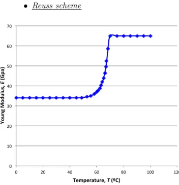
2.4.3.2 Reuss scheme
According to Reuss scheme, the prerequisite for the formulation of its mechanical law is based on the assumption that the total strain of the material depends on the percentage of phase associated with it, i.e:
ε=ξ εM + (1−ξ)εA (2.6)
Considering the total stress in each phase, the individual phase strains are given by:
εA= EσA andεM = EσM +εL. Equation (2.6) results in:
σ= EAEM
ξ EA+ (1−ξ)EM
(ε−εLξ) (2.7)
WhereεL is the maximum residual strain in the material. Considering Hooke’s Law once again, the Young Modulus relation for the Reuss scheme can be expressed as:
Ew= EAEM ξ EA+ (1−ξ)EM
(2.8)
2.4.4 Constitutive Model Summary
In order to summarize the considered constitutive model as well as its constitutive laws, Table 2.2 is presented below.
Table 2.2: Constitutive Model for SMAs - Summary
Kinetic Law
[47] f(T) = 1(1+exp(−gν(T−Tm))) 1 ν (2.3)
Mechanical Laws
Voight Ew =ξ E
M+ (1−ξ)EA (2.5)
Reuss Ew = EAEM
Chapter 3
Mapping of the SMAs Modulus of
Elasticity
3.1
Introduction
The behavior of the SMAs Young’s modulus in a thermal cycle is a very interesting issue for the study of the application of these materials. Several articles in the literature already describe this specific behavior of SMA wires [47] [36].
Hereupon, one considers the mapping of the SMAs Young Modulus as the leading objective of the present chapter.
Although each crystallographic phase has a particular value of Young’s Modulus associated with it, a non-linear and hysteretic dependence of the wire modulus Ew = Ew(T), which occurs during the phase transition interval, is considered to be the focus of the present chapter. In order to do this, two different methods were used. First, an experimental test was performed, where the modulus of elasticity of the NiTi wire was calculated based on the Hooke’s law concepts, while in the second method, the calculation of the modulus of elasticity relied upon the use of the constitutive models specified in section 2.4, that have been based on a DSC analysis performed on the same NiTi wires.
3.2
SMA wire characteristics
The SMA wires used in this work were provided by Dynalloy, Inc. These small diameter
FLEXINOL R wires are made of Nickel and Titanium and they are able to contract when electrically driven or heated. Their ability to flex/shorten is considered a characteristic of SMAs, which dynamically change their internal structure when submitted to certain temper-atures.
The modulus of elasticity of SMA wires can vary considerably with composition, elon-gation, training, and temperature. For NiTinol, in the low temperature phase (Martensite), it varies between 28-40 GPa and in the high temperature phase (Austenite), it is around 83 GPa.
According to the FLEXINOL R catalog the transformation temperature of the actuator wire is set around 60◦C and 110◦C (As = 90oC). This allows an easy heating process with
modest electrical currents applied directly through the wire, and a quick cooling process to temperatures below the transformation temperature as soon as the current is stopped.
Figure 3.1: FLEXINOL R actuator wire.
Relevant physical properties ofFLEXINOLR:
• Diameter: 0,5mm;
• Density: 6
,45g/cm
3 ;
• Specific heat: 0,2cal/g.
oC;
• Melting point: 1300◦C;
• Thermal Conductivity: 0,18W/cm
◦C;
• Thermal expansion coefficient:
– Austenitic phase: 11,0×10
−6
/◦C;
– Martensitic phase: 6,6×10
−6
/◦C;
• Approximate electrical resistance:
– Austenitic phase: 100
micro-ohms.cm;
– Martensitic phase: 80
micro-ohms.cm;
3.3
Experimental mapping - Young modulus of the SMA wire
In order to characterize the Young’s modulus of the FLEXINOLR alloy as function of tem-perature (and the applied stress, σ), an experimental procedure was conducted. To properly represent the application of the spring element of a TMD (tuned mass damper) in a reduced scale, the experimental structure was composed by a support, a SMA wire and a suspended mass.
The importance of the test to be performed in this way is due to the necessity of the SMA wire to be able to comprise vertical displacements at the bottom end, consequently extend-ing and compressextend-ing freely both when subjected to a stress variation and/or a temperature variation, as in a real TMD. Regarding this fact, the test could not be accomplished with a conventional tensile test machine (example: Zwick-Z050) because in this way, both edges of the wire would be fixed, allowing no extension/contraction.
3.3.1 Experimental Device
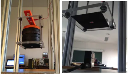
3.3. Experimental mapping - Young modulus of the SMA wire
Figure 3.2: Experimental Device.
A - 1kg weights (each)
B - Main support
C - Electrical connectors
D - SMA wire sample
E - Thermocouple
F - Leveler device
G - Weight support
H - Laser target
I - Baumer Photoelectric sensor CH-8501 Class 2 laser
J - Kaise DC power supply hy3005d
Six weights of 1kg each were placed in the weights support, allowing for an increment of stress in the wire sample. The wire sample was electrically driven by two electrical connectors linked to a power source controller and connected to a power supplier that produces an electric potential difference, causing a thermal variation in the sample. To measure the wire’s temperature in real time, a thermocouple was placed in the center of the wire sample. This thermocouple was connected to the National Instruments NI PXI-1052.
Figure 3.3: National InstrumentsNI PXI-1052 controller andkaise DC power supply hy3005d.
The National Instruments NI PXI-1052 offers advanced analog and digital signal condi-tioning, isolation, timing and synchronization features making this equipment very useful in a wide range of applications.
As it can be seen in Figure 3.4, a Baumer Photoelectric sensor CH-8501 Class 2 laser
(supplied by a kaise DC power supply hy3005d), pointing into a target positioned at the bottom side of the support for weights, was placed under the support for weights in order to record the vertical displacements experienced by the wire throughout the whole test. This laser was also connected to the National Instruments NI PXI-1052 referred above. To ensure the verticality of the load and the suitability of the readings made by the laser, a leveler device was placed at the upper face of the weight support allowing to make adjustments when placing each load increment in the wire.
3.3. Experimental mapping - Young modulus of the SMA wire
The entire experimental process was monitored by the graphical environment ofLabVIEW
(National Instruments), which comprises a PID control algorithm for the temperature of the SMA wire in real time. The wire’s temperature values read by the thermocouple, are computed into the LabVIEW platform in real time and then, through the PID algorithm, the platform is able to calculate the voltage required to apply to the SMA wire to achieve the desired temperature. As mentioned above, the heating process of the alloys is accomplished by Joule effect through the application of an electrical current. The cooling process is done by convection and therefore does not require any electric current in the wire sample.
In the LabVIEW VI two main windows can be found, one showing the lengthwise dis-placement that occurs in the wire in real time, while the other one shows the temperature of the same wire in real time as well.
3.3.2 Experimental Method
The test performed in this section approaches a typical tensile test, applying an increasing uniaxial tensile load on a specific specimen, but in this case, without reaching rupture (failure state). With this type of test, all the deformations brought into the material are uniformly distributed throughout the sample and, as the load increases in a reasonably slow speed, the tensile test allows a satisfactory measurement of the strain of the material.
All the steps performed during the experimental test are subsequently described below:
1. Initial step
First, to obtain a proper application of the load, an initial weighing of the "weights support" was performed since this one is also suspended, counting as a load to the wire. Afterwards, in order to start the experimental procedure, all components were placed together. In this initial step, the wire supported no load (except the one corresponding to the weights support) and the laser beam was directly pointed to the target. In the
LabVIEW environment, both wire temperature and strain are displayed and controlled.
2. Temperature definition
A 20oC wire temperature (more or less the room temperature) was the experiment
starting point. To achieve this temperature, the values read by the thermocouple were computed, in real time, to the LabVIEW platform and through the PID algorithm the platform was able to calculate the required voltage to be applied in the wire sample.
During the experimental test, the PID algorithm compares the value of the instantaneous temperature of the wire (read by the thermocouple) with a target temperature value previously set, calculating the error and consequently the response to be imposed to the system, in order to change the wire’s temperature. This process is repeated sequentially until the desired temperature becomes reached.
A detailed description of this Proportional-Integral-Derivative controller (PID controller) is presented in the Appendix B of this dissertation.
As 20oC was considered the room temperature, the wire length remained the same
3. Loading procedure
By adding the 1kg weight to the "weights support", the first vertical displacement value was read by the laser sensor. Knowing the initial and final length of the wire (before and after the first loading), the total deformation ratio (strain) was calculated considering:
ε= ∆L
L (3.1)
WhereL is the initial length of the wire and∆L is the value read by the laser sensor. Then, the second 1kg weight was added and new length measurements were obtained. The entire process was repeated until the maximum load (6 kg) is reached. It is impor-tant to note that according to FLEXINOLR’s catalog, 345 MPa is the maximum yield strength defined for the high temperature phase and one must not exceed this limit. As 335,7 MPa was the major stress applied to the wire during the whole experimental test, the above mentioned recommendation was fully considered.
4. Data recording
Considering a specific test temperature, all vertical displacement values were recorded (in mm) for each stress increment (in MPa), allowing to obtain a Stress Vs. Strain relation for the material, for the given temperature. It can be seen in Figure 3.5 that, as the stress in the wire increases, the strain also increases almost linearly.
y = 339,91x R² = 0,9962
0 50 100 150 200 250 300 350 400
0 0,1 0,2 0,3 0,4 0,5 0,6 0,7 0,8 0,9 1
S tr e ss ( MP a )
Strain (%)
Stress VS Strain : 20°C
Experimental Trendline
Figure 3.5: Stress - Strain curve for a 20oC temperature
Using a linear regression (see Figure 3.5), it is possible to define a representative linear function containing a particular slope value. This slope corresponds to the Young mod-ulus value of the SMA wire for the defined temperature. In this case (Figure 3.6a), the Young modulus obtained for a 20◦C wire’s temperature is Ew= 33,99 GPa.
5. Temperature definition 2
3.3. Experimental mapping - Young modulus of the SMA wire
6. Next Steps
Steps 3, 4 and 5 were consecutively repeated with temperature increments in the or-der of 10◦C, from 20oC up to a final temperature of 110oC. When dealing with this
temperature range, it is possible to ensure that the wire sample has suffered a phase transition from martensite (low temperature) to Austenite (high temperature).
3.3.3 Results
Before introducing the results of the above mentioned test, it is necessary to take into account that the accuracy of a tensile test strongly depends on the precision of the measurement devices used. With minor stress, deformation and temperature increments, it may have been possible to achieve higher precision results evaluating the stress-strain behavior of the wire sample.
The graphical results for the ten temperature values imposed to the wire are listed below.
y = 339,91x R² = 0,9962
0 50 100 150 200 250 300 350 400
0 0,1 0,2 0,3 0,4 0,5 0,6 0,7 0,8 0,9 1
S tr e ss ( MP a )
Strain (%) Stress VS Strain : 20°C
Experimental
Trendline
(a) Stress-Strain curve for 20o
C
y = 346,63x R² = 0,98648
0 50 100 150 200 250 300 350 400
0 0,1 0,2 0,3 0,4 0,5 0,6 0,7 0,8 0,9 1
S tr e ss ( MP a )
Strain (%) Stress VS Strain : 30°C
Experimental Trendline
(b) Stress-Strain curve for 30oC
y = 329,85x R² = 0,99341
0 50 100 150 200 250 300 350 400
0 0,2 0,4 0,6 0,8 1
S tr e ss ( MP a )
Strain (%) Stress VS Strain : 40°C
Experimental Trendline
(c) Stress-Strain curve for 40oC
y = 239,99x R² = 0,99077
0 50 100 150 200 250 300 350 400
0 0,2 0,4 0,6 0,8 1 1,2 1,4 1,6
S tr e ss ( MP a )
Strain (%)
Stress VS Strain : 50°C
Experimental
Trendline
(d) Stress-Strain curve for 50oC
y = 364,26x R² = 0,96169
0 50 100 150 200 250 300 350 400
0 0,1 0,2 0,3 0,4 0,5 0,6 0,7 0,8 0,9 1
S tr e ss ( MP a )
Strain (%)
Stress VS Strain : 60°C
Experimental
Trendline
(e) Stress-Strain curve for 60o
C
y = 498,51x R² = 0,97364
0 50 100 150 200 250 300 350 400
0 0,1 0,2 0,3 0,4 0,5 0,6 0,7 0,8
S
tr
e
ss (
MP
a
)
Strain (%) Stress VS Strain : 70°C
Experimental Trendline
(f) Stress-Strain curve for 70o
y = 551,35x R² = 0,98073
0 50 100 150 200 250 300 350 400
0 0,1 0,2 0,3 0,4 0,5 0,6 0,7
S
tr
e
ss (
MP
a
)
Strain (%) Stress VS Strain : 80°C
Experimental Trendline
(g) Stress-Strain curve for 80o
C
y = 510,52x R² = 0,99296
0 50 100 150 200 250 300 350 400
0 0,1 0,2 0,3 0,4 0,5 0,6 0,7 0,8
S
tr
e
ss (
MP
a
)
Strain (%) Stress VS Strain : 90°C
Experimental
Trendline
(h) Stress-Strain curve for 90o
C
y = 649,38x R² = 0,98776
0 50 100 150 200 250 300 350 400
0 0,1 0,2 0,3 0,4 0,5 0,6
S tr e ss ( MP a )
Strain (%) Stress VS Strain : 100°C
Experimental Trendline
(i) Stress-Strain curve for 100o
C
y = 587,44x R² = 0,97656
0 50 100 150 200 250 300 350 400
0 0,1 0,2 0,3 0,4 0,5 0,6 0,7
S
tr
e
ss (
MP
a
)
Strain (%) Stress VS Strain : 110°C
Experimental
Trendline
(j) Stress-Strain curve for 110o
C
Figure 3.6: Stress-Strain curves obtained for the considered temperature range.
In the previously presented graphics, one can observe a similar behavior of the wire sample regardless of the temperature to which it is subjected, where the stress-strain curve presents a linear increasing behavior throughout its whole domain.
The main difference observed between graphics is related with the slope values. This effect consolidates the increase of the modulus of elasticity for positive temperature variations.
Regarding the shape recovery force exerted by the FLEXINOL R wire, it is possible to observe (from 60◦C) a reduction in the wire’s extension (in %) when subjected to the same loads but for higher temperatures. This contraction effect can be easily noticed when the wire’s length measurements depend only on the increasing temperature (with no loading).
Table 3.1: Wire length with no loading.
Temperature Wire length T(oC) (m)
3.3. Experimental mapping - Young modulus of the SMA wire
It can be seen in the previous table (Table 3.1), that as the temperature increases, the total length of the wire sample decreases. This reduction occurs from 0,45 m to 0,43 m, which is a contraction around 4.44% (between 4 and 5%) of the initial length. This value is in accordance with the FLEXINOL R specifications mentioned in section 3.2. It is noteworthy that upon reaching 80◦C (approximately As temperature) the variation of the wire’s length (due to the increasing temperature) reaches a minimum value of 0,43 m.
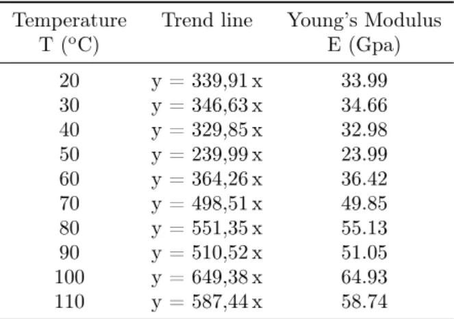
In order to summarize the evolution of the modulus of elasticity of the SMA wire in this experimental test, Table 3.2 is presented bellow. This table contains the equations of the linear regressions for each graphic of Figure 3.6 as well as the values of Young’s modulus associated to each temperature value.
Table 3.2: SMA wire Test Results
Temperature Trend line Young’s Modulus T (o
C) E (Gpa)
20 y = 339,91 x 33.99 30 y = 346,63 x 34.66 40 y = 329,85 x 32.98 50 y = 239,99 x 23.99 60 y = 364,26 x 36.42 70 y = 498,51 x 49.85 80 y = 551,35 x 55.13 90 y = 510,52 x 51.05 100 y = 649,38 x 64.93 110 y = 587,44 x 58.74
From the data of Table 3.2, it is possible to plot a scattering map, where one can observe the behavior of the modulus of elasticity as function of temperature.
0 10 20 30 40 50 60 70
0 20 40 60 80 100 120
Y o u n g Mo d u lu
s
(G
P
a
)
Temperature (ºC) Young Modulus vs. Temperature
Considered Points
Trendline
In the previous graphic (Figure 3.7), one can observe the existence of a horizontal initial baseline (between 20◦C and 60◦C), followed by an increasing line (between 60◦C and 100◦C) which turns out to horizontally stabilize after that temperature range. Looking back at the vertical axis (E), it is concluded that initially the wire presented a modulus of elasticity around 34 GPa (in martensitic phase) followed by an increase and a new stabilization of the
E values around 65 GPa (in austenitic phase).
With the proposed experimental procedure, it was possible to establish a clear relation between the Modulus of Elasticity of the SMA wire and its temperature.
For a more detailed analysis of the results for the whole experimental test, all the experi-mental data is described in the appendix A of this document.
3.4
Numerical approach - Young modulus of the SMA wire
Using the formulations presented in section 2.4, one will now implement a constitutive model, representative of the behavior of the wire sample, comprising a Kinetic Law and a Mechanical Law.
3.4.1 Kinetic law
In order to characterize the austenite phase fraction of the NiTi wire sample as function of temperature, the results from a differential scanning calorimetry (DSC) test, performed in [32] using a SETARAM-DSC92 thermal analyzer, have been taken into account. The sample, tested as received, was submitted to a thermal cycle, heated up to 130oC, held at
this temperature for 6 minutes, and then cooled to -20oC, with heating and cooling rates of
7,5oC/min. As it is referred in [32], before the DSC experiment, the sample was submitted
to a chemical etching (10 vol.% HF + 45 vol.% HNO3 + 45 vol.% H2O) in order to remove the oxide and the layer formed by the cutting operation. The results of the DSC test are presented in Figure 3.8 bellow.
3.4. Numerical approach - Young modulus of the SMA wire
The obtained DSC curve exhibits a single-step endothermic M → A transition upon heating and an exothermicA→M transition upon cooling. By considering theM →A tran-sition, due to the presence of its high peak, one can determine theAsand Af transformation temperatures, with values of about 40oC and 70oC, respectively.
With the aid of PlotDigitizer App, the DSC curve values (in mW/mg) from 39,9oC to
90oC, which was the temperature range comprising both martensite and austenite phases in
the endothermic transition (driven by heating), were extracted (see Figure 3.9).
(a) Heat Flux - PlotDigitizer analisys.
-‐0,3 -‐0,25 -‐0,2 -‐0,15 -‐0,1 -‐0,05 0 0,05 0,1
0 10 20 30 40 50 60 70 80 90 100
He
a
t
Fl u x ( m W /m g )
Temperature (ºC)
(b) Heat Flux [mW/mg].
Figure 3.9: Extraction of the Heat Flux values from the DSC curve.
According to the assumptions of chapter 2.4.2 and [47], the degree of transformation can be determined from the enthalpy of the system, expressed by the area of the DSC graphic peak. From equation (2.1) the following baseline-corrected and unsmeared DSC curve, was obtained:
-‐0,0005 0 0,0005 0,001 0,0015 0,002 0,0025
0 20 40 60 80 100 120
U n sm e a re d H e a
t
Fl u x Fu ( mW/mg)
Temperature T (ºC)
Considering the previous curve and applying the equation (2.2), one can obtain a repre-sentative curve of the austenite phase fraction f(T) as function of temperature.
-‐0,2 0 0,2 0,4 0,6 0,8 1 1,2
0 20 40 60 80 100 120
Au st e n it e P h a se Fr a c/ o n f( T) ( %)
Temperature T (ºC)
Figure 3.11: Austenite phase fraction evolution during theM →A transformation.
It is noteworthy that theAs andAf transformation temperatures stand around 40oC and 70oC respectively, just like it was presumed in the DSC run graphic.
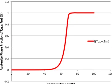
Taking into account the SMA kinetic model developed by Nikolay Zotov, Vladimir Marzynke-vitsch and Eric J. Mittemeijer [47], equation (2.3) was used to describe Figure’s 3.11 data.
-‐0,2 0 0,2 0,4 0,6 0,8 1 1,2
0 20 40 60 80 100 120
Au st e n it e P h a se Fr a c/ o n f( T, g ,v, Tm ) ( %)
Temperature T (ºC)
f(T,g,v,Tm)
Figure 3.12: Austenite phase fraction - Equation (2.3),
f(T, g, ν, Tm).
Table 3.3: Equation (2.3) fitting parameters.
Fit parameters
g ν Tm
3.4. Numerical approach - Young modulus of the SMA wire
The g and ν fitting parameters used in the equation (2.3) were chosen considering the studies of [47], with the purpose of approximating the equation (2.3) to the behavior reported in the graphic of Figure 3.11. Regarding the Tm fitting parameter, it was obtained by in-terpolation between the temperatures corresponding to the maximum transformation rate
(df /dT)max, (see Figure C.4 of Appendix C).
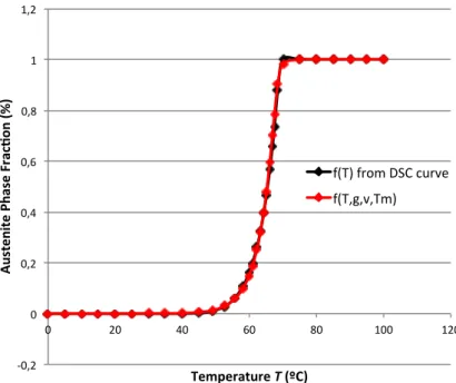
In order to verify the suitability of equation (2.3) (see Figure 3.12 ) to express the data of the Figure 3.11, a graphical overlay, represented in the Figure 3.13, was performed. It is possible to conclude that the kinetic equation (2.3) describes very well the data obtained from the DSC run.
-‐0,2 0 0,2 0,4 0,6 0,8 1 1,2
0 20 40 60 80 100 120
Au
st
e
n
it
e
P
h
a
se
Fr
a
c/
o
n
(
%)
Temperature T (ºC)
f(T) from DSC curve
f(T,g,v,Tm)