SAGE Open 1 –10
© The Author(s) 2012 DOI: 10.1177/2158244012442518 http://sgo.sagepub.com
Introduction
In recent years, mixture model has gained more and more attention among practitioners and statisticians (McLachlan & Peel, 2000). Finite mixture models (FMMs) underpin a number of statistical techniques, one of which is growth mixture modeling (GMM), a technique becoming increas-ingly popular in longitudinal studies due to its flexible analysis framework combining continuous and categorical latent variables (Bauer & Curran, 2004; B. O. Muthén, 2004; B. O. Muthén & Shedden, 1999). In a recent publication, “Handbook for Advanced Multilevel Analysis,” several researchers (B. O. Muthén & Asparouhov, 2011; Vermunt, 2011) have pointed out the importance of combining multi-level modeling with mixture models. Despite “the richness of detail that a multilevel growth mixture model can extract from the data” (B. O. Muthén & Asparouhov, 2011, p. 38), “many issues have not yet been fully resolved” due to the fact that “multilevel mixture modeling is a rather new area of sta-tistical methodology” (Vermunt, 2011, p. 78). This article attempts to examine the impact of ignoring the higher level nesting structure in multilevel mixture models (MMMs) and helps to build the body of knowledge in multilevel mixture modeling.
Despite the flexibility provided by FMM, when research-ers analyzed their data using FMM, they generally assumed that the participants were independent from each other even though it might not always be true. For example, in educa-tional setting, the data structure is very likely to contain two
or more levels (e.g., students nested within schools). Nevertheless, when researchers analyzed their data using FMM, they ignored the higher level nesting structure (i.e., schools) and analyzed the model by assuming that the stu-dents were independent from each other (e.g., D’Angiulli, Siegel, & Maggi, 2004). In a literature search we conducted in PSYCINFO (from year 2000 to 2011) for empirical stud-ies applying mixture modeling in different substantive areas, we have found only one recent study using MMM (Van Horn et al., 2008). Some of these studies did not need to use MMM because their data did not have the higher organization level. However, some studies used mixture modeling when they should have used MMM by ignoring the highest level of nesting (e.g., the school level) and mistakenly assume that individuals are independent from each other (reasons for doing so include lack of cluster ID, MMM’s model complex-ity, and/or model convergence issues). In a recent simulation study conducted by Chen, Kwok, Luo, and Willson (2010), the authors have found that when modeling latent growth tra-jectories, ignoring the highest level results in the redistribu-tion of the variance from the ignored level (i.e., the organization/school level) to the adjacent level (i.e., the
1University of North Texas, Denton, USA
Corresponding Author:
Qi Chen, Department of Educational Psychology, University of North Texas, P.O. Box 311335, Denton, TX 76203-1335, USA
Email: [email protected]
The Impact of Ignoring a Level of Nesting
Structure in Multilevel Mixture Model:
A Monte Carlo Study
Qi Chen
1Abstract
Mixture modeling has gained more attention among practitioners and statisticians in recent years. However, when researchers analyze their data using finite mixture model (FMM), some may assume that the units are independent of each other even though it may not always be the case. This article used simulation studies to examine the impact of ignoring a higher nesting structure in multilevel mixture models. Results indicate that the misspecification results in lower classification accuracy of individuals, less accurate fixed effect estimates, inflation of lower level variance estimates, and less accurate standard error estimates in each subpopulation, the latter result of which in turn affects the accuracy of tests of significance for the fixed effects. The magnitude of the intraclass correlation (ICC) coefficient has a substantial impact. The implication for applied researchers is that it is important to model the multilevel data structure in mixture modeling.
Keywords
individual/student level). The effects of ignoring clustering have not been studied in the finite mixture modeling setting. It is important to examine its impact and make applied researchers more aware of the consequences of not consider-ing the higher organization level and use caution in their interpretation of statistical results when they had to ignore a higher level.
Purpose of the Study
The purpose of this article is to examine the impact of ignor-ing a higher nestignor-ing structure in MMM on the accuracy of classification of individuals, and the accuracy as well as sta-tistical inference (i.e., Type I error rate and stasta-tistical power) of the parameters for the model of each subpopulation.
Data structure including students nested within schools is considered. Two latent classes with known group member-ships were generated and then analyzed for the true (MMM considering the higher level structure) and misspecified (FMM ignoring the higher level structure) models. Two sim-ulation studies were conducted. In Study 1, the two latent classes were balanced in both sizes and variances, whereas in Study 2, the two latent classes were unbalanced in sizes and variances. Results were presented to show how the hit rate and the relative biases (RBs) for group mean estimates and the respective standard errors were influenced by ignoring the higher level nesting structure.
Brief Review of Multilevel Mixture Models (MMMs)
In this section, key concepts related to multilevel finite (nor-mal) mixture models with continuous indicators are pre-sented. The development of MMMs drew upon two lines of research. One component of MMM is finite mixture model-ing (FMM), which assumes that the data under analysis is composed of a discrete number of components. FMM can handle situations where a single parametric family is unable to provide a satisfactory model for local variations in the observed data (McLachlan & Peel, 2000). FMM is similar to multiple group analysis; however, an important difference between mixture modeling and standard multiple group analysis is that in mixture modeling, the group membership is not observed or latent (B. O. Muthén, 2001; Vermunt & Magidson, 2005). This is why some researchers refer FMM as Finite Mixture Modeling (FMM), although statisticians often reserve the term FMM for the situation in which all response variables are categorical (Vermunt, 2007). In this article, we will use the term FMM to refer to mixture model with continuous response variables.FMM has the capacity of modeling the unknown hetero-geneous subpopulations and the random variation of the response variables within latent classes. However, FMM does not consider the situation of multilevel data in which individuals are nested within organizations. Hence, FMM cannot handle nonindependence of individuals due to cluster
sampling. As an extension to FMM, the MMMs take the nonindependence of individuals into consideration by speci-fying a model for each level of the multilevel data. The model for each level could be different, depending on whether we assume heterogeneity and/or model the random effects at the individual level and the organizational level. For example, at the individual level, we can specify a mix-ture model that models individuals’ response patterns and classifies individuals into different subpopulations as well; whereas at the organization level, we can specify a model which only models the variance of organizations, but does not classify organizations into different subpopulations. It is also possible to specify a mixture model at the organization level. However, this article only addressed the more com-mon MMM with classification at the individual level (e.g., students being classified into different subgroups within schools; patients being classified into different subtypes within clinics).
Study 1
Method
Data generation. In Study 1, data with two known sub-populations under a two-level model were first generated with equal population sizes and variances. Then, the data were analyzed as a two-level model (i.e., true model) using multilevel mixture model (MMM) and as a single-level model (i.e., misspecified model) using FMM. The two-level model for data generation is shown below:
Level 1:
Yij =β0j+β1jsubpopulationij+eij, (1a)
with
eij ~N o( ,σ ).
2
(1b)
Level 2:
β0j=γ00+µ0j, (1c)
β1j=γ01, (1d)
with
µ0j~N( ,0 τ00), (1e)
where subpopulationij was a dichotomized variable with 0 and 1 representing two different subpopulations.
50% versus 50%. Within each school, there were 20 students coming from two subpopulations, 10 at-risk versus 10 non-at-risk. Altogether, there were 800 students within each rep-lication for data generation. The number of higher level units was set to be 40 given that the recommended minimum num-ber of higher level units for MMMs is 30 (L. K. Muthén, 2003; B. O. Muthén, 2005).
In this two-level model, a total of four parameters needed to be specified: two fixed effect coefficients (i.e., γ00 and γ01) and two variances of the random effects (i.e., σ2 and τ
00). Before specifying the population parameters in the condi-tional model, a random intercept model in which there are no subpopulations is presented as follows:
Level 1:
Yij =β0j +eij
*
, (2a)
with
eij N o
*~ ( ,σ2*),
(2b)
Level 2:
β0j γ00 µ0j
* * *
= + (2c)
with
µ0 j N 0 τ0 0
* *
~ ( , ). (2d)
The variance of the random effect at Level 1 was speci-fied following Raudenbush and Liu’s (2001) criteria, namely,
σ2*=1 .
For τ00*, the intraclass correlation (ICC) formula I C C =τ σ +τ
00 2
00
( ) was used to obtain the values
corresponding to small- and medium-effect size. By fixing ICC equal to .10 as a small ICC which is very common for studies in education (Hox, 2002) and .20 as a medium ICC, the values for a small τ00* (.111) and a medium τ
00* (.250) were obtained.
According to Snijders and Bosker (1999), adding a pre-dictor (i.e., subpopulationij) at Level 1 only contributes to the variance of the Level 1 random errors but does not contribute to between-level variance. The formulas for calculating the within and between variances when there is multilevel struc-ture in the data are σ2within=σ2 and σ τ σ
2
00 2 between= +( / )n ,
where n is the number of students per school.
Using these formulae for calculation, a small (0.161) and a medium (0.300) σ2
between for the random intercept model
was obtained. After adding subpopulationij as a predictor at Level 1, ßij was actually the difference between the two sub-populations within each school (cluster), and γ01 was the average difference between these two subpopulations across all clusters. The effect size R2 was used to characterize the difference between the two subpopulations with small,
medium, and large effect sizes being 0.1, 0.3, and 0.5 according to Cohen (1988, 1992). R2= .5 meant that 50% of the variance
between the two subpopulations could be explained by their group membership. Therefore, the larger the R2, the larger the difference between the two subpopulations.
Using the R2 information, small, medium, and large ß ij
val-ues could be calculated and was 0.632, 1.095, and 1.414, respec-tively. The corresponding σ2 in the conditional model for small, medium, and high levels of group difference was 0.9, 0.7, and 0.5. τ00 for the conditional model could be solved using equation
σ2 τ σ τ σ
00 2
00 2
between= +( / )n = +( / )n
* * , because ICC
magnitude stayed the same across the random intercept and the conditional models. For ICC = .1, τ00 was 0.116, 0.126, and 0.136 for small, medium, and large effect sizes, respec-tively; for ICC = .2, τ00 was 0.255, 0.265, and 0.275 for small, medium, and large effect sizes, respectively.
After fixing γ00 to 1, the mean for Subpopulation A and the mean for Subpopulation B were calculated using Equation (1a). The mean of Subpopulation A was 1 in all conditions, and the means for Subpopulation B were 1.632, 2.095, and 2.414 at different levels of R2.
In summary, by specifying R2(0.1, 0.3, and 0.5) and ICC (.1 and .2) values, and also setting δ2 = 1, γ
00=1,the
popula-tion parameter values for the other fixed effect coefficient (i.e., γ01) and the two variances of the random effects (i.e., σ2 and τ00) were obtained.
The simulation used a 3 (effect sizes—amount of variance explained by group membership) × 2 (magnitude of ICC) fac-torial design to generate the data. A total of 500 replications were generated for each condition using SAS 9.1, yielding a total of 3,000 data sets. Each data set was then analyzed by a true model (MMM considering the higher/cluster level, type = two-level mixture) and a misspecified model (FMM ignoring the higher/cluster level, type = mixture) using Mplus 4.2 Mixture routine (L. K. Muthén & Muthén, 2006-2007).
Analysis. For each condition, valid replications for data analysis were selected because among the replications with converged results, there were latent classes with very few students (i.e., 1 or 2). A valid replication was defined as one of the two subpopulations (or classes) with class size at least equal to or larger than 6% of the total sample size (i.e., 48 out of 800). This 6% criterion was based on the average percent-age of sample size for the smallest class in published studies using FMM found in PsycINFO database.
The accuracy of classification of individuals, and the accuracy as well as the test of significance (i.e., Type I error rate and statistical power) of the parameter estimates of the model for each subpopulation were then evaluated.
Hit rate is the percentage of at-risk/non-at-risk students correctly classified as at-risk/non-at-risk. The true and mis-specified models were evaluated by comparing the hit rate difference between the two models.
replications for each of the six conditions. The RB for each parameter estimate was calculated using the following equation:
B est pop
pop
( )θ θ θ ,
θ
= −
where θest is the mean of a parameter estimate across the
valid replications and θpop is the true parameter value. RB equal to zero indicates an unbiased estimate of the parame-ter. A negative RB indicates an underestimation of the parameter (i.e., the estimated value is smaller than the true parameter value), whereas a positive RB indicates an over-estimation of the parameter (i.e., the estimated value is larger than the true parameter value). The cutoff value of 0.05 recommended by Hoogland and Boomsma (1998) was used for acceptable RB of parameter estimates.
The RB of estimated standard errors was computed using the following equation:
B S S S
S
False True
True
( ) _ _ ,
_
θ
θ θ
θ
= −
(4)
where Sθ_False is the mean of the estimated standard
errors of the group mean parameter estimate across the valid replications in the misspecified model, and
S
θ−True is thestandard deviation of the parameter estimate across the valid replications in the true model within a particular design con-dition. The standard deviation was obtained after fitting the correctly specified model to the data (i.e., the model consid-ering the higher level nesting structure), and thus represents the “true” sampling variation, or standard error, that would have been achieved had the model been properly specified. Hoogland and Boomsma (1998) recommended a cutoff value of 0.10 for acceptable RB of estimated standard errors.
ANOVAs were conducted to determine the contribution of the two design factors (i.e., R2 and ICC) and their interac-tion effect, with η2 (i.e., η2=
SSEffect SSTotal ) as the effect size indicator. η2 was used instead of the significance test because with the large number of records, the sum of square error was substantially reduced and any tiny effect could be detected as significant using the F test. Therefore, λ2 ≥.0 1 was adopted as the effect size indicator to filter out the effects trivial in magnitude and to evaluate the impact of design factors.
Results
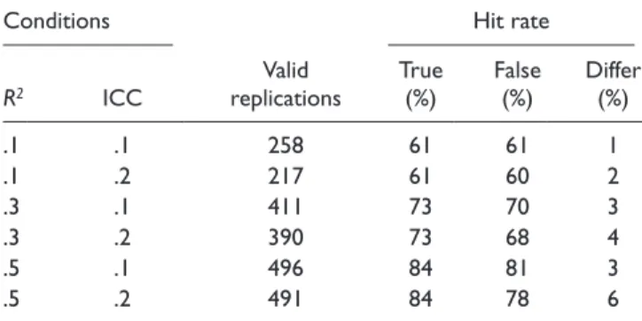
Hit rate. Table 1 presents the number of valid replications in Study 1 and the average hit rate under true and misspeci-fied models across valid replications. The results show that as group difference increased, the hit rate increased for both true and misspecified model. Besides, within the same design
condition, the hit rate under true model is always higher than that under misspecified model. As ICC increased, the differ-ence in hit rate between true and misspecified models increased.
ANOVA results indicate that only R2, F(2, 2257) = 1,2217.44; p < .001; η2 = .91, had substantial impact on the true model hit rate, which increased as R2 increased. However, for the misspecified model, both R2, F(2, 2257) = 5,904.61; p < .001; η2 = .83, and ICC, F(1, 2257) = 142.551;
p < .001; η2 = .01, had impact. The hit rate under misspeci-fied model increased as R2 increased but decreased as ICC increased. For the difference in hit rate between true and misspecified models, there was an interaction effect between
R2 and ICC, F(2, 2257) = 24.55; p < .001; η2 = .02. As R2 and
ICC increased, the difference in hit rate between true and misspecified models increased.
Relative Bias (RB) of group mean estimates. Table 2 presents the mean RB of group mean estimates across valid replica-tions under true and misspecified models. There was an underestimate of Class 1 (the smaller mean) mean and an overestimation of Class 2 (the larger mean) mean under both true and misspecified models when R2 = 1. When R2= .3 and
.5, the mean RBs under both models were close to zero, except for the mean RB for Class 1 was underestimated slightly when ICC = .2.
Table 1. Hit Rate of True and False Models in Study 1
Conditions Hit rate
R2 ICC
Valid replications
True (%)
False (%)
Differ (%)
.1 .1 258 61 61 1
.1 .2 217 61 60 2
.3 .1 411 73 70 3
.3 .2 390 73 68 4
.5 .1 496 84 81 3
.5 .2 491 84 78 6
Note: ICC = intraclass correlation; Differ = true model hit rate – false model hit rate.
Table 2. Relative Bias of Group Mean Estimates in Study 1
Conditions True False
R2 ICC Class 1 (%) Class 2 (%) Class 1 (%) Class 2 (%)
.1 .1 −23 15 −24 17
.1 .2 −23 16 −28 20
.3 .1 −5 3 −5 3
.3 .2 −6 3 −9 4
.5 .1 −2 1 0 0
.5 .2 −3 1 −1 0
Note: ICC = intraclass correlation. ˆ
ˆ ˆ
ˆ
ˆ ˆ ˆ
ˆ ˆ
ˆˆ
ˆ ˆ ˆ
Table 3. Relative Bias of Variance Estimates in Study 1
Conditions True False
R2 ICC σ2 (%) τ
00 (%) σ2 (%)
.1 .1 −20 −9 −11
.1 .2 −20 −5 0
.3 .1 −5 −16 11
.3 .2 −6 −7 26
.5 .1 −1 −16 27
.5 .2 −3 −9 53
Note: ICC = intraclass correlation.
ANOVA results showed that only R2, Fs(2, 2257) =
323.481 and 606.988; ps < .001; η2s = .22 and .35 for Class 1 and Class 2, respectively, had substantial impact on the RB of group mean estimates under true model, which decreased as R2 increased. Similar results were found for misspecified
model, Fs(2, 2257) = 366.814 and 681.945; ps < .001; η2s = .24 and .38 for Class 1 and Class 2, respectively.
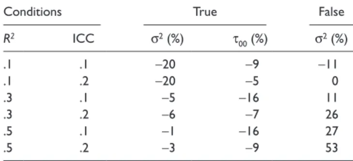
Relative Bias (RB) of variance estimates. Table 3 presents the mean RBs of variance estimates of the true and misspecified model. For the true model, the mean RB of most Level 1 and Level 2 variance estimates were within ±10%, whereas for the misspecified model, there was a trend of overestimation in Level 1 variance estimates.
ANOVA results indicated that R2, F(2, 2257) = 506.515; p
< .001; η2 = .31, had substantial impact on the RB of Level 1 variance estimates under true model, and ICC, F(1, 2257) = 32.515; p < .001; η2 = .01, had an impact on Level 2 variance estimates under true model. For the misspecified model, there was an interaction effect between R2 and ICC, F(2, 2257) = 43.726; p < .001; η2 = .014.
Relative Bias (RB) of standard errors of group mean esti-mates. Table 4 presents the mean RBs of standard errors for group mean estimates under the misspecified model. There was an inflation of standard errors for group mean estimates under the misspecified model. ANOVA results show that R2, Fs(2, 2257) = 10.017 and 13.931; ps < .001; η2s = .009 and .012 for Class 1 and Class 2, respectively, was the major source of impact when RBs of the standard errors for group mean estimates were the dependent variables.
Study 2
Method
Data generation. To extend the findings from Study 1, which was based on the balanced design (i.e., the two classes had exactly same number of observations and variance across clusters), Study 2 was conducted by taking the unbal-anced sample size and variance (i.e., unequal class size for
the two subpopulations) into account along with other design factors as considered in Study 1. There were two imbalance types, Imbalance Type 1 and Imbalance Type 2. Under Imbalance Type 1, large size was associated with large vari-ance in Group 1 and small size was associated with small size in Group 2; under Imbalance Type 2, large size was associated with small variance in Group 1 and small size was associated with large size in Group 2. The group size and variance varied at Level 1 for the two latent classes. A large group size is a group of 15 students, whereas a small group size is a group of 5 students. A larger variance group has a variance 3 times of the variance of the smaller variance group, so that the variance between the two latent groups was distinguishable. Equation (5) was used to calculate the variances of each individual group based on the size of each group. The value of S2
p, which was the pooled Level 1
vari-ance of the two latent classes, was set to be 0.9, 0.7, and 0.5, respectively, because the variance accounted for by group membership was 0.1, 0.3, and 0.5 in Study 1.
S n s n s
n n
p
2 1 1
2
2 2
2
1 2
1 1
2
= − + −
+ −
( ) ( )
(5)
The simulation used a 3 (amount of variance explained by group membership) × 2 (magnitude of ICC) × 2 (imbalance type) factorial design to generate the data. A total of 500 rep-lications were generated for each condition using SAS 9.1, yielding a total of 6,000 data sets. Each data set was then analyzed by a true model (MMM considering the higher/ cluster level) and a misspecified model (FMM ignoring the higher/cluster level) using Mplus 4.2 Mixture routine (L. K. Muthén & Muthén, 2006-2007).
Analysis. Similar to Study 1, valid replications were selected, with hit rates and RBs of parameter estimates under the 12 conditions for both true and misspecified mod-els calculated and examined. ANOVAs were conducted to determine the contribution of the design factors and all pos-sible interactions.
Table 4. Relative Bias of Standard Errors of Group Mean Estimates in Study 1
Conditions False model SE Bias
R2 ICC SE1 (%) SE2 (%)
.1 .1 9 17
.1 .2 11 8
.3 .1 20 31
.3 .2 21 20
.5 .1 3 9
.5 .2 13 13
Results
Hit rate. Table 5 presents the number of valid replications for Study 2 and the average hit rate under true and misspeci-fied models. Similar to the results found in Study 1, as group difference increased, the hit rate increased for both true and misspecified models. Besides, the hit rate under true model was always higher than that under misspecified model within the same condition. As ICC increased, the difference in hit rate between true and misspecified models increased. In addition, Imbalance Type 2 (i.e., large variance associated with small class) always had higher hit rates than Imbalance Type 1 (i.e., large variance associated with large class) when all other conditions remained the same.
ANOVA results indicated that there was an interaction effect between the magnitude of R2 and imbalance type, F(2,
3642) = 1,028.61; p < .001; η2 = .15 for true model; F(2, 3642) = 359.02; p < .001; η2 = .08 for misspecified model, for both the true and misspecified models when the hit rate was the dependent variable. The hit rate increased for both imbalance types as R2 increased. However, When R2 was
low, the difference between the two imbalance types was larger than when R2 was high. The hit rate for Imbalance
Type 2 was higher than that for Imbalance Type 1. Under the misspecified model, when other conditions stay the same, hit rate was higher when the ICC value was smaller, F(1, 3642) = 79.92; p < .001; η2 = .01.
There was an interaction effect between the magnitude of
R2 and imbalance type on the hit rate difference between true
and misspecified models, F(2, 3642) = 22.56; p < .001; η2 = .01. The estimated mean hit rate difference between true and misspecified models increased for both imbalance types as
R2 increased. Hit rate under true model was higher than that
under the misspecified model. However, at higher levels of
R2, the difference in hit rate for Imbalance Type 1 is larger
than that for Imbalance Type 2. Besides, when other condi-tions stayed the same, difference in hit rate was larger when the ICC value was larger, F(1, 3642) = 110.85; p < .001; η2 = .03.
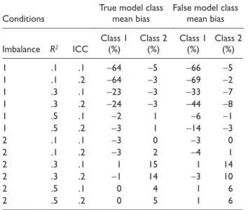
Relative Bias (RB) of group mean estimates. Table 6 presents the mean RBs of group mean estimates under true and mis-specified models. There was bias outside the range of ±10% for both the true and misspecified models. ANOVA results indicated that there was an interaction effect between R2 and ICC, Fs(2, 3642) = 449.637 and 92.023; ps < .001; η2s = .15 and .04 for the two classes in the true model; Fs(2, 3642) = 253.900 and 45.950; ps < .001, η2s = .09 and .02 for the two classes in the misspecified model, when the RBs of Class 1 and Class 2 were the dependent variables separately. The mean RB decreased for both imbalance types as R2 increased. There were more biases under Imbalance Type 1 than Imbal-ance Type 2. There tended to be more biases for Class 1 (smaller mean) mean estimate than that for Class 2 (larger mean).
Relative Bias (RB) of variance estimates. Table 7 presents the mean RBs of variance estimates of the true and misspecified model. Because the Level 1 variances for two groups were estimated separately in the true and the misspecified models, there were two σ2s for each model. For the true model, the mean RBs for Level 2 variance estimates were within or close to ±10%, and there was no η2≥.01 when RB of τ00 was the dependent variable. For Level 1 variance, there was underestimation for σ2
1 and overestimation for σ22 under Imbalance Type 1, whereas there was less biases for
Table 5. Hit Rate of True and False Models in Study 2
Conditions Average hit rate
Imbalance R2 ICC
Valid replications
True (%)
False (%)
Differ (%)
1 .1 .1 134 52 51 1
1 .1 .2 98 53 49 3
1 .3 .1 320 72 67 6
1 .3 .2 276 72 63 10
1 .5 .1 431 87 82 6
1 .5 .2 341 87 76 11
2 .1 .1 176 77 76 1
2 .1 .2 146 77 75 3
2 .3 .1 401 83 81 1
2 .3 .2 356 83 79 3
2 .5 .1 496 87 85 2
2 .5 .2 479 88 83 4
Note: ICC = intraclass correlation; Differ = true model hit rate – false model hit rate. Imbalance Type 1: Class 1—large size large variance, Class 2—small size small variance. Imbalance Type 2: Class 1—large size small variance, Class 2—small size large variance.
Table 6. Relative Bias of Group Mean Estimates in Study 2
Conditions
True model class mean bias
False model class mean bias
Imbalance R2 ICC
Class 1 (%)
Class 2 (%)
Class 1 (%)
Class 2 (%)
1 .1 .1 −64 −5 −66 −5
1 .1 .2 −64 −3 −69 −2
1 .3 .1 −23 −3 −33 −7
1 .3 .2 −24 −3 −44 −8
1 .5 .1 −2 1 −6 −1
1 .5 .2 −3 1 −14 −3
2 .1 .1 −3 0 −3 0
2 .1 .2 −3 2 −4 1
2 .3 .1 1 15 1 14
2 .3 .2 −1 14 −3 10
2 .5 .1 0 4 1 6
2 .5 .2 0 5 1 6
Note: ICC = intraclass correlation. Imbalance Type 1: Class 1—large size
Imbalance Type 2. ANOVA results indicated that there was an interaction effect between R2 and imbalance type, Fs(2, 3642) = 68.793 and 293.125; ps < .001; η2s = .035 and .126, respectively.
For the misspecified model, there was a trend of overesti-mation in σ2
2 under both imbalance types, whereas there was both underestimation and overestimation of σ2
1 only under Imbalance Type 1. ANOVA results indicated that there was an interaction effect between R2 and imbalance type, Fs(2, 3642) = 57.494 and 34.857; ps < .001; η2s = .027 and .012, respectively. In addition, ICC has a substantial impact on σ2
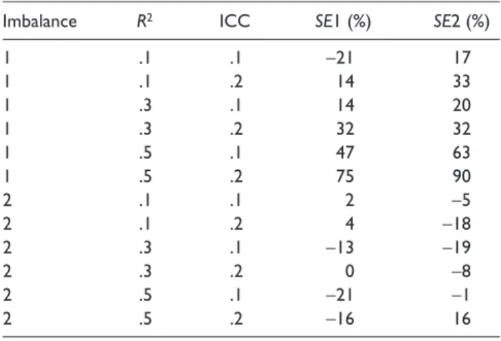
2 overestimation, F(1, 3642) = 367.945; ps < .001; η2s = .065. Relative Bias (RB) of standard errors of group mean estimates. Because the Level 1 variances were estimated separately, there were two RBs of standard errors under each model. RBs of SE1 are for the large variance groups and RBs of SE2 are for the smaller variance group under both imbalance types. Again, as shown in Table 8, there was a tendency of inflation of standard errors under the misspecified model under most conditions. ANOVA results indicated that imbalance types,
Fs(1, 3642) = 99.10 and 651.57; ps < .001; η2s = .03 and .13, and ICC, Fs(1, 3642) = 82.85 and 60.81; ps < .001; η2s = .02 and .01, were the two major contributing factors, although there was a slight interaction effect between them for SE1. The misspecified model had more inflation of standard errors under Imbalance Type 1 than Imbalance Type 2. Besides, within the same imbalance type, bias was higher at higher level of ICC.
Discussion
Study 1
When a higher level structure in cross-sectional data is ignored, the variance at the higher level is redistributed to
the lower level, thus affecting the hit rate and group mean and standard error estimates.
Hit rate. R2 is an important factor influencing hit rate. For both the true and misspecified models, hit rate increases when the R2 increases, which means that as group difference becomes larger, the classification under both models will become more accurate and this is quite reasonable.
The difference between true and misspecified model is that for true model, ICC magnitude does not affect hit rate much within the same design. Whereas for misspecified model, ICC magnitude affects the hit rate, and the hit rate is higher when ICC is smaller. Under the misspecified model, the Level 2 variance is ignored in model estimation, and more variance is ignored at higher ICC. Obviously ignoring vari-ance at Level 2 will decrease classification accuracy, and the more variance ignored, the less accurate the classification.
Relative Bias (RB) in group mean estimates. The difference in RB for group mean estimates between true and misspeci-fied models are all within ±5%, which indicates that the true and misspecified models do not differ tremendously in the estimates of the group means. In other words, there was no substantial difference on the group mean estimates between the true and misspecified models.
Relative Bias (RB) in standard error estimates. There is an inflation of standard errors for group mean estimates when a higher level nesting structure is ignored. This inflation of standard errors under the misspecified model is due to the redistribution of Level 2 variance to Level 1. When ICC is larger, misspecified model has more inflation of standard errors when all other conditions stay the same.
Study 2
After adding one more design factor—imbalance type—the findings in Study 2 related to R2 and ICC remain consistent
Table 7. Relative Bias of Variance Estimates in Study 2
Conditions True False
Imbalance R2 ICC σ2
1 (%) σ22 (%) τ00 (%) σ21 (%) σ22 (%)
1 .1 .1 −26 50 −7 −16 78
1 .1 .2 −29 47 −7 −7 110
1 .3 .1 −16 18 −12 −7 71
1 .3 .2 −16 14 −8 2 117
1 .5 .1 −2 −4 −11 17 67
1 .5 .2 −5 −3 −11 28 133
2 .1 .1 −6 −13 −11 −1 2
2 .1 .2 −7 −13 −10 2 17
2 .3 .1 −17 0 −8 −9 24
2 .3 .2 −18 −1 −5 1 43
2 .5 .1 −8 −1 −7 0 37
2 .5 .2 −9 0 −5 11 74
Note: ICC = intraclass correlation. Imbalance Type 1: Class 1—large size large variance, Class 2—small size small variance. Imbalance Type 2: Class 1—large size small variance, Class 2—small size large variance.
Table 8. Relative Bias of Standard Errors of Group Mean Estimates in Study 2
Imbalance R2 ICC SE1 (%) SE2 (%)
1 .1 .1 −21 17
1 .1 .2 14 33
1 .3 .1 14 20
1 .3 .2 32 32
1 .5 .1 47 63
1 .5 .2 75 90
2 .1 .1 2 −5
2 .1 .2 4 −18
2 .3 .1 −13 −19
2 .3 .2 0 −8
2 .5 .1 −21 −1
2 .5 .2 −16 16
Note: ICC = intraclass correlation. Imbalance Type 1: Class 1—large size
with findings in Study 1. Therefore, the following discussion focuses on the influence of imbalance type.
Hit rate. When all other conditions stay the same, the hit rate under Imbalance Type 2 is higher than that under Imbal-ance Type 1. In addition, the difference in hit rate between true and misspecified models is smaller for Imbalance Type 2, in which large group size is associated with smaller vari-ance and small group size associated with larger varivari-ance. This means that under Imbalance Type 2, the misspecified model’s performance is relatively better than the misspecified model under Imbalance Type 1. This result is not surprising because when a group has smaller variance, it is easier to identify them as coming from the same group. In Imbalance Type 2, when large size is associated with smaller variance, the participants within this group have a higher chance of being classified as the same group. Compared with Imbal-ance Type 1, where smaller group size is associated with smaller variance, although the participants within this group have a higher chance of being classified as the same group, they are still a smaller percentage of all participants compar-ing with that in Imbalance Type 2. This is why in general the Imbalance Type 2 has higher hit rates than Imbalance Type 1.
Relative Bias (RB) in group mean estimates. In general, the RBs under Imbalance Type 2 are smaller than that under Imbalance Type 1. For the same reason mentioned before, for Imbalance Type 2, it is easier for both the true and mis-specified models to classify the participants into the correct group, therefore resulting in more accurate estimate of the group mean, whereas for Imbalance Type 1, there are more RBs under different levels of R2, most likely resulting from the wrong classification of participants into wrong groups.
Relative Bias (RB) in standard error estimates. When a higher level nesting structure is ignored, the standard errors of the fixed effects (i.e., the means of the two latent classes) tend to be inflated under Imbalance Type 1 but have less bias or underestimation under Imbalance Type 2. This may result from either the misclassification of participants, or the infla-tion of Level 1 variance, or both.
Conclusion
Summary of Findings
This simulation study investigated the impact of ignoring a higher level nesting structure in multilevel mixture modeling on hit rates, the estimated latent class means, and the corre-sponding standard errors. We examined the impact of three potential factors, including the magnitude of latent class differences, the ICC between the lower and higher levels of data, and the unbalance types under the true and misspeci-fied models.
Our results indicate that first, ignoring a higher level struc-ture may result in less accurate classification of individuals to
the correct class the individual belonged to. When the vari-ance and size of the two classes in the generated samples are balanced, the true model has higher hit rates than the specified model, and the difference between true and mis-specified models is affected by group differences and the ICC. When there is unbalanced group size and variance, the true model still has higher hit rates than the misspecified model; in addition, the hit rate is higher when larger size is associated with smaller variance and smaller size is associ-ated with larger variance compared with when larger size is associated with larger variance and smaller size is associated with smaller variance.
Second, ignoring a higher level structure will result in bias in the group mean estimates for the true and misspecified models, but the difference in bias between true and misspeci-fied models is not that large. The difference between true and misspecified models is especially small when the group dif-ference is small, or when the ICC is lower, or when smaller variance is associated with larger size.
Third, ignoring a higher level structure will cause the variance at the higher level structure to be redistributed to the lower level and result in the inflation of standard errors for estimated group means, which in turn, results in an inflated Type I error rate. The inflation of standard errors is especially obvious when ICC is at a higher level or when larger variance is associated with larger size and smaller variance is associated with smaller size.
Recommendations
Limitations and Suggestions
for Future Research
In this study, we only examined the impact of ignoring a higher level structure in mixture model and only two-level structure of the data is considered. In longitudinal study, the data usually contain three levels or more (i.e., repeated measures nested within students nested within schools). In addition, the total sample size in the simulation studies was set to 800 and the cluster size was set to 20. We can change the cluster size and latent class size to see how sample size affects the hit rate and bias of parameter estimates. Another limitation is that, in real-ity, some data structure is not strictly hierarchical, they are cross-classified in the sense that students come from varied combinations of higher level nesting factors such as schools and neighborhoods. Researchers have found that ignoring the cross-classified structure will result in bias in standard error estimates although the fixed effects estimates were not affected (Luo & Kwok, 2006; Meyers & Beretvas, 2006; Van Landeghem, De Fraine, & Van Damme, 2005). However, there is no soft-ware available in the area of latent variable modeling to take into account the cross-classified structure in multilevel mixture modeling. More research and advances in software is needed for the area of multilevel mixture modeling.
Declaration of Conflicting Interests
The author(s) declared no potential conflicts of interest with respect to the research, authorship, and/or publication of this article.
Funding
The author(s) received no financial support for the research and/or authorship of this article.
References
Bauer, D. J., & Curran, P. J. (2004). The integration of continu-ous and discrete latent variable models: Potential problems and promising opportunities. Psychological Methods, 9, 3-29. Chen, Q., Kwok, O., Luo, W., & Willson, V. L. (2010). The impact
of ignoring a level of nesting structure in multilevel growth mixture models: A Monte Carlo study. Structural Equation Modeling, 17, 570-589.
Cohen, J. (1988). Statistical power analysis for the behavioral sciences (2nd Ed.). Mahwah, NJ: Erlbaum.
Cohen, J. (1992). A power primer. Psychological Bulletin, 112(1), 155-159.
D’Angiulli, A., Siegel, L. S., & Maggi, S. (2004). Literacy instruction, SES, and word-reading achievement in English-language learners and children with English as a first language: A longitudinal study.
Learning Disabilities Research & Practice, 19, 202-213.
Hoogland, J. J., & Boomsma, A. (1998). Robustness studies in covariance structure modeling. Sociological Methods & Research, 26, 329-367.
Hox, J. (2002). Multilevel analysis techniques and applications. Mahwah, NJ: Lawrence Erlbaum.
Luo, W., & Kwok, O. (2006). Impacts of ignoring a crossed fac-tor in analyzing multilevel data with cross-classified structures. Paper presented at the Annual Meeting of Psychometric Soci-ety, Montréal, Canada.
McLachlan, G., & Peel, D. (2000). Finite mixture models. New York, NY: John Wiley.
Meyers, J. L., & Beretvas, S. N. (2006). The impact of inappropri-ate modeling of cross-classified data structures. Multivariate Behavioral Research, 41, 473-497.
Moerbeek, M. (2004). The consequence of ignoring a level of nest-ing in multilevel analysis. Multivariate Behavioral Research,
39, 129-149.
Muthén, B. O. (2001). Latent variable mixture modeling. In G. A. Marcoulides & R. E. Schumacker (Eds.), New develop-ments and techniques in structural equation modeling (pp. 1-33). Mahwah, NJ: Lawrence Erlbaum.
Muthén, B. O. (2004). Latent variable analysis: Growth mix-ture modeling and related techniques for longitudinal data. In D. Kaplan (Ed.), Handbook of quantitative methodology for the social sciences (pp. 345-368). Thousand Oaks, CA: SAGE.
Muthén, B. O., & Asparouhov, T. (2011). Beyond multilevel regres-sion modeling: Multilevel analysis in a general latent variable framework. In J. J. Hox & J. K. Roberts (Eds.), Handbook for advanced multilevel analysis (pp. 15-40). New York, NY: Rout-ledge/Taylor & Francis.
Muthén, B. O. (2005). Multilevel mixture model. Retrieved from http://www.statmodel.com/discussion/messages/13/809. html?1143606816
Muthén, B. O., & Shedden, K. (1999). Finite mixture modeling with mixture outcomes using the EM algorithm. Biometrics,
55, 463-469.
Muthén, L. K. (2003). Multilevel mixture model. Retrieved from http://www.statmodel.com/discussion/messages/14/268. html?1069377168
Muthén, L. K., & Muthén, B. O. (2006-2007). Mplus user’s guide (V4.21). Los Angeles, CA: Author.
Raudenbush, S. W., & Liu, X. (2001). Effects of study duration, frequency of observation, and sample size on power in stud-ies of group differences in polynomial change. Psychological Methods, 6, 387-401.
Snijders, T., & Bosker, R. (1999). Multilevel analysis. Thousand Oaks, CA: SAGE.
Van Horn, M. L., Fagan, A. A., Jaki, T., Brown, E. C., Hawkins, J. D., Arthur, M. W., & Catalano, R. F. (2008). Using multilevel mix-tures to evaluate intervention effects in group randomized trials.
Multivariate Behavioral Research, 43, 289-326.
Vermunt, J. K. (2007). Latent class and finite mixture models for multilevel data sets. Statistical methods in medical research. Retrieved from http://spitswww.uvt.nl/~vermunt/
Vermunt, J. K. (2011). Mixture models for multilevel data sets. In J. J. Hox and J. K. Roberts (Eds.), Handbook for advanced mul-tilevel analysis (pp. 59-81). New York, NY: Routledge/Taylor & Francis.
Vermunt, J. K., & Magidson, J. (2005). Structural equation models: Mixture models. In B. Everitt & D. Howell (Eds.), Encyclope-dia of statistics in behavioral science (pp. 1922-1927). Chichester, UK: Wiley.
Bios