The Measurement and Inclusion of a Stochastic
Ore-Grade Uncertainty in Mine Valuations Using
PDEs
G.W. Evatt
∗P.V. Johnson
†P.W. Duck
‡S.D. Howell
§Abstract—Mining companies world-wide are faced with the problem of how to accurately value and plan extraction projects subject to uncertainty in both fu-ture price and ore grade. Whilst the methodology of modelling price uncertainty is reasonably well un-derstood, modelling ore-grade uncertainty is a much harder problem to formulate, and when attempts have been made the solutions have taken unfeasibly long times to compute. This paper provides a new partial differential equations approach to the problem, and achieves this by treating the grade uncertainty as a stochastic variable in the amount extracted from the resource. We show that this method is well-posed, since it can realistically reflect the geology of the sit-uation, and in addition it enables solutions to be de-rived in the order of a few seconds. The paper also provides for ore-grade parameter estimation by us-ing Maximum Likelihood Estimates on the estimated ore-grade data set, thus generalising the approach. A comparison is made between a real mine valua-tion where the prior estimate of ore grade variavalua-tion is taken as fact, and our approach, where we treat it as a stochastic uncertain estimate.
Keywords: Real-Options, Ore-Grade Uncertainty, Stochastic Control, Reserve Valuations, Mining.
1
Introduction
The planning of an extraction project and its associ-ated valuation is exposed to many uncertainties. A project can last for many years, and is therefore subject to wide variations in the underlying commodity price. It is also subject to variation in the grade or quality of ore, whose expectations are estimated by interpolat-ing between pre-extraction bore-holes. This interpola-tion, known as Kriging, produces estimation errors, even though subsequent mine planning treats the Kriging
es-∗[email protected]. School of Mathematics,
Uni-versity of Manchester. This work was helped by Gemcom Software International, and funded by the SPRIng project of the Engineering and Physical Sciences Research Council, UK
†[email protected]. School of
Mathemat-ics, University of Manchester.
‡[email protected]. School of Mathematics,
Uni-versity of Manchester.
§[email protected]. Manchester University Business
School.
timates as fact. The traditional, and most widely-used application of Kriging within numerical-based mine plan-ning, is in the Lerchs-Grossmann algorithm [12] which is an extremely useful method for devising an optimal mine design. This involves taking the estimated orebody model, which consists of a large number of constituent blocks, and then designating which blocks should be ex-tracted so as to maximise the mines value. However, the Lerchs-Grossman algorithm does not take account of price uncertainty, grade uncertainty, or discount rates [19], and therefore current mine valuations and planning do not properly address these important uncertainties. As such a new approach is required to incorporate grade and price uncertainty into mine valuations and planning.
Whilst there is general agreement that the commodity price can be modelled as a exogenous stochastic pro-cess [1], [18], there appears to be no agreed method for modelling grade uncertainty. Recent attempts have fo-cused upon planning for plausible simulated ore-bodies using mixed integer programming (MIP), where multiple ore-bodies are generated in a Monte-Carlo-type fashion [10], [14], [17], or using genetic algorithms [15]. Once a particular ore-body has been generated, numerous paths through the mine are calculated, where each path carries its own valuation, which in turn is calculated from nu-merous price simulations. It is clear that this approach involves an extremely large number of simulations. Find-ing an approximately optimal valuation and schedule can involve computational times of nearly twenty-four hours [4], even for mines with fewer than the 106 blocks which
are common, making MIPs unfeasible for common usage for large mines. Although this approach does have its merits, it is rare to find a robust defense of which param-eters behind the geological uncertainty were used, and how such methods for determining parameter estimates can be made general to all mines. In the oil and gas in-dustry, early stage research has recently been conducted to quantify, and utilise, the geological uncertainty from explorative bore-holes, where improved estimates upon geological measurements are obtained [9].
simula-tions approaches. We achieve this via partial differential equations (PDEs), as originally suggested in [8]. This form of modelling extends existing PDE mine valuation methodologies which have not considered grade uncer-tainty [3], [7], [11]. The advantage of PDEs, is that one can extract either close form solutions from them, nu-merical solutions, or approximations to them. This then allows one to gain rapid insight into the core dynamics and governing processes underpinning a system. Approx-imate solutions also, crucially, allows one to robustly test numerical solutions, so that one can test the reliability of numerical codes. This use of PDEs not only gives far faster computational speeds, allowing rapid calculation of model sensitivities but also allows several classes of opti-mal decisions to be incorporated, as demonstrated in [11] and [7].
In Section 2 we propose to model the grade quality as a stochastic uncertainty, where the stochastic behavior is realised as one extracts ore from the mine; a higher ex-traction rate implies the grade uncertainty will fluctuate faster. As shown in Section 3, this method can model a mine in a continuum manner using partial differential equations (PDEs). This formulation allows for model be-havior to be investigated and, as shown in Section 4, in some instances it allows for exact solutions to be derived. In Section 5 we present results for a particular single-ore mine, composed of some 20,000 blocks.
2
Data Interpretation
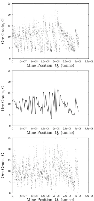
Our sample grade data for the weight of resource per unit of estimated ore extracted, G (grams per tonne), is from a sample mine composed of 30,000 blocks, and the order of extraction has been specified1. By
view-ing this data in order of extraction, Figure 1 (top), one can see howGvaries through the cumulative amount ex-tracted, ¯Q. However, given that measurement error exists at each data point, we interpret this sample of data as one random simulation from a whole range of possible Kriging samples, where each simulation will lie closely around a specified mean-path. This mean-path could be regarded as an interpolation between the known data-points (which themselves are functions of measurement error). To model this large range of random simulations, we treat the grade variation as a stochastic random pro-cess through ¯Q. A suitable model is a CIR process [6] of the form,
dG=k(α( ¯Q)−G)dQ¯+σG √
GdXG, (1)
whereα( ¯Q) is the mean-path ofGthrough the ore-body (its spatial pattern being given), and dXG, is normally
distributed as N(0,pdQ¯). This process allows the re-alised ore grade to vary either side of the estimated mean-path, but without the grade becoming less than zero.
1The data has been supplied by Gemcom Software International,
a large mining industry solutions provider.
This model is easy to generalise, for example to include Levy processes, which we leave for future work.
We next need to estimate the associated parameter val-ues of k, σG and α( ¯Q). The mean value α is relatively
straight-forward to generate; we create this using a cubic spline interpolated from Kriged data and is shown in Fig-ure 1 (centre). This gives us a smooth mean-path for ore grade variation. For the remaining two parameters we compute infill maximum likelihood estimates for a CIR process (eq. 71 and 72, [16]). Using these equations on our data estimates the parameter values to be
k= 52 kg−1 and σ
G= 9.6 G1/2 kg−1/2. (2)
To show how these parameter estimates behave, Figure 1 (bottom) shows one particular simulation using these pa-rameter values, SDE and mean-path. As it demonstrates, the simulation is qualitatively consistent and representa-tive of the data, consequently we view this methodology well-posed. In Section 5 we compare a valuation assum-ing this level of grade uncertainty with a valuation which treats the input Kriging data as fact.
It may be the case that the mining company already has knowledge to the uncertainty surrounding the grade es-timates (see [13] for an example). It is feasible that one could use these (appropriately transformed) parameter values into 1, provided the uncertainty is Gaussian. This then allows the user to harness the power of a PDE ap-proach, without having to use the alternative parameter estimates given by .
3
Model Construction
To create a finite-reserve valuation, V, we can choose to utilise one of two methods to arrive at the same un-derlying equation. The first method is the standard in financial mathematics, known as acontingent claims ap-proach. This relies upon being able to constructing a risk-neutral portfolio containing the mine valuation and other suitable traded assets, as originally explained by [2]. The second method is by utilising the Feynman-Kac method probabilistic approach. This method relies upon being able to take expectations, and is fully explained in [7], in relation to calculating the expected lifetime of an extraction project. In this current paper, we shall explain how the first, contingent claims, approach can be used.
We first prescribe four state-space variables. These are the priceSper unit of the underlying resource in the ore, the cumulative weight of ore extracted from the mine
¯
Q, time t and resource ore grade G. However, to aid notational consistency, we use the variable for remaining resource,Q, defined by,
0 5 10 15 20 25
0 5e+07 1e+08 1.5e+08 2e+08 2.5e+08 3e+08 3.5e+08
O
re
G
ra
d
e,
G
Mine Position, Q, (tonne)
0 5 10 15 20 25
0 5e+07 1e+08 1.5e+08 2e+08 2.5e+08 3e+08 3.5e+08
O
re
G
ra
d
e,
G
Mine Position, Q, (tonne)
0 5 10 15 20 25
0 5e+07 1e+08 1.5e+08 2e+08 2.5e+08 3e+08 3.5e+08
O
re
G
ra
d
e,
G
Mine Position, Q, (tonne)
Figure 1: The top figure shows ore-grade data from a sample mine (supplied by Gemcom Software Interna-tional), the middle graph shows its mean path and the third graph shows a grade simulation generated from equation (1) using the mean-path and the parameter val-ues from (2).
where Qmax is the maximum ore quantity extractable
from the reserve. An obvious consequence of this is that
dQ = −dQ¯. With this, the rate of extraction of
ore-bearing material,q, is introduced via the equation
dQ=−qdt, (4)
and will be subject to physical and practical constraints on its maximum and minimum levels, requiring q ∈
[qmin, qmax]. This is not to say that q is a continuous
function, as mine operations often work in a on/off (bang-bang) fashion, where switching between on and off states is costly.
We maintain the use of a CIR process to describe the grade uncertainty as given by equation (1), and without loss of generality we assume the underlying price S to follow a geometric Brownian motion,
dS=µSdt+σsSdXs, (5)
whereµis the drift andσsthe volatility ofS. The random
variabledXs, is normally distributed asN(0, √
dt).
Using this notation, we may apply Ito’s lemma to write an incremental change in V as,
dV =σs∂V
∂SdXs+σG √
G∂V
∂GdXG (6)
+ ∂V
∂t +
1 2σs
2∂2V ∂S2 +µ
∂V ∂S
dt
−
−∂V∂Q+12GσG2∂ 2V
∂G2+k(α−G) ∂V ∂G
dQ,
where we have taken powers of (dt)2 and (dQ)2 to be
negligible. We wish to remove thedQterm via equation (4), which means that equation (6) can be transformed into,
dV =σ1 ∂V
∂SdXs+σG √
G∂V
∂GdXG (7)
+
∂V ∂t −q
∂V ∂Q+
1 2σ1
2∂2V ∂S2 +µ
∂V ∂S
dt
+ 1
2qGσG
2∂2V
∂G2+qk(α−G) ∂V ∂G
dt.
To follow the conventional approach in creating and valu-ing risk-free portfolios, we construct a portfolio, Π, in which we are instantaneously long in (owning) the mine and are short in (owing) γs amounts of commodity
fu-tures contracts and short in γG amounts of options on
the mine C (this option could be a call or put option, just so long as it is an option on the same mine). This defines Π =V −γsS−γGC, such that,
dΠ =dV −γsdS−γGdC. (8)
This portfolio is designed to contain enough freedom in
γsandγGto be able to continually hedge away the
uncer-tainties ofdXsanddXG, which is the standard approach
in creating risk-free portfolios [18], [20]. It also means that within a small time increment, dt, the value of Π will increase by the risk-free rate of interest minus any as-sociated economic value generated during the increment. This economic value is typically composed of two parts, the first, negative, being the cost per unit to extract ore,
ǫM, and the second, positive, the cash generated by
stage of processing (e.g. milling) is usually required after ore extraction to isolate a saleable form of the resource. We model the case where the processing cost is variable and avoidable, so processing is done if qSG > ǫP, where ǫP is the processing cost per unit of ore extracted. With
this form of optimal decision the incremental change in portfolio value may be written as
dΠ =rΠdt−γSδSdt−max(0, qGS−ǫP)dt−ǫMdt. (9)
By using appropriate values ofγsandγG to be,
γs= ∂V ∂S −
∂V ∂G
∂C
∂G
−1∂C
∂S,
γG= ∂V ∂G
∂C
∂G
−1
, (10)
and substituting equations (5), (7) and (8) into (9), we may write our two-factor valuation equation as,
1 2σs
2S2∂2V ∂S2 +
1 2qGσG
2∂2V ∂G2 +
∂V ∂t −q
∂V
∂Q (11)
+ (r−δ)S∂V
∂S +qk(ˆα−δ) ∂V ∂G −rV + max(0, qGS−ǫP)−ǫM = 0,
where ˆα =α−σGλG/κ, and λG is the market price of
risk for ore grade. If we wish to reduce this model to a one-factor model, with price as the only uncertainty, we can set the grade quality to be a constant, giving,
∂V ∂t −q
∂V
∂Q+ (r−δ)S ∂V ∂S +
1 2σs
2S2∂2V
∂S2 (12)
−rV + max(0, qGS−ǫP)−ǫM = 0.
This is the standard one-factor equation of Brennan and Schwartz (eq. 15, [3]), except that they added taxation terms.
We next need to prescribe boundary conditions for (11). The boundary condition that no more profit is possible occurs either when the reserve is exhausted Q = 0, or when a lease to operate the mine has reached its expiry datet=T, hence:
V = 0 on Q= 0, or t=T. (13)
Since the extraction rate will have a physical upper bound, the extraction rate and cost will not vary with
S when S is large. This permits a far field valuation of the form,
∂V
∂S →A(G, Q, t) as S→ ∞. (14)
When the underlying resource price is zero we need only solve the reduced form of equation (11) withS= 0.
The boundary conditions on G are that its behavior is convection-dominated as it moves far from above its mean
or tends to zero, since diffusion effects are then negligi-ble. In these cases we solve equation (11) without second derivatives of G. Hence G is unlikely to drift far from its mean, as is standard with mean-reverting processes. Specifically, the conditions become,
−∂V ∂τ −q
∂V ∂Q+qκα
∂V
∂G+ (r−d)S ∂V ∂S
+1 2σ
2
SS2
∂2V
∂S2 −rV −ǫM = 0, (15)
as G→0, and as G→ ∞we require,
−∂V∂τ −q∂V∂Q+qκ(α−G)∂V∂G+ (r−d)S∂V∂S
+1 2σ
2
SS2
∂2V
∂S2 −rV +qGS−ǫP−ǫM = 0. (16)
This complete the specification of our underlying euqa-tion and its boundary condieuqa-tions, and we are now in a position to conduct an analysis upon deriving solutions from it.
4
Reserve- and Time- Dependent
Ex-traction Rate
In this section we simplify to assume that the rate of extraction and the decision to process are independent of both price and ore grade. This simplifies the extraction rate and the extraction-processing cost per unit of ore respectively to the forms q = q(Q, t) and ǫ = ǫ(Q, t). Hence the cash flows generated by the mine are of the formqSG−ǫ, since there is no longer a decision whether
or not to process. Using this and the fact that dQ/dt=
−q, we may determine Q(t) exactly, and calculate the
moment when the reserve will be exhausted, T. There are two alternative ways of defining T; first as the lease contract expiry date, and the other as the date when the extractable amount of reserve is exhausted. If these dates differ, one would take T as the lesser of the two. These assumptions allow us to remove theQvariation from our model, and write ¯q(t) =q(Q(t), t) and ¯ǫ(t) =ǫ(Q(t), t).
We begin by searching for a solution to (11), as suggested by (14), with theQderivative no longer necessary, of the form,
V =SV1(G, t) +V2(G, t). (17)
By substituting this into equation (11) we obtain the two equations,
∂V1
∂τ −qκ¯ (ˆα−G) ∂V1
∂G −q¯
1 2σ
2
GG
∂2V 1
∂G2 +dV1=Gq,¯ ∂V2
∂τ −qκ¯ (ˆα−G) ∂V2
∂G −q¯
1 2σ
2
GG
∂2V 2
∂G2 +rV2+ ¯ǫ= 0.(18)
We may split equation (18) up further to seek a solution of the formV1(G, τ) =φ(τ)G+ψ(τ), such that,
φ′+ (¯qκ+δ)φ= ¯q,
By introducing the variable ξ(τ) = Rτ
0 q(x)dx, we may
write our solution forφ, ψandV2 as,
φ=e−(κξ+δτ)Z τ
0
q(η)eκξ(η)+δηdη,
ψ=e−dτZ τ 0
καq(η)φ(η)eδηdη,
V2=−e−rτ
Z τ
0
ǫ(η)erηdη. (20)
In the particular case of a constant extraction regime, these integrals can be calculated to be,
¯
φ=qκ¯q¯+d 1−e−(¯qκ+d)τ,
¯
ψ= qqκ¯¯2κα+δn1
d 1−e−
δτ
+ 1 ¯
qκ e−
(¯qκ+d)τ
−e−δτ
o
,
V2= ǫr¯(1−e−rτ), (21)
which determines our exact solution to a mine valuation in the presence of price and ore-grade uncertainty, when extraction and processing are independent of price and grade.
5
Price Dependent Extraction Rates
Let us return to the more general case where we oper-ate a processing constraint, equation (11). Since we can no longer predict a date T when the mines value will be exhausted, we must retain all derivatives within the model and turn to numerical techniques for solution. As detailed in [8] and [5], we choose to solve (11) using a semi-Lagrangian scheme, in which the solution is evalu-ated on the characteristics dQ = −qdt via an
interpo-lation between the adjacent nodes. This scheme can be second-order convergent in time and thus allows for ac-curate solutions to be quickly derived.
5.1
Example Valuation
We compare valuations of a single ore sample mine (as detailed in Section 2), where one valuation assumes error of (and around) the Kriging estimate or ore grade, and the other takes that estimate as fact. This is equivalent to comparing a valuation made with all possible ore-grade simulations to a valuation made with just ore-grade sim-ulation. For the grade uncertainty we use the inferred parameter values of (2) and the mean-path of the grade as shown in Figure 1 (middle), and take our other price parameter values to be,
σS = 0.5 yr−1/2, r= 0.1 yr−1, δ= 0.1 yr−1. (22)
For the mine extraction cost parameters we use ǫM =
$1 tonne−1 and ǫ
P = $4 tonne−1, and the processing
capacity constraint of ore-bearing tonnage is qmax =
20,000,000 tonne yr−1, as specified by Gemcom
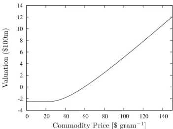
Soft-ware International. With these we are able to construct our price and grade uncertainty valuation as shown by
-4 -2 0 2 4 6 8 10 12 14
0 20 40 60 80 100 120 140
Commodity Price [$ gram−1]
V
a
lu
a
tio
n
($
1
0
0
m
)
Figure 2: Valuation of a mine reserve for differing lev-els of current commodity price made in the presence of stochastic grade uncertainty.
Figure 2. As expected the valuation becomes linear in
S for higher prices, and losses are limited for low prices (roughlyS <30 $ gr−1). This is expected, as we are
op-erating a processing decision rule where we only process cost-effective ore.
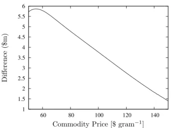
To compare this valuation under both price and grade un-certainty with one where there is only price unun-certainty, Figure 3 shows the difference between these valuations for a range of prices. At higher prices, grade uncertainty has only a small impact on the valuation. This might be ex-pected, as the expected benefits of unexpectedly high ore grade are symmetrical with the losses of its unexpectedly low grade. The only region where these opposing effects do not cancel each other out, is when the expected cash from sales is similar to the cost of processing. Here the mine has a valuable option to process all or none of the current flow of extracted material, avoiding processing where it is unprofitable. This explains the existence of a maximum point in Figure 3.
6
Conclusions
1 1.5 2 2.5 3 3.5 4 4.5 5 5.5 6
60 80 100 120 140
Commodity Price [$ gram−1]
D
iff
er
en
ce
($
m
)
Figure 3: The difference between valuations where one treats the ore-grade as an uncertainty and the other where one treats it as fact, for a range of underlying prices. This is equivalent to viewing the difference be-tween a valuation made with all possible ore-grade simu-lations, to a valuation made with just one simulation.
the CIR process could be made, such as the inclusion of jumps, the underlying methodology of the paper would remain the same.
We find for our example mine, that including price and ore grade uncertainty adds up to five million dollars to a valuation assuming only price uncertainty. At high levels of the commodity price, the option not to process poorer grades of ore is seldom used and adds relatively little value, but at lower commodity prices, and higher levels of ore grade volatility, this option appreciably raises the mines value.
It is hoped that this paper also raises the issue that research which includes an ore-grade uncertainty, must demonstrate open and defensible techniques for defining ore-grade uncertainty parameter values. This will enable practitioners and scientists alike, to improve this field of research at a much faster pace, as appears to be the case in oil and gas exploration, [9].
References
[1] Black, F., The Pricing of Commodity Contracts, Journal of Financial Economics, 3, pp. 167–179, 1976.
[2] Black, F., and Scholes, M.J.The pricing of options and corporate liabilities, Journal of Political Econ-omy, 81, pp. 637–659, 1973.
[3] Brennan, M.J., and Schwartz, E.S.,Evaluating Nat-ural Resource Investments, The Journal of Business, 58, 2, pp. 135–157, 1985.
[4] Caccetta, L., and Hill, S.P., An Application of Branch and Cut to Open Pit Mine Scheduling, Jour-nal of Global Optimisation, 27, pp. 349–365, 2003.
[5] Chen, Z., and Forsyth, P.A.,A semi-Lagrangian Ap-proach for Natural Gas Storage Valuation and Op-timal Operation, Siam J. Sci. Comput., 30, 1, pp. 339–368, 2007.
[6] Cox, J.C., Ingersoll, J.E., and Ross, S.A.,A theory of Term Structure in Interest Rates, Econometrica., 53, 2, pp. 385–407, 1985.
[7] Evatt, G.W., Johnson, P.V., Duck, P.W., Howell, S.D. and Moriarty, J. The Expected Lifetime of an Extraction Project, Proceedings of the Royal Society A, Firstcite, 2010. doi: 10.1098/rspa.2010.0247
[8] Evatt, G.W., Johnson, P.V., Duck, P.W., and How-ell, S.D. Mine Valuations in the Presence of a Stochastic Ore-Grade, Lecture Notes in Engineering and Computer Science: Proceedings of The World Congress on Engineering 2010, WCE 2010, 30 June -2 July, -2010, London, U.K., III, pp.1811-1866, -2010.
[9] Farmer, C.L., Fowkes, J.M., and Gould, N.I.M. Op-timal Well Placement, ECMOR XII 12th European Conference on the Mathematics of Oil Recovery, 6-9th September, Oxford, U.K., B033, 2010.
[10] Jewbali, A., and Dimitrakopoulos, R., Stochastic Mine Planning - Example and Value from Integrat-ing Long- and Short-Term Mine PlannIntegrat-ing Through Simulated Grade Control, Orebody Modelling and Strategic Mine Planning, The Australasian Institute of Mining and Metallurgy, Melbourne, second edi-tion, pp. 327–333, 2009.
[11] Johnson, P.V., Evatt, G.W., Duck, P.W., and How-ell, S.D. The Derivation and Impact of an Optimal Cut-Off Grade Regime Upon Mine Valuation, Lec-ture Notes in Engineering and Computer Science: Proceedings of The World Congress on Engineering 2010, WCE 2010, 30 June - 2 July, 2010, London, U.K., pp. 358-364, 2010
[12] Lerchs, H., and Grossmann, I.F.,Optimal Design of Open Pit Mines, Cana. Inst. Mining Bull, 58, pp. 47–54, 1965.
[13] Li, S., Dimitrakopoulos, R., Scott, J. and Dunn, D.
Quantification of Geological Uncertainty and Risk Using Stochastic Simulation and Applications in the Coal Mining Industry, Orebody Modelling and Strategic Mine Planning, The Australasian Institute of Mining and Metallurgy, Perth, 22-24 November, pp. 185–191, 2004.
Strategic Mine Planning, The Australasian Institute of Mining and Metallurgy, Melbourne, second edi-tion, pp. 225–234, 2009.
[15] Myburgh, C. and Deb, K. (2010). Evolutionary Al-gorithms in Large-Scale Open Pit Mine Scheduling,
Proceedings of the 12th annual conference on Genetic and evolutionary computation:1155–1162.
[16] Phillips, C., B., and Yu, J.,Maximum Likelihood and Gaussian Estimation of Continuous Time Models in Finance, Handbook of Financial Time Series, T.G. Anderson et. al., Springer-Verlag, pp. 497–530, 2009.
[17] Ramazan, S., and Dimitrakopoulos, R., Stochastic Optimisation of Long-Term Production Scheduling for Open Pit Mines with a New Integer Programming Formulation, Orebody Modelling and Strategic Mine Planning, The Australasian Institute of Mining and Metallurgy, Melbourne, second edition, pp. 385–391, 2007.
[18] Schwartz, E.S., The Stochastic Behavior of Com-modity Prices: Implications for Valuation and Hedg-ing, The Journal of Finance, LII, 3, pp. 923–973, 1997.
[19] Tolwinski, B., and Underwood, R.,A Scheduling Al-gorithm for Open Pit Mines, IMA Journal of Mathe-matics Applied in Business and Industry, 7, pp. 247– 270, 1996.