Ambient. constr. vol.17 número3

(1)

KRÜGER, E. L.; FERNANDES, L.; CARDOSO, G. T.; KAVAMURA, E. E. Proposition of a simplified method for predicting 57

predicting hourly indoor temperatures in test

cells

Proposta de um método simplificado de predição de

temperaturas internas horárias em células-teste

Eduardo Leite Krüger

Leandro Fernandes

Grace Tibério Cardoso

Emilio Eiji Kavamura

Abstract

est cells can be used for testing the thermal performance of different passive systems and building components. Predictive methods for estimating indoor air temperatures can further enhance the number of configurations tested without increasing the amount of test cells to be built. Thus, direct comparisons can be drawn for identical background climatic conditions. In its most basic form, formulas are generated by linear regression from relatively short data sets, which provide daily indoor temperature conditions. However, for more detailed analyses, daily indoor temperature predictions may not suffice. In this paper, a method for obtaining hourly indoor air temperature predictions is proposed. It is based on rising and decreasing rates of the indoor temperature fluctuation relative to outdoors, which translates to warming or cooling trends of indoor thermal conditions. The applicability of the method is for test cells. It is a simple method yet capable of predicting the thermal behavior of complex physical processes. The method was tested using measured data from experiments in a test cell, built with conventional building materials in Brazil. Results showed high performance with mean bias of 0.27 °C to measured data and Pearson’s r 0.99. When compared to traditional regression-based models, the method proposed showed better results.

Keywords: Indoor temperature predictions. Thermal performance. Test cells.

Resumo

Células-teste permitem testar o desempenho térmico de diferentes sistemas de condicionamento térmico passivo e componentes de construção. O uso de métodos preditivos para estimar temperaturas do ar internas pode ampliar o número de configurações testadas sem aumentar a quantidade de células a serem construídas. Dessa forma, podem ser realizadas comparações diretas para condições climáticas idênticas. Em sua forma mais básica, as fórmulas são geradas por regressão linear a partir de conjuntos de dados relativamente curtos, os quais fornecem condições diárias estimadas. Contudo, em análises mais detalhadas, a estimativa diária da temperatura interna pode não ser suficiente. Neste trabalho é proposto um método para a obtenção de estimativas horárias de temperatura do ar interna, o qual se baseia no uso de um fator majorador ou redutor de alterações na temperatura interna em relação à externa, o qual reflete uma tendência de aquecimento ou de resfriamento das condições térmicas internas. A aplicabilidade do método é para células-teste. Trata-se de um método simples, porém capaz de predizer o comportamento térmico de processos termofísicos complexos. O método foi testado a partir de dados experimentais de uma célula-teste construída com materiais de construção convencionais no Brasil. Os resultados mostraram alto desempenho com erro médio de 0,27 °C para os dados medidos e correlação de Pearson de 0,99. Quando comparado a modelos de regressão, o método proposto apresenta resultados superiores.

Palavras-chave: Estimativa de temperaturas internas. Desempenho térmico. Células-teste.

T

Eduardo Leite Krüger

Universidade Tecnológica Federal do Paraná Curitiba – PR – Brasil

Leandro Fernandes

Universidade Federal do Paraná Curitiba – PR – Brasil

Grace Tibério Cardoso

Faculdade Meridional IMED Passo Fundo – RS – Brasil

Emilio Eiji Kavamura

Universidade Federal do Paraná Curitiba – PR – Brasil

(2)

Introduction

Among the many methods to evaluate building materials and passive design strategies are naturally-exposed test cells. These cells are compact buildings designed for experimental purposes with some features of actual buildings. Thus, low-cost analyses can be performed in a simplified object, which can be designed in such a way that only relevant components are tested at a time in controlled experiments (HITCHIN, 1993). Test cells are also an alternative when conventional building prototypes are not available for testing (STRACHAN; BAKER, 2008).

In contrast with laboratory-based experiments, where experimental conditions are stationary, open-air test cells can be tested dynamically, which brings advantages in more variable, tropical climate conditions (as opposed to winter conditions in temperate climate regions). According to Strachan and Baker (2008), test cells can fill the gap between steady-state, lab-based experiments and those conducted in conventional buildings. In field studies supported by test cells, there is usually a control cell which is compared to one or more experimental cells. Naturally, the larger the amount of cells to be tested, the higher the costs involved. Consequently, opting for a reduced amount of test cells can lower the overall research budget. In this case, using predictive formulas is advantageous and allows for inter-comparisons between different components and/or operation modes for the same period of analysis.

The subject of indoor temperature predictions (average, minimum and maximum) from outdoor climatic parameters and thermo-physical properties of building materials comprising the building envelope was firstly introduced by Givoni (1976) in the second edition of Man, Climate and Architecture. This predictive method is called the ‘Response Factor Method’ and was developed for multi-layer building elements under transient exposure conditions to predict indoor temperatures. Similarly, the ‘Total Thermal Time Constant Method’, developed by Hoffman and Givoni (1973), calculates the indoor air temperature response to cyclic variations of outdoor temperatures and external surfaces.

At a later stage, from monitored summer data in two unoccupied dwellings in Pala, South California, Givoni (1999) developed predictive formulas, which related daily indoor minimum and maximum temperatures to outdoor climatic factors. The constants in these formulas were specific to the monitored buildings, despite not taking into account thermo-physical features of the building envelope. Constants in the formulas reflect the so-called

‘thermal signature’ of the monitored building and are specific to a given building, according to an operation mode or to a particular configuration of the passive system to be tested.

Givoni and Vecchia (2001) used multivariate linear regression to describe the daily indoor average, minimum and maximum temperatures from outdoor measurements in occupied houses in Descalvado, Brazil. They found that indoor temperatures could be predicted exclusively from the outdoor average, minimum and maximum temperatures. A further application of the same method was tested in a larger sample of 18 low-cost dwellings in Curitiba, Brazil, which had been previously monitored by Krüger and Dumke (2001). Daily indoor temperature predictions were compared to computer simulation results with a more significant match to measured data than the latter (KRÜGER; GIVONI, 2004). Various tests were additionally carried out, for example to include thermo-physical parameters to enhance the predictive potential of the formulas (GIVONI; KRÜGER, 2003).

The applicability of the predictive method for the indoor average, minimum and maximum air temperatures was tested in a passive solar system based on indirect evaporative cooling built in hot-humid Maracaibo, Venezuela (GIVONI; GONZÁLEZ, 2009). The system’s thermal performance was estimated using predictive formulas for hot-arid Sede Boqer, Israel, where it would theoretically yield a higher potential than in Maracaibo (KRÜGER; GONZALEZ; GIVONI, 2010). The intention was to evaluate the performance of the system under very different climatic conditions and to check if the results would reasonably reflect the expected thermal behavior of the passive system.

(3)

The main variable used for comparisons and performance testing is the indoor air temperature. In the case of Brazil, using predictive formulas as proposed by Givoni (1999) has been adopted by a number of authors and in diverse climate regions for indoor temperature predictions in conventional buildings, building prototypes and test cells (GIVONI; VECCHIA, 2001; KRÜGER; GIVONI, 2004; PAPST; LAMBERTS, 2001; KOMENO, 2002; KRÜGER; PAPST, 2003; KOMENO; KRÜGER; SPOSTO, 2003; PAPST, 2004; KRÜGER; RORIZ, 2005; FERNANDES, 2005; KRÜGER; FERNANDES, 2005; MARQUES, 2008; LIMA, 2009; KRÜGER; SUZUKI; MATOSKI, 2013; GONZALEZ; KRÜGER, 2015). Krüger and Fernandes (2005) used predictive formulas, developed according to Givoni’s procedures to evaluate 18 low-cost houses and showed that the prediction bias is highly affected by the building’s thermal mass. Higher correlations between predicted and measured indoor temperatures were found for buildings with low thermal mass. Fernandes (2005) found the same impact on prediction bias when comparing the predictive method for lightweight concrete blocks to high-mass concrete blocks in test cells: the bias was smaller for the low-mass cell.

Alternative methods for generating hourly temperature predictions include: the method proposed by Krüger and Roriz (2005), based on the observed behavior of indoor thermal performance for specific background atmospheric conditions and the method proposed by Papst (2004), which requires continuous and relatively long measured datasets.

Foucquier et al. (2013), while discussing predictive

methods in energy performance testing in the European Union, compared diverse approaches based on: physical (‘white-box’) models; machine learning (‘black-box’) tools used to predict energy consumption, heating/cooling demand, indoor temperature; and a third approach, termed hybrid (‘grey box’), which uses both physical and statistical techniques. Even though black-box predictive formulas are based on statistical principles and do not require either thermophysical information or heat transfer equations and geometrical parameters, these models can become rather rigid and nonflexible, which can limit their usefulness in many building applications. Concerning indoor air temperatures, daily temperature averages can be predicted using a linear regression model. However, using linear regression

1_Accessed:

<http://www.cpa.unicamp.br/outras-informacoes/clima_muni_272.html>.

approaches for hourly predictions, due to their rigid character, may lead to significant prediction biases. The objective of this paper is to present an alternative method for predicting hourly indoor temperatures of a test cell (12m³ of internal air volume), which uses a more dynamic approach than linear models. The proposed method is not a generic model and has its limitations. It is meant for medium to high-mass test cells where conduction is the major thermal driver, ventilation and direct solar gains are minimal and indoor temperature fluctuations are lower than outdoors.

Method

In this section, we explain research methods, describing the data collection in detail (monitored building, climatic conditions of the location, monitoring periods and equipment used for that purpose) and provide a full description of the predictive method proposed. For the sake of comparison, the method suggested by Papst (2004) is described, which is later used for inter-comparisons.

Location and experimental setup

Monitoring took place in the experimental testing facility around the meteorological station at the Center for Water Resources and Applied Ecology (Centro de Recursos Hídricos e Ecologia Aplicada

- CRHEA) at the São Carlos School of Engineering (Escola de Engenharia de São Carlos -

EESC-USP), which is located in Itirapina in the State of São Paulo, Brazil. The local latitude is 22º 15' 10" S, longitude is 47º 49' 22" W and elevation 770 m a.s.l. The climatic classification according to Köppen corresponds to a humid temperate climate type Cwa with dry winters and hot summers (data from Centro de Pesquisas Meteorológicas e Climáticas Aplicadas à Agricultura - CEPAGRI1)

(KOTTEK et al., 2006).

(4)

data used in the present paper are taken from the database collected during these experiments. The test cell was built using ceramic bricks with wall thicknesses of 10 cm on top of a 5-cm concrete slab. The floor area corresponds to 5 m²; there is a small, single-glazed window to the north with approximately 0.7 m² and a wooden door to the east

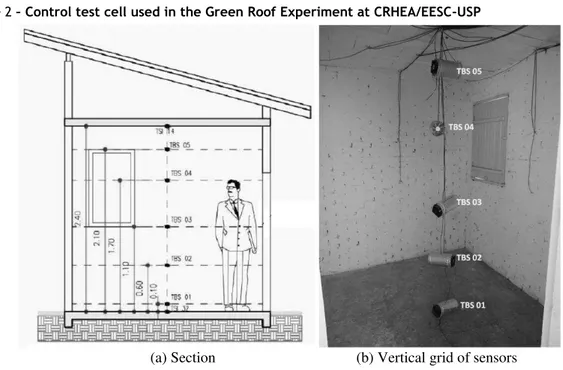
with a surface of about 1.3 m²; the ceiling height is 2.4 m. The roof consists of a tilted wooden structure covered with ceramic tiles and a ventilated crawl space above the wooden ceiling. Although not particularly large, the test cell resembles a typical building found in Brazilian social housing regarding building materials and openings (Figure 2).

Figure 1– Experimental site at CRHEA/EESC-USP

Figure 2– Control test cell used in the Green Roof Experiment at CRHEA/EESC-USP

(5)

Monitoring

Outdoor temperature data (dry bulb temperature) were monitored with a Campbell Scientific weather station using a CR10X logger. The indoor temperature data were measured with copper-constantan thermocouples at 30-minute intervals, sampled every hour. The accuracy was in the range 0.1-0.2°C (KINZIE, 1973). Although the indoor vertical temperature profile was monitored (with 5 dry bulb temperature sensors - TBS), we only used data registered at 1.10 m, at a height assumed to be representative of the mean indoor temperature conditions and which corresponds to the center of gravity of a standing person in the room (Figure 2). This height is considered to be adequate in human thermal comfort studies (LAMBERTS et al. 2016;

INTERNATIONAL…, 1998). Measurements were carried out without significant airflow in the room (door and window shut, as the proposed method is intended for environments with little or no ventilation).

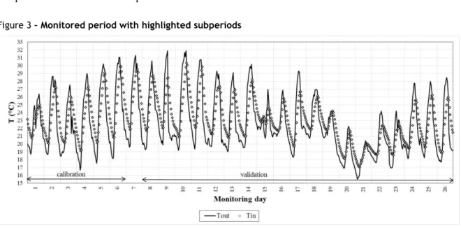
Twenty six days were monitored from 27 February, 2013 to 23 March, 2013. The first six days were used for the purpose of generating the change rate coefficient α; the seventh day was discarded as the necessary 24-h stabilization period for reaching a steady state; and the remaining 19 days were used for testing the model against the measured data (Figure 3).

Method proposed by Papst

This method is based on linear regression having as independent variable the running average of outdoor temperatures, which is statistically compared to the set of indoor temperature data to be

predicted, tentatively for increasing time steps. For the highest running average relationship to indoor temperatures, a linear model is generated. The method is applicable to buildings where indoor temperature fluctuations are low (PAPST, 2004). Thus, the first step is to determine the time frame needed for reaching the highest correlation between outdoor running averages versus indoor temperatures and the second step is to generate the predictive formula according to the following expression (Equation 1):

�� = ∑ �

−� −

�= ₊ _{Eq. 1}

Method proposed by the authors

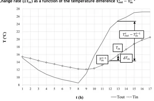
The predictive approach proposed in this paper describes hourly changes of the indoor temperature based on heat exchanges with the exterior and by using simple equations. The indoor air temperature changes at an hourly rate according to the inward or outward heat flow resulting from variations in outdoor meteorological conditions and from building envelope features. The heat balance normally sets in during nighttime in the absence of solar radiation. The proposed mathematical model estimates the rate of change of the indoor air temperature (∆�i ) as a function of the difference

between the outdoor temperature at a given hour (t) and the indoor temperature in the previous hour (t-1), � − �i−1 ), in a dynamic relationship

between such variables (Figure 4).

Mathematically, the predictive method can be expressed as follows (Equation 2):

�i = �i−1+ α � − �i−1 Eq. 2

(6)

Figure 4– Change rate (∆�_� ) as a function of the temperature difference � − �_�−�

The varying values found for change rate α expresses how the indoor environment reacts to outdoor temperature changes, in accordance with the definition of ‘thermal signature’ (GIVONI; VECCHIA; KRÜGER, 2002). The α coefficient is obtained using Equation 3 from measured data:

� = �� − ��−

� − �_�− Eq. 3

The change rate coefficient α will fluctuate throughout the day, assuming positive or negative values. However, it tends to stabilize around average values for a given trend, thus a simple mean value can be used for heat-gain conditions (e.g. according to a rising trend) and a different simple mean value for heat-loss conditions (as in a decreasing trend). A few days up to one week is a fairly sufficient period for calculating the change rate coefficients α.

For model validation, the first 24 hours should be discarded and are assumed as necessary for stabilizing predictions, since the first prediction takes the outdoor temperature measured at the previous hours as a trivial estimate for �i−1.

Three basic conditions are assumed for assessing the change rate coefficients α from the measured data:

(a) α = 0 is discarded, as this condition indicates an independent relationship of the variables involved, which does not conform to the dependency approach used in our model; (b) the modulus of α is used, which means that negative values are avoided. An advantage of using absolute values is that the scope of possible

models used for predicting this coefficient is amplified (in this case, exponential curves can also be used, although mean values, as used in this paper, can also yield satisfactory results); and (c) when temperature differences between outdoors and indoors (� − �� −1) are minimal,

i.e. when this factor comes close to zero, the change rate coefficient α can become increasingly unstable and exhibit very high values. Thus, a feasible interval must be determined for � −

�� −1, within which α-values are discarded. This

exclusion band can be assumed as -2 to +2 for high-mass test cells and -1 to +1 for low-mass test cells.

The flowchart shown in Figure 5 summarizes the predictive method proposed by the authors.

Results

In this section, the results are presented for both methods tested: the reference method used (PAPST, 2004) and the method proposed by the authors.

Reference model

The procedure described by Papst (2004) was adopted for the first six monitored days. Running averages of the outdoor temperatures were generated for the previous hour, two hours, three hours and so on, up to the 35th_{previous hour.} Pearson’s correlation coefficients were drawn between each running average and the dependent variable (�i ). The highest correlation was found for

the running average obtained from the previous seven hours (R = 0.986) (Figure 6).

� − �� −1

��

(7)

Figure 5– Flowchart of the predictive method

Figure 6– Correlation graph between the running average for the nth_{hour and the current indoor}

temperature

A linear relationship between the running average from the preceding 7th_{hour and the indoor} temperature was obtained by linear regression (Equation 4). This equation was used for the second monitoring period (19 days).

�� = . ∑ �

−� −

�= _{+ 5.} ₅ _{Eq. 4}

Proposed model

The same monitoring period was used for testing the method proposed in this paper. The period used for generating change rate coefficients α was 6 days; the 7th_{day was discarded (stabilization} period); and the validation period was 19 days, as described above.

APLICATION

Definition of time frame for calibration (from 4 to 7 days)

Calculation of mean alphas

Prediction of indoor temperatures

Discarding the first day of predicted data (steady state)

Assessing differences between estimated and measured data for the other days (bias analysis)

Accuracy check: differences are acceptable? (depending on the objectives of the study)

Yes No

Apply the method to other periods of interest

Try another method of prediction CALIBRATION

(8)

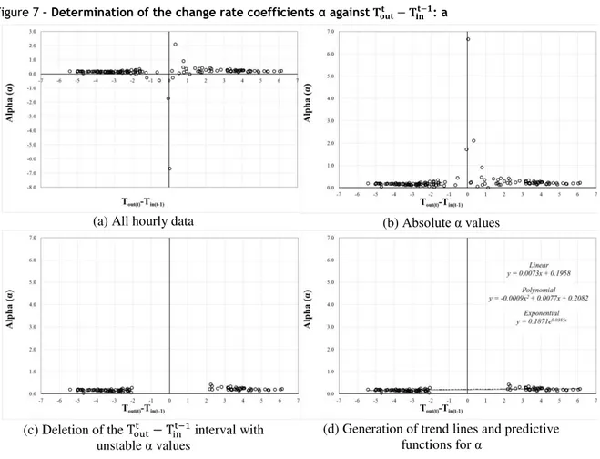
The mean change rate coefficient α was determined by identifying the rising rate and the decreasing rate (for warming and cooling trends, respectively) according to the three pre-conditions listed in the previous section. Figure 7 shows in a sequence: (a) scatter plots with all hourly data for α (negative and positive values);

(b) absolute values found;

(c) deletion of the interval with unstable conditions for α; and

(d) trend lines found for α.

The exclusion band for � − �i−1 was assumed as

-2 to +2 based on the scatter plot (Figure 7a). Mean values for the change rate coefficient α were obtained for a positive relationship of outdoor-indoor temperatures (rising rate) and for a negative relationship of � − �i−1 (decreasing rate),

yielding 0.23 and 0.17, respectively. The rate coefficient α for the positive relationship of outdoor-indoor temperatures tends to be higher than for a negative relationship, due to solar gains. Figure 8 shows the stabilization period needed for the model to reach a “steady state”. It can be noticed that a few hours would suffice to approximate predictions to actual temperature data.

Comparison of both models

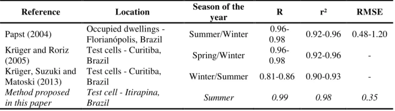
Table 1 shows a comparison between the measured and predicted data based on: Papst’s model and simple means for rising and decreasing rates (proposed model). The statistical analysis consists of the mean bias of estimate, mean absolute error, Root Mean Squared Error (RMSE), Pearson’s R, R -squared and Willmott’s index of agreement. The degree to which RMSE exceeds the mean absolute error ‘MAE’ is an indicator of the extent to which outliers (or variance in the differences between the modeled and observed values) exist in the data (LEGATES; MCCABE, 1999). Willmott’s measure varies from 0.0 to 1.0, with higher values indicating better agreement between the model and observations; this index overcomes the insensitivity of correlation-based measures to differences in the observed and model-simulated means and variances (LEGATES; MCCABE, 1999). It can be noticed that the model proposed shows better results, when compared to the method used by Papst. Even though Papst’s model has high correlations for measured data, the biases found are in a higher order of magnitude than in the model proposed in this paper. Figure 9 shows in a scatter plot differences found between measured and predicted indoor temperature data for both methods.

Figure 7– Determination of the change rate coefficients α against_{� − �}_�−�: a

(a) All hourly data (b) Absolute α values

(c) Deletion of the � − �i−1 interval with

unstable α values

(9)

Figure 8– Hourly data for measured vs. predicted indoor temperature concerning the measured outdoor temperature data – 24-h stabilization period

Table 1– Comparisons between measured and predicted indoor temperature data from different methods to assess the change rate coefficient α

Parameter Papst Simple means

mean bias of estimate (measured – predicted) (°C) -0.24 -0.02

maximum bias (°C) 1.40 1.06

mean absolute error (MAE) (°C) 0.52 0.28

RMSE 0.61 0.35

Pearson’s r 0.979 0.992

r-squared 0.959 0.983

Willmott’s index of agreement 0.986 0.996

Figure 9– Scatter plot with measured vs. predicted indoor temperatures for the second monitoring period

(10)

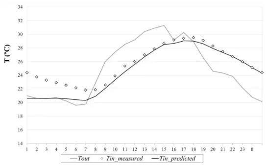
Figure 10 shows a comparison between measured and predicted indoor temperature data for the validation period and for the two prediction approaches.

It can be observed that even when there are sudden changes in the atmospheric conditions, no significant error is generated regarding the proposed method results. The model is more accurate regarding the daily minimum temperatures.

General discussion

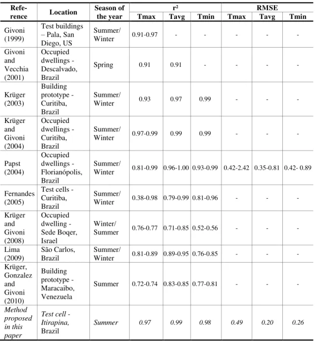
Results obtained from the predictive method presented in this paper can be compared to reported statistics from field studies cited in the Introduction and other selected studies worldwide concerning its predictive power. The approach used in all the field studies listed in Tables 2 and 3 is based on linear regression. Comparisons are drawn here in terms of hourly predictions (Table 2), as well as other studies with daily temperature predictions (Table 3); in the latter case daily averages were also calculated from hourly temperature predictions.

In general, the results obtained exhibit high predictive power in the case of hourly data, with good estimates for the daily average and minimum temperatures and a fairly good result in terms of RMSE for the daily maxima. The correlations found are in the order of magnitude of values reported in other field studies.

Conclusions

A predictive method was developed from experimental data based on temperature measurements in test cells, in which coefficients were estimated to describe the change rate of the indoor temperatures as a function of temperature differences between outdoors and indoors. Calibration and validation steps were conducted, as well as a comparison with other previous studies. The predictive method, although using a new approach, is a further development of existing black-box methods, as defined by Foucquier et al.

(2013) and most of them are based on a linear regression approach.

Figure 10– Hourly data for predicted indoor temperature plotted on the measured indoor temperature data - comparison between methods (Papst versus proposed method)

Table 2– Comparisons between reported studies and the proposed predictive method with hourly data

Reference Location Season of the

year R r² RMSE

Papst (2004) Occupied dwellings -_{Florianópolis, Brazil} Summer/Winter _0.980.96- 0.92-0.96 0.48-1.20 Krüger and Roriz

(2005)

Test cells - Curitiba,

Brazil Spring/Winter

0.96-0.98 0.92-0.96 -

Krüger, Suzuki and

Matoski (2013) Test cells - Curitiba, Brazil Winter/Summer 0.81-0.86 0.90-0.93 -

Method proposed in this paper

Test cell - Itirapina,

(11)

Table 3– Comparisons between reported studies and the proposed predictive method with derived daily data

Refe-rence Location

Season of the year

r² RMSE

Tmax Tavg Tmin Tmax Tavg Tmin

Givoni (1999)

Test buildings – Pala, San Diego, US

Summer/

Winter 0.91-0.97 - - - - -

Givoni and Vecchia (2001) Occupied dwellings -Descalvado, Brazil

Spring 0.91 0.91 - - - -

Krüger (2003) Building prototype - Curitiba, Brazil Summer/

Winter 0.93 0.97 0.99 - - -

Krüger and Givoni (2004) Occupied dwellings -Curitiba, Brazil Summer/

Winter 0.97-0.99 0.99 0.99 - - -

Papst (2004) Occupied dwellings -Florianópolis, Brazil Summer/

Winter 0.81-0.99 0.96-1.00 0.93-0.99 0.42-2.42 0.35-0.81 0.42- 0.89

Fernandes (2005)

Test cells - Curitiba, Brazil

Summer/

Winter 0.38-0.98 0.79-0.99 0.81-0.96 - - -

Krüger and Givoni (2008) Occupied dwelling - Sede Boqer, Israel Winter/

Summer 0.76-0.77 0.71-0.85 0.52-0.56 - - -

Lima (2009)

São Carlos, Brazil

Summer/

Winter 0.81-0.89 0.89-0.95 0.76-0.85 - - -

Krüger, Gonzalez and Givoni (2010) Building prototype - Maracaibo, Venezuela

Summer 0.72-0.74 0.83-0.85 0.77-0.81 - - -

Method proposed in this paper

Test cell - Itirapina,

Brazil

Summer 0.97 0.99 0.98 0.49 0.20 0.26

The method can be applied to research supported by test cells in cases where non-synchronous configurations (or experimental test runs) need to be compared as in typical normalized procedures. Advantages of the method presented could be in terms of:

(a) assessing the most promising operation modes of a given passive system; and

(b) allowing temperature predictions of a tested passive system for a different time period.

Considering the relevance of test-cell evaluations for testing building elements and/or operation modes of passive systems in terms of their low cost

the fact that they are easy to implement (when compared to prototype-supported evaluations), the simplicity of the predictive method further extends the scope of test-cell results by extrapolations of the background data. Note that we limit the application of the predictive method to naturally-ventilated or unconditioned buildings (i.e. passive systems), as the predictive approach is based on direct relationships between indoor and outdoor thermal environments.

(12)

driving factors behind the definition of the � − �i−1 band to be left out for obtaining mean α values

for rising/decreasing rates; and the effect of climatic variability between model generation and validation on prediction bias.

References

FERNANDES, L. C. Utilização de Equações Preditivas para Estimativa da Temperatura Interna de Edificações de Interesse Social. Curitiba, 2005. 187 f. Master (Thesis) – Programa de Pós-Graduação em Tecnologia, Universidade Tecnológica Federal do Paraná, Curitiba, 2005. FOUCQUIER, A. et al. State of the Art in

Building Modelling and Energy Performances Prediction: a review. Renewable and Sustainable Energy Reviews, v. 23, p. 272-288, 2013. GIVONI, B. Man, Climate and Architecture. [S.l.]: Barking, Applied Science Publishers, 1976. GIVONI, B. Minimum Climatic Information Needed to Predict Performance of Passive Buildings in Hot Climates. In: PASSIVE AND LOW ENERGY ARCHITECTURE

CONFERENCE, 16., Brisban, 1999. Proceedings... Brisban, 1999.

GIVONI, B.; GONZÁLEZ, E. Thermal

Performance of Indirect Evaporative Cooling in a Tropical Climate. In: NATIONAL SOLAR CONFERENCE, 38., Buffalo, 2009. Proceedings... Buffalo, 2009.

GIVONI, B.; KRÜGER, E. An Attempt to Base Prediction of Indoor Temperatures of Occupied Houses on Their Thermo-Physical Properties. In: PASSIVE AND LOW ENERGY

ARCHITECTURE, 20., Santiago do Chile, 2003. Proceedings... Santiago do Chile, 2003.

GIVONI, B.; VECCHIA, F. Predicting Thermal Performance of Occupied Houses. In: PASSIVE AND LOW ENERGY ARCHITECTURE, Florianópolis, 2001. Proceedings… Florianópolis, 2001.

GIVONI, B.; VECCHIA, F.; KRÜGER, E. Predicting Thermal Performance of Housing Types in Developing Countries with Minimum Climatic Data. In: WORLD CONGRESS OF

RENEWABLE ENERGY, 7., Cologne, 2002.

Proceedings… Cologne, 2002.

GONZALEZ, E.; KRÜGER, E. Evaluating the Potential of an Indirect Evaporative Passive Cooling System for Brazilian Dwellings. Building and Environment, v. 87, p. 265-273, 2015. HITCHIN, R. Editorial. Building and

Environment, v. 28, n. 2, p. 105–106, 1993.

HOFFMAN, M. E.; GIVONI, B. Prediction of Internal Temperature Using the Total Thermal time Constant as a Building Parameter,

Research Report, Building Research Station, Israel Institute of Technology, 1973.

INTERNATIONAL ORGANIZATION FOR STANDARDIZATION. ISO 7726: ergonomics of the thermal environment: instruments for

measuring physical quantities. Geneva, 1998. KINZIE, P. A. Thermocouple Temperature Measurement. New York: John Wiley & Sons, Inc., 1973.

KOMENO, M. H. Avaliação do Desempenho Térmico de Sistemas Construtivos Para

Habitações de Interesse Social Com a Utilização de Equações Preditivas e Simulação Por Meio de Software. Brasília, 2002. Undergraduate Final Project (Civil Engineering) – Universidade de Brasília, Brasília, 2002.

KOMENO, M. H.; KRÜGER, E.; SPOSTO, R. Avaliação do Desempenho Térmico de Sistemas Construtivos Para Habitação de Interesse Social Com a Utilização de Equações Preditivas. In: ENCONTRO NACIONAL SOBRE CONFORTO NO AMBIENTE CONSTRUÍDO, 7., Curitiba, 2003. Proceedings... Curitiba: ANTAC, 2003. KOTTEK, M. et al. World Map of the

Köppen-Geiger Climate Classification Updated.

Meteorologische Zeitschrift, v. 15, n. 3, 259-263, 2006.

KRÜGER, E. Aplicação de Equações Preditivas a Um Sistema Construtivo Destinado à Habitação de Interesse Social: avaliação de desempenho térmico em 11 cidades brasileiras. In: ENCONTRO NACIONAL SOBRE CONFORTO NO

AMBIENTE CONSTRUÍDO, 7., Curitiba, 2003. Proceedings... Curitiba: ANTAC, 2003.

KRÜGER, E.; DUMKE, E. Thermal Performance Evaluation of the Technological Village of Curitiba – Brazil. In: PASSIVE AND LOW ENERGY ARCHITECTURE, Florianópolis, 2011.

Proceedings… Florianópolis: PLEA, 2001.

KRÜGER, E.; FERNANDES, L. C. Error Analysis of Temperature Predictions for the Indoor

Temperature in Low-Cost Houses. In: PASSIVE AND LOW ENERGY ARCHITECTURE; CONFERENCE ON PASSIVE AND LOW ENERGY ARCHITECTURE -

ENVIRONMENTAL SUSTAINABILITY THE CHALLENGE OF AWARENESS IN

DEVELOPING SOCIETIES, 22., Beirut, 2005.

(13)

KRÜGER, E.; GIVONI, B. Predicting Thermal Performance in Occupied Dwellings. Energy and Buildings, v. 36, n. 3, p. 301-307, 2004.

KRÜGER, E.; GIVONI, B. Thermal Monitoring and Indoor Temperature Predictions in a Passive Solar Building in an Arid Environment. Building and Environment, v. 43, n. 11, p. 1792-1804, 2008.

KRÜGER, E.; GONZALEZ, E.; GIVONI, B. Effectiveness of Indirect Evaporative Cooling and Thermal Mass in a Hot Arid Climate. Building and Environment, v. 45, n. 6, p. 1422-1433, 2010.

KRÜGER, E.; PAPST, A L. Aferição de Equações Preditivas da Temperatura Ambiente Quando Aplicadas a Uma Série de Dados Mais Recente. In: ENCONTRO NACIONAL SOBRE CONFORTO NO AMBIENTE CONSTRUÍDO, 7., Curitiba, 2003. Proceedings... Curitiba: ANTAC, 2003. KRÜGER, E.; RORIZ, M. Previsão Horária de Temperaturas Internas do Ar: aplicação no estudo de células teste. In: ENCONTRO NACIONAL SOBRE CONFORTO NO AMBIENTE

CONSTRUÍDO, 8., Maceió, 2005. Proceedings…

Maceió: ANTAC, 2005.

KRÜGER, E.; SUZUKI, E.; MATOSKI, A. Evaluation of a Trombe Wall System in a Subtropical Location. Energy and Buildings, v. 66, p. 364-372, 2013.

LAMBERTS, R. et al. A Nova Proposta de Norma

Brasileira de Conforto Térmico. Conforto e Stress Térmico, Florianópolis, 2016.

LEGATES, D. R.; MCCABE, G. J. Evaluating the Use of “Goodness-of-fit” Measures in Hydrologic and Hydroclimatic Model Validation. Water Resources Research, v. 35, n. 1, p. 233-241, 1999.

LIMA, M. P. Equações Preditivas Para Determinar a Temperatura Interna do Ar: envolventes em painel alveolar com cobertura verde. São Carlos, 2009. Master Thesis (Programa de Pós-Graduação em Engenharia Ambiental) – Universidade de São Carlos, São Carlos, 2009. MARQUES, A. M. Desempenho Térmico de Edificações Unifamiliares de Interesse Social: estudo de casos em Imbituba. Florianópolis, 2008. Master Thesis (Programa de PósGraduação em Engenharia Civil) – Universidade Federal de Santa Catarina, Florianópolis, 2008.

PAPST, A. L. Método Estimativo da Temperatura Interna de Edificações

Residenciais em Uso. PhD Thesis (Programa de Pós-Graduação em Engenharia Civil) –

Universidade Federal de Santa Catarina, Florianópolis, 2004.

PAPST, A. L.; LAMBERTS, R. Relacionamento da Temperatura Interna e Externa em Edificações Residenciais Naturalmente Ventiladas. In: ENCONTRO NACIONAL SOBRE CONFORTO NO AMBIENTE CONSTRUÍDO, 6., São Pedro, 2001. Proceedings... São Pedro: ANTAC, 2001. SEIXAS, G. T. Climatologia Aplicada à Arquitetura: investigação experimental sobre a distribuição de temperaturas internas em duas células de teste. 2005. PhD Thesis (Programa de Pós-Graduação em Construção Civil) –

Universidade Federal de São Carlos, São Paulo, 2015.

STRACHAN, P. A.; BAKER, P. H. Outdoor Testing, Analysis and Modelling of Building Components. Building and Environment, v. 43, n. 2, p. 127–128, 2008.

(14)

Eduardo Leite Krüger

Leandro Fernandes

Grace Tibério Cardoso

Emilio Eiji Kavamura

Departamento de Expressão Gráfica | Universidade Federal do Paraná | E-mail: emilio.kavamura@ufpr.br

Revista Ambiente Construído

Associação Nacional de Tecnologia do Ambiente Construído Av. Osvaldo Aranha, 99 - 3º andar, Centro

Porto Alegre – RS - Brasil CEP 90035-190 Telefone: +55 (51) 3308-4084

Fax: +55 (51) 3308-4054 www.seer.ufrgs.br/ambienteconstruido