automata models with socioeconomic
heterogeneity
Interpretação do uso do solo para modelos de autômatos
celulares com heterogeneidade socioeconômica
Bernardo Alves Furtado
Abstract
ellular automata models for simulation of urban development usually lack the social heterogeneity that is typical of urban environments. In order to handle this shortcoming, this paper proposes the use of supervised clustering analysis to provide socioeconomic intra-urban land use classification at different levels to be applied to cellular automata models. An empirical test in a highly diverse context in the Greater Metropolitan Area of Belo Horizonte (RMBH) in Brazil is provided. The results show that a reliable division into different socioeconomic land-use classes at large scale enable detailed urban dynamic analysis. Furthermore, the results also allow the quantification of the proportion of urban space occupation for different levels of income; (2) and their pattern in relation to the city centre.
Palavras-chave: Cellular automata models. Urban development. RMBH. Supervised clustering analysis.
Resumo
Modelos de autômatos celulares para simulação da dinâmica urbana usualmente não incluem heterogeneidades sociais, típicas do espaço urbano. No intuito de lidar com tais falhas, este texto propõe a utilização de análise de agrupamento supervisionada para prover classificação em diferentes níveis socioeconômicos do uso do solo intra-urbano para utilização em modelos de autômatos celulares. Um teste empírico é aplicado no contexto altamente diversificado da Região
Metropolitana de Belo Horizonte (RMBH). Os resultados demonstram que divisão de classes socioeconômicas de uso do solo em grande escala permite análise da dinâmica urbana detalhada. Além disso, os resultados permitem a quantificação da proporção da ocupação espacial urbana para os diferentes níveis de renda; e seu padrão em relação à localização do centro urbano.
Keywords: Modelos de autômatos celulares. Desenvolvimento urbano. RMBH. Aanálise de agrupamento supervisionada.
C
Bernardo Alves Furtado
Diretoria de Estudos Regionais e Urbanos. Instituto de Pesquisa Econômica Aplicada SBS, Quadra 1, Bloco J, Ed. BNDES Brasilia - DF - Brasil CEP 70076-900 Tel.: (61) 3315-5194 E-mail: [email protected]
Introduction and literature
A number of cellular automata (CA) models have been used to shed light on the complex processes of urban development. The early works of JohnConway‟s „Game of Life‟ (BERLEKAMP, 2004; GARDNER, 1970), and Thomas Schelling seminal paper on segregation (1978) initiated a proficuous production of CA models in economics (ARTHUR, 1994; HOLLAND, 1992), urban morphology (ALLEN, 1997; BATTY, 1998; WHITE; ENGELEN, 1993), and social science (PORTUGALI, 2000). These early ideas unfolded onto a full series of simulation models specifically designed for urban environment. They are comprehensively reviewed by Benenson and Torrens (2004), and Batty (2005a). One example of such simulation models is UrbanSim (WADDELL; ULFARSSON, 2003; WADDELL
et al., 2007). UrbanSim investigates the influence
of transport on land use and its feedbacks, at a large scale, and in an environment of modules that includes macroeconomics analysis, housing property prices, and housing development. Another example is the pioneering work of Keith Clarke et al. (1997) which was further developed
into the SLEUTH model (SILVA; etCLARKE, 2002) – an acronym for Slope, Land, Excluded areas, Urban extent, Transportation and Hillshade.
The emphasis of SLEUTH is on the „brutal force‟
method which is applied to find the best parameters for a given situation. These parameters in turn provide the best forecasting. Other models include Object-Based Environment for Urban Simulation (OBEUS) developed by Benenson et al. (2006), and Environment Explorer (ENGELEN et al., 2005) developed at Research Institute for
Knowledge Systems (RIKS). This intense use of CA models reinforced the quest for theoretical fundamentation (HAGOORT, 2006), as well as discussions on comparability of methods and models (PONTIUS et al., 2008), validation
procedures (BROWN, 2005), and metrics on quantification of changes and comparisons (HAGEN-ZANKER, 2005).
These developments are based on data of land use captured by remote sensing imagery, and processes, such as land classification. Therefore, most applications rely on categories of land use that distinguish urban areas (also referred to as residential areas), from forestry, industry, agriculture, water bodies, and sometimes commerce. According to Pontius and colleagues (2008), the choice of land use classes may vary from two (urban, and non-urban; Geomod, in Worcester, USA) up to 15 (Environment Explorer, The Netherlands). Nevertheless, none of these models observe an intra-urban division of land use
classes that accounts for urban diversity. That is, it is rare to see a division of urban land use classes that accounts for the rich division of urban uses
that actually happen within cities‟ realms.
Given the understanding of the city as a socioeconomic complex phenomena (SOJA, 2000), we argue that a model aiming at simulating urban development cannot fail to address cities‟
internal social heterogeneities. This view coincides with Fernandez‟s et al. (2005) concluding
recommendations for agent-based models. He says
that when “simulating resident behaviour, [the model] should reflect this diversity in the population and incorporate distinct agent classes of
empirically derived preference distributions”
(FERNANDEZ et al., 2005, p. 818).
In fact, the use of one single class that defines residential areas opposed to all others is neither compatible with the stylized fact that cities are spatially segregated, nor are they with the georeferenced data largely available. Both Hubacek and Bergh (2006) and Meng et al. (2006)
agree that land use analysis should be viewed explicitly spatially, use full detailed data (rather than sampled aggregated information), and include multidisciplinary views. Aggregated data implicitly produces analyses that are too general to
fully incorporate cities‟ idiosyncrasies. If the aim
is to study diversities across the city, Hardman anf Ionnides (2003) strongly recommends that the analysis should be made at a large scale, considering only the closest neighbors – which are more likely to have homogeneous attributes. This vision is corroborated by Meng et al. (2006, p.
278) who argues that local measures are helpful in
identifying “spatial pockets of distinct segregated values”.
In order to handle the shortcoming in availability of socioeconomically divided land categories, we propose the use of supervised clustering analysis –
which is usually applied in remote sensing and physical geography. However, instead of applying it to image acquired through remote sensing, we apply it to the census tract income questionnaires‟
answers. Further, we apply some metrics on quantifying maps originally developed in ecological studies to help pinpoint spatial configurations of the different land classes proposed, and its dynamics.
inhabitants can be described precisely in space and time. Thus, it reinforces analysis that is usually done on qualitative terms and is very dependent on
the researchers‟ knowledge of the area. Secondly,
it provides a snapshot of land occupation of physical space in the city by level of income. Thirdly, the spatialization of level-income categories in the city allows the empirical check of the long-lasting assumption of land-use classes positioning in relation to the Centre Business District (CBD). Thünen (em 1826) (THÜNEN, 1966) established that for agricultural land use, in a homogeneous prairie, in equilibrium, the crop that yields the higher value per area would locate closest to the market. William Alonso (1964) adapted and transferred these ideas into urban context, but maintained the logic that business and firms would be able to pay the premium price to locate at the centre. These seminal works are at the core of Urban Economics. Despite having advanced much since then (CAPELLO; NIJKAMP, 2004), this field of science retains
„distance to CBD‟ as a core factor (LUCAS; ROSSI-HANSBERG, 2002). The classification of residential land use by income enables the empirical checking of this reality. From the results it is easy to see that these assumptions hold in general, when observing the city as a whole. When the level of the analysis is the large scale, however, it is clear that there is no simple pattern of presence of land uses in relation to the city centre. All in all, the exercise provided in this paper shows that intra-urban analysis has much to gain qualitatively if it makes full use of quantitative information broadly available. In fact, the contribution of this paper in terms of science knowledge aggregation is manifold. Broadly speaking, it contributes to the cross-fertilization of science fields when using typical remote sensing technology applied to socioeconomic analysis, usually studied in an a-spatial framework. Further, the paper also demonstrates that urban economics general assumptions can be put to test given contemporaneous availability of data and technology. Finally, the text also makes it clear that analysts and local public workers are enabled to pinpoint change as well as configuration of socioeconomic information to a precise level within their municipality. Together these contributions are within the scope of technologies of the constructed environment as they depict method and data techniques which empower scientists and managers alike to a higher level of knowledge at intraurban level and therefore enable them to propose and act upon policies in the areas of housing, sanitation and urban mobility. Most of all, hints on the processes of cities evolution based
on socioeconomic characteristics foster dynamic analysis which may contribute to the design, review and amelioration of urban public policies. The empirical exercise is applied to the conurbated municipalities of the Greater Area of Belo Horizonte (RMBH), in Brazil, with data from two census years: 1991 and 2000. At least two moments in time are necessary to evaluate performance of cellular automata models of urban development (PONTIUS et al., 2008).
The remainder of the study presents the methodology and data used, discusses the metrics applied, the results and some conclusions.
Methodology: multivariate
analysis
–
clustering
If one thinks of comprehensive socioeconomic data in terms of household characteristics the immediate source of information is census data. Census data are usually available by census tracts1
only, so that specific personal family information is kept secret. Further, census tract are usually the most detailed spatial information available. When it comes to spatial analysis researchers are usually interested in relations of proximity, distance, and relative location across each piece of data.
The methodology put forward in this section aims at making household characteristics and its location useful for spatial analysis. We do so in three steps. Firstly, by counting domiciles in each census tract which belong to each pre-available class of income. Secondly, by using those layers of information to create maps where the data is spatially distributed. Ant thirdly, aggregating the data spatially in order to provide analytical input for urban studies. The first step is statistical, the second is a transformation – from vector data by census tract into raster matrix data; and the third is an aggregative methodology as detailed in the next paragraphs.
The method of clustering might be characterized as any statistical proceeding that from a finite and multidimensional set of data classifies its elements in restricted, internally homogeneous groups which enable the constructions of aggregated structures and typologies (Simões, 2003; 2005). Clustering has been used in real estate by Bourassa
et al. (1999), and in agent-based modeling by
Fernandez et al. (2005) among others, and it has
been used extensively in ecological studies and natural sciences (LILLESAND et al., 2004).
In the proposed clusterization “train samples” are
used, i.e., samples of locations in which the researcher is sure that they belong to a certain class he or she is trying to make the typologies of. Samples are, therefore, those regions of the city in which we are absolutely sure that they belong to one of the specific intended classes. In a second
moment, the classes‟ configuration is determined
in a maximum likelihood classification which assigns (through distance calculation) all cells of the study as belonging to the most likely class. When the sample provides a large enough number of cells, the classification presents higher guarantees.
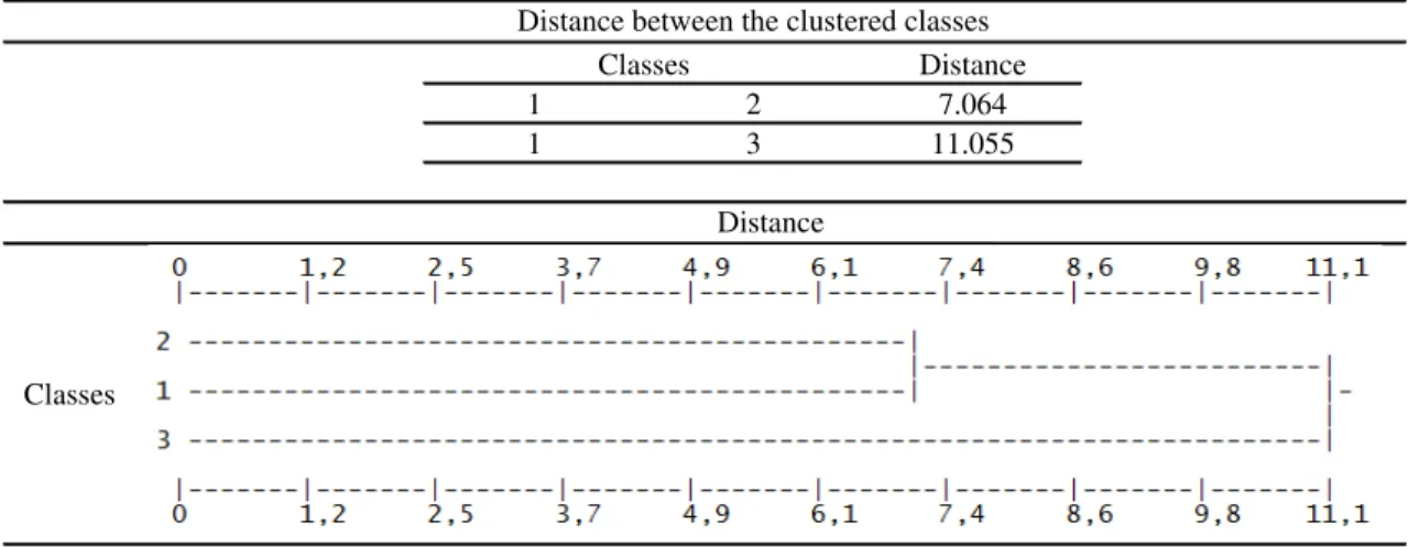
Two are the main results of the procedures of the clustering technique:
(a) the dendogram which shows visually the distance between the classes elaborated, and enables the verification of how close or how distant it is from the other classe2; and
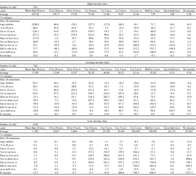
(b) the average and co-variance of the cells of each typical class which enable the understanding, and confirmation of the characteristics of each class.
In this study, we propose the clusterization into three classes representing income levels which are thought to capture implicit social heterogeneity. Therefore, the classes chosen are the following levels:
(a) high-income; (b) average-income; and (c) and low-income.
Metrics on quantifying maps
In order to have additional parameters to compare and validate the results with cellular automata models, despite the visual description (CLARKE
et al., 1997), some metrics typically used in
ecological studies and physical geography (MCGARIGAL et al., 2002; VISSER; NIJS, 2006)
are presented. They are also referred to by Brown and colleagues (2005).
Most of the metrics are based on „patch size‟ which is defined as “[…] groups of contiguous cells that are taken in by the same category […]”
(HAGEN-ZANKER, 2006, p. 171). Given the
2“The dendogram tool uses a hierarchical clustering algorithm.
The program first computes the distances between each pair of classes in the input signature file. Then, it iteratively merges the closest pair of classes and successively merges the next closest pair of classes and the succeeding closest until the classes are all merged. After each merging, the distances between all pairs of classes are updated. The distances at which the signatures of classes are merged are used to construct a dendogram [...]” (ESRI, 2006).
patch definition, one can measure its size, perimeter and edge length. Other common (and popular) descriptive numbers are fractal dimension and the shape index (BATTY, 2005b; BATTY; LONGLEY, 1994; BENENSON; TORRENS, 2004). Fractal dimensions provide a single number for a map which indicates how much space is completely filled with a certain state or category. Among some other specifications (BATTY, 2005b), it might be given as Eq. 1 (MCGARIGAL
et al., 2002):
ij ij
lna 0.25p 2ln
F Eq. 1
Where,
F is the fractal dimension; pij is the perimeter of each patch;
ij and aij is the area of patch ij.
The intuition behind it is that the fractal dimension represents the complexity of the shape. A number close to 2, for instance, would represent a square nearly filled with the same state. The shape index, in turn, is calculated as the perimeter divided by the square root of the patch size. It is easy to see
that “larger values indicate a more convoluted shape” (RIKS, 2006, p. 33).
A number of computer programs to calculate these measures is available, such as The Map Comparison Kit, developed within RIKS B.V.; and Fragstats, developed by the University of Massachusetts (MCGARIGAL et al., 2002).
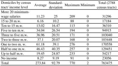
Table 1 – Basic statistics of domiciles by census tract and levels of income, year 1991
Domiciles by census
tract/ income level Average
Standard-deviation Maximum Minimum
Total (2788 census tracts) More 20
minimum-wage salaries 11.23 25 209 0 31296
15 to 20 m.w. 6.16 10.2 88 0 17184
Ten to 15 m.w. 13.02 16.47 113 0 36310
Five to ten m.w. 34.04 26.54 194 0 94915
Three to five m.w. 36.96 20.51 171 0 103040
Two to three m.w. 37.1 20.07 168 0 103448
One to two m. w. 61.18 39.1 276 0 170558
Half to one m.w. 46.43 40.35 257 0 129451
Up to half m.w. 19.45 24.87 233 0 54217
No income 8.27 9.19 91 0 23056
Total 273.84 92.79 770 2 763475
Table 2 – Basic statistics of domiciles by census tract and levels of income, year 2000 Domiciles by census
tract/ income level Average
Standard-deviation Maximum Minimum
Total (4121 census tracts) More 20
minimum-wage salaries 14.49 31.35 323 0 59707
15 to 20 m.w. 9.1 12.78 75 0 37502
Ten to 15 m.w. 12.57 13.15 80 0 51819
Five to ten m.w. 41.19 26.96 252 0 169736
Three to five m.w. 39.75 20.71 201 0 163801
Two to three m.w. 31.8 18.57 203 0 131947
One to two m. w. 47.67 32.41 396 0 196465
Half to one m.w. 31.81 22.76 206 0 131081
Up to half m.w. 1.23 1.84 16 0 5055
No income 21.71 19.87 290 0 89466
Total 251.32 80.41 1306 11 1035679
Data
The data used in this study is composed of the polygons that determine census tract limits for the year 2000 (INSTITUTO…, 2003) elaborated and defined by Brazilian Statistics Foundation (IBGE); along with the number of domiciles per classes of income 3 for both census years of 1991
(INSTITUTO…, 1991; 2003). As part of Brazilian statistical procedures, every 10 years data is collected from all possible households of the country. In this section the data is available by census tract. Each tract contains the number of household in each pre-established income classes as defined by the institute responsible for the
3 The classes of income available are families whose income are:
(1) above 20 minimum-wage salaries; (2) from 15 to 20 minimum-wage salaries; (3) from ten to 15 minimum-wage salaries; (4) from five to ten minimum-wage salaries; (5) from three to five minimum-wage salaries; (6) from two to three minimum-wage salaries ; (7) from one to two minimum-wage salaries; (8) from half minimum-wage salary to one; (9) up to half minimum-wage salary; and (10) no income.
census (IBGE). Some general statistics of the data are presented in Table 1 and Table 2.
In order to enable the supervised clustering procedure, the data available in vector format (table data associated with the polygons) is transformed into raster map (a grid format in which every cell – in this case of 86 by 86 meters –
receives the value in the table). This is a straightforward procedure available for any Geographical Information System (GIS) software4.
The area of the study comprises the capital of Minas Gerais state, Belo Horizonte, and the neighboring municipalities, which together configure the conurbated urban area of the Greater Area of Belo Horizonte5, and holds 90% of its
population.
4 For this case ARCMap, from ESRI, was used.
5 The referred municipalities are, namely: (1) Betim, (2)
Distance
1 2 7.064
1 3 11.055
Distance between the clustered classes Classes
Distance
Classes
Figure 1 - Dendogram of clusterization year 1991
Distance
1 2 8.169
1 3 18.499
Distance Classes
Distance between the clustered classes
Classes
Figure 2 - Dendogram of clusterization year 2000
Methodological note on the data
availability for year 1991
Information for the year 1991 is only available in table format, not spatially. That means that the polygons that describe each census tract are unavailable. What the government foundation (IBGE) did provide were two tables of correlation so that census tract codes of 2000 – for which there are the polygons – were associated to the census
tract codes of 1996‟s population count and codes
of 1996 were linked to those of 1991.
In constructing the 1991‟s map database, the codes
were related to each other within a Microsoft Access database framework. The polygon map of
1991‟s 2,788 census tracts is then the result of the aggregation of 2000‟s 4,121 ones.
Some inconsistencies are noted because not all 2000 census tracts are disaggregation of those
existent in 1991. Actually, IBGE‟s construction of
census tracts is reviewed at every census occasion and given its need of a certain homogeneity and average size, a new tract might be an addition of
parts of two old ones. Therefore, given the procedures used to produce the map, for some observations the values of income information were different for the same tract; e.g. in the case that a tract in 2000 had a part belonging to a tract in 1991 and part belonging to another one. As a rule, every time this occurred, the maximum value was chosen. Visual inspection on the results were performed along with general comparison with results provided by Mendonça (2002). The comparisons confirmed that these inconsistencies were minor ones, and that they did not affect the overall ability of the map to represent land uses in 1991. Whereas the results do not have a 100% confidence, they provide the best analysis of income spatially distributed at this scale that we know of.
Train samples for supervised
clusterization
In the proposed case the „train samples‟ have as
neighborhoods‟ classification scheme performed
by a research institute affiliated with the Federal University of Minas Gerais (UFMG), called Foundation Institute of Economic, Administrative and Accountancy Research of Minas Gerais (IPEAD)6.
Results and discussion
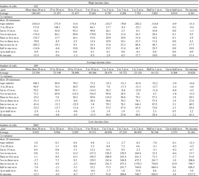
Results of the clustering procedures
The clustering made for the RMBH presents well-defined classes for both years 1991 and 2000 (Figure 1 and Figure 2). That is, the distance between the classes is large enough so that adifferent typology is clearly established. Note, however that the distance is much larger for the year 2000. The important aspect of the supervised clusterization is that the resulting clusters yield clearly divided typologies which are comparable. The analysis of Tables 3 and 4 indicate – by their more expressive number of cells – that high-income class concentrates domiciles in which the household has income above 20 minimum-wage salaries. The average-income class has its highest value in the interval between 5 and 10 minimum-wage salaries and the low-income class is comprised mostly of households whose income is of one minimum-wage salary.
Table 3 - Average and co-variance for supervised clusterization year 1991
Number of cells 514
Layer More than 20 m.w. 15 to 20 m.w. 10 to 15 m.w. 5 a 10 m.w. 3 a 5 m.w. 2 a 3 m.w. 1 to 2 m. w. Half to 1 m.w. Up to half m.w. No income
Average 107.02 29.17 37.56 37.40 13.08 9.07 12.46 7.59 3.60 2.98
Co-variance More 20
minimum-wage salaries 1208.8 80.8 -129.1 -257.2 -127.9 -80.9 19.1 71.7 16.6 16.5
15 to 20 m.w. 80.8 99.2 63.9 54.3 1.9 -18.2 -59.9 -48.3 -21.7 8.5
Ten to 15 m.w. -129.1 63.9 187.0 159.5 39.3 2.7 -74.1 -80.0 -31.0 0.8
Five to ten m.w. -257.2 54.3 159.5 323.6 90.8 38.5 -45.2 -60.6 -16.8 3.8
Three to five m.w. -127.9 1.9 39.3 90.8 55.8 35.6 47.0 33.5 17.5 0.6
Two to three m.w. -80.9 -18.2 2.7 38.5 35.6 50.0 103.5 94.4 42.2 1.4
One to two m. w. 19.1 -59.9 -74.1 -45.2 47.0 103.5 346.0 333.2 142.6 2.7
Half to one m.w. 71.7 -48.3 -80.0 -60.6 33.5 94.4 333.2 351.7 148.9 -0.1
Up to half m.w. 16.6 -21.7 -31.0 -16.8 17.5 42.2 142.6 148.9 64.3 -0.2
No income 16.5 8.5 0.8 3.8 0.6 1.4 2.7 -0.1 -0.2 5.6
Number of cells 744
Layer More than 20 m.w. 15 to 20 m.w. 10 to 15 m.w. 5 to 10 m.w. 3 to 5 m.w. 2 to 3 m.w. 1 to 2 m.w. Half to 1 m.w. Up to half m.w. No income
Average 17.09 13.60 31.97 70.29 46.06 30.57 32.14 19.28 8.15 5.54
Co-variance More 20
minimum-wage salaries 95.3 40.1 75.2 63.8 -21.1 -39.3 -59.0 -51.5 -29.0 -3.6
15 to 20 m.w. 40.1 45.6 68.8 87.5 16.1 -7.2 -25.8 -24.4 -10.0 -0.2
Ten to 15 m.w. 75.2 68.8 182.4 221.4 63.1 12.6 -45.5 -33.9 -27.6 0.5
Five to ten m.w. 63.8 87.5 221.4 538.7 216.4 107.4 20.8 13.3 -8.4 9.5
Three to five m.w. -21.1 16.1 63.1 216.4 202.3 109.1 87.8 74.3 38.4 15.0
Two to three m.w. -39.3 -7.2 12.6 107.4 109.1 110.1 87.2 69.4 40.3 7.1
One to two m. w. -59.0 -25.8 -45.5 20.8 87.8 87.2 150.8 102.4 53.2 10.7
Half to one m.w. -51.5 -24.4 -33.9 13.3 74.3 69.4 102.4 129.5 56.6 8.9
Up to half m.w. -29.0 -10.0 -27.6 -8.4 38.4 40.3 53.2 56.6 104.7 3.0
No income -3.6 -0.2 0.5 9.5 15.0 7.1 10.7 8.9 3.0 17.7
Number of cells 1428
Layer More than 20 m.w. 15 to 20 m.w. 10 to 15 m.w. 5 to 10 m.w. 3 to 5 m.w. 2 to 3 m.w. 1 to 2 m.w. Half to 1 m.w. Up to half m.w. No income
Average 1.392 0.647 2.660 11.543 25.392 35.445 106.892 130.961 62.131 19.567
Co-variance More 20
minimum-wage salaries 1.0 0.1 0.4 0.8 1.1 -2.7 -8.2 -7.6 -0.1 -12.3
15 to 20 m.w. 0.1 1.1 0.8 5.2 8.8 7.2 4.8 -2.1 -0.3 -4.5
Ten to 15 m.w. 0.4 0.8 3.3 12.2 14.1 9.5 -2.3 -5.1 -0.2 -6.7
Five to ten m.w. 0.8 5.2 12.2 127.2 156.5 129.5 104.4 33.2 -0.4 13.7
Three to five m.w. 1.1 8.8 14.1 156.5 288.9 243.4 241.3 73.3 -1.7 51.0
Two to three m.w. -2.7 7.2 9.5 129.5 243.4 349.8 475.2 241.7 1.0 208.6
One to two m. w. -8.2 4.8 -2.3 104.4 241.3 475.2 1176.3 744.0 15.9 748.7
Half to one m.w. -7.6 -2.1 -5.1 33.2 73.3 241.7 744.0 684.4 8.6 656.5
Up to half m.w. -0.1 -0.3 -0.2 -0.4 -1.7 1.0 15.9 8.6 4.2 3.0
No income -12.3 -4.5 -6.7 13.7 51.0 208.6 748.7 656.5 3.0 1317.2
High-income class
Low-income class Average-income class
6
6 In the present study the following neighbourhoods areas serve as reference for high-income classes: Lourdes, Sion, Mangabeiras,
Table 4 - Average and co-variance for supervised clusterization year 2000
Number of cells 422
Layer More than 20 m.w. 15 to 20 m.w. 10 to 15 m.w. 5 to 10 m.w. 3 to 5 m.w. 2 to 3 m.w. 1 to 2 m.w. Half to 1 m.w. Up to half m.w. No income
Average 148.443 31.457 21.457 22.661 6.787 4.268 7.763 3.865 0.014 4.261
Co-variance More 20
minimum-wage salaries 2414.4 171.0 14.4 -174.4 -132.7 -70.0 -202.2 -114.6 -0.9 -31.4
15 to 20 m.w. 171.0 148.1 92.0 84.1 13.7 -8.5 -25.1 -6.6 -0.1 -9.4
Ten to 15 m.w. 14.4 92.0 95.2 99.0 26.1 2.5 8.3 10.8 0.0 -1.3
Five to ten m.w. -174.4 84.1 99.0 179.0 53.8 12.4 24.3 20.4 0.1 0.5
Three to five m.w. -132.7 13.7 26.1 53.8 29.9 10.9 31.6 19.2 0.1 2.9
Two to three m.w. -70.0 -8.5 2.5 12.4 10.9 10.1 23.3 13.4 0.0 6.5
One to two m. w. -202.2 -25.1 8.3 24.3 31.6 23.3 86.4 48.7 -0.1 17.7
Half to one m.w. -114.6 -6.6 10.8 20.4 19.2 13.4 48.7 29.3 0.0 10.0
Up to half m.w. -0.9 -0.1 0.0 0.1 0.1 0.0 -0.1 0.0 0.0 0.0
No income -31.4 -9.4 -1.3 0.5 2.9 6.5 17.7 10.0 0.0 11.4
Number of cells 489
Layer More than 20 m.w. 15 to 20 m.w. 10 to 15 m.w. 5 to 10 m.w. 3 to 5 m.w. 2 to 3 m.w. 1 to 2 m.w. Half to 1 m.w. Up to half m.w. No income
Average 25.550 23.198 28.898 69.266 38.479 19.722 23.110 16.121 0.368 10.826
Co-variance More 20
minimum-wage salaries 198.3 94.9 70.2 73.2 -25.2 -51.3 -81.6 -52.2 -2.9 -14.6
15 to 20 m.w. 94.9 74.3 50.5 65.0 7.0 -17.3 -31.3 -13.7 -1.4 -4.8
Ten to 15 m.w. 70.2 50.5 91.1 114.3 28.2 -8.6 -22.9 -11.6 -0.6 -4.5
Five to ten m.w. 73.2 65.0 114.3 316.5 95.0 28.5 3.8 4.7 -1.8 -13.5
Three to five m.w. -25.2 7.0 28.2 95.0 119.2 58.6 79.3 57.2 1.9 29.5
Two to three m.w. -51.3 -17.3 -8.6 28.5 58.6 70.3 78.1 57.4 1.9 27.0
One to two m. w. -81.6 -31.3 -22.9 3.8 79.3 78.1 146.1 87.9 3.1 40.5
Half to one m.w. -52.2 -13.7 -11.6 4.7 57.2 57.4 87.9 72.0 2.3 29.4
Up to half m.w. -2.9 -1.4 -0.6 -1.8 1.9 1.9 3.1 2.3 0.5 2.2
No income -14.6 -4.8 -4.5 -13.5 29.5 27.0 40.5 29.4 2.2 43.3
Number of cells 2065
Layer More than 20 m.w. 15 to 20 m.w. 10 to 15 m.w. 5 to 10 m.w. 3 to 5 m.w. 2 to 3 m.w. 1 to 2 m.w. Half to 1 m.w. Up to half m.w. No income
Average 0.925 0.904 2.029 19.311 40.856 47.210 86.892 56.346 2.553 51.461
Co-variance More 20
minimum-wage salaries 1.0 0.1 0.4 0.8 1.1 -2.7 -8.2 -7.6 -0.1 -12.3
15 to 20 m.w. 0.1 1.1 0.8 5.2 8.8 7.2 4.8 -2.1 -0.3 -4.5
Ten to 15 m.w. 0.4 0.8 3.3 12.2 14.1 9.5 -2.3 -5.1 -0.2 -6.7
Five to ten m.w. 0.8 5.2 12.2 127.2 156.5 129.5 104.4 33.2 -0.4 13.7
Three to five m.w. 1.1 8.8 14.1 156.5 288.9 243.4 241.3 73.3 -1.7 51.0
Two to three m.w. -2.7 7.2 9.5 129.5 243.4 349.8 475.2 241.7 1.0 208.6
One to two m. w. -8.2 4.8 -2.3 104.4 241.3 475.2 1176.3 744.0 15.9 748.7
Half to one m.w. -7.6 -2.1 -5.1 33.2 73.3 241.7 744.0 684.4 8.6 656.5
Up to half m.w. -0.1 -0.3 -0.2 -0.4 -1.7 1.0 15.9 8.6 4.2 3.0
No income -12.3 -4.5 -6.7 13.7 51.0 208.6 748.7 656.5 3.0 1317.2
High-income class
Low-income class Average-income class
Analysis: year 1991
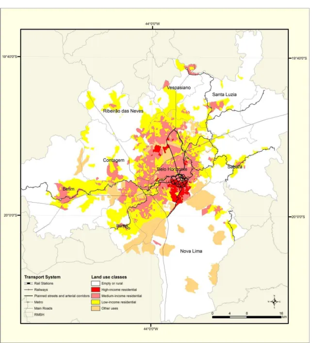
This section describes in detail the spatial configuration of RMBH in the year 1991. The analysis of Figure 3 shows that the high-income residential area is clustered southern of the original planned area7 with some other locations further
north. The morphology is convoluted – although concentrated –, and areas of low-income not only are bordered with high-income areas, but they also are found inside the upper-income cluster. A similar description of average-income residential areas is possible. Although heavily clustered in an outer ring from the high-income areas, it is largely fringed, irregular, with an extensive common border with low-income residential areas.
These visually-captured configurations can also be expressed quantitatively. The numbers on Table 5 show the same results of the visual analysis. A
7 Belo Horizonte is a planned city inaugurated in 1897, in which
the central area was fully structured by 1910.
higher value for the fractal dimensions of average-income class indicates that it presents a more convoluted form; along with larger clusters (larger patch size and perimeter) and consequently a greater shape index.
Analysis: year 2000
Figure 3 - Spatial distribution of land-use classes in year 1991
Table 5 - Basic measures of reference map – year 1991
High-income Average-income Low-income Global
Fractal dimension 1,327 1,403 1,343 1,364
Patch size 1863 8594 4229 5712
Perimeter 641 2900 1168 1775
Shape index 3,547 6,941 4,326 5,242
The average-income areas are compact but seem to confine themselves to the municipality of Belo Horizonte and a little on the industrial neighbors of Contagem and Betim. That is presence in Ribeirão das Neves, Sabará or Ibirité, is nearly non-existent.
Note further the „in-between‟ characteristic of the
spatial configuration of the average-income class.
parts of average-income class and even at the heart of high-income areas.
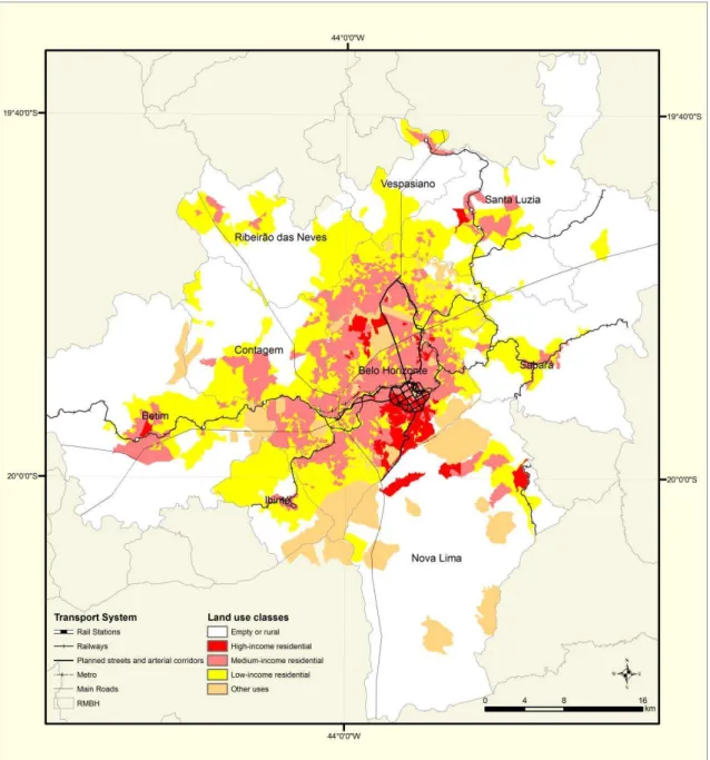
For the year 2000, the RMBH presents the numbers shown in Table 6. For the average-income class the patch size is much larger than that
for the high-income ones. Consequently, the perimeter and shape index are so as well. Further, the patch size for the average-income confirms its level of aggregation.
Figure 4 - Spatial distribution of land-use classes in year 2000
Table 6 - Basic measures of map – year 2000
High-income Average-income Low-income Global
Fractal dimension 1,334 1,429 1,386 1,397
Patch size 1751 14290 12819 12624
Perimeter 669 4985 3204 3651
Description of evolution from 1991 to
2000
In order to describe the evolution of the spatial occupation for the year 2000, the maps of differences among the different income-levels are presented in this section. The results are produced with a simple superposition of Figure 3 and Figure 4 using The Map Comparison Kit (VISSER; NIJS, 2006).
Large part of the difference observed is due to the increase of the population. The number of inhabitants increases 22%, from 3,212,044 in 1991 to 3,904,172 in 2000.
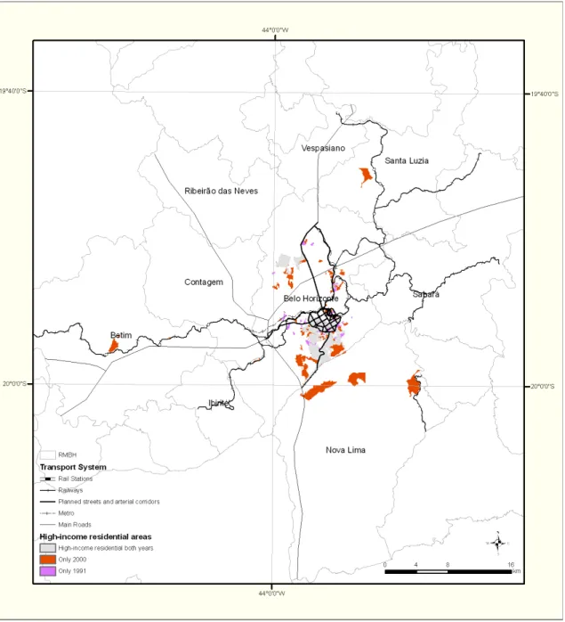
Figure 5 depicts the change of occupation of high-income residential areas and highlights their decentralization. Although maintaining the core upper-income areas southern of the central ring, further occupation is observed towards the so-called south-expansion vector (COSTA et al.,
2006) in the municipality of Nova Lima; in Belo Horizonte on the eastern area around a large shopping centre and western, near the Federal University campus. The central parts of Betim, Santa Luzia and Nova Lima also present newer areas of occupation indicating the upwards trend of some average-income locations into higher ones.
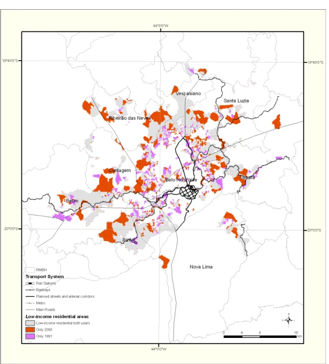
Figure 6 - Evolution of occupation of low-income residential areas from 1991 to 2000
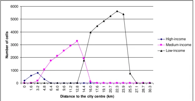
The change of occupation of low-income areas is shown in Figure 6. It confirms the decentralization along with physical expansion of the city, which is mostly taken by families with lower income. This decentralization is confirmed by the radial analysis (Figure 7 and Figure 9) which indicates that half of the occupation of low-income residential areas is accumulated at 14.4 km from the city centre in 1991, compared to 15.5 km in 2000.
Quantitative occupation of space by
different land-use classes
The calculus of how many cells is assigned for each class enables the analysis of how much space
is occupied by each income-level. This approach adds to the percentage analysis that considers domiciles for large aggregate areas.
In this paper, the same database and a similar aggregation of income-level8 is used to produce
the results in Table 7. The results 7 indicate that the numbers for general percentage analysis and spatial analysis are comparable. However, for average-income households – which increase in number proportionally (8 percentage points) – the
8 High-income refers to those domiciles with more than 20
physical occupation is slightly reduced. For low-income domiciles, the result is nearly the opposite. Although proportionally the number of families in this segment is reduced, the occupation is practically stable. Together, those effects might suggest that low-income families are occupying less dense areas in the outer borders of the metropolitan urban area. This is a similar result indicated by the visual analysis.
Distance to the CBD analysis
As mentioned in the introduction, the spatial distribution of income-level categories enables the comparison with general urban economics which
emphasizes mainly on „distance to the Centre Business District (CBD)‟ and „cost of transport‟.
In order to quantify the presence of different actors in relation to the city centre, a radial analysis is conducted (Figure 7). It measures the number of cells for every 20-cell large ring (annulus) with an initial position at the city centre9.
The results (Figure 7) suggest that, in general, urban economics principles hold. That is, poorer residents tend to locate farther from the centre, average-income households are half-way from the CBD, and higher-income people locate themselves closer to the centre. However, if the analysis is made in a finer scale, the configuration presents much less defined distinctions:
(a) in the first 10 km radius all three categories of income are present;
(b) the nearest to the CBD area is not exclusive of high-income occupation;
(c) the overlapping of land uses is continuous; and
(d) at 9 km, the number of domiciles for high-income is the same for the 4 km range which suggests multinodal configurations.
Table 7 - Quantitative occupation of space by different land-use classes
Spatial Analysis
Year 1991 Year 2000
Number of cells Number of cells
(absolute) Percentage (%) (absolute) Percentage (%)
High-income 3321 0.04 5850 0.06
Avdrage-income 27164 0.36 34672 0.34
Low-income 44198 0.69 55612 0.60
Total 74683 1.00 93134 1.00
Percentage analysus (a-spatial)
Year 1991 Year 2000
High-income 0.04 0.06
Avdrage-income 0.33 0.41
Low-income 0.63 0.53
0 1000 2000 3000 4000 5000
0.0 2.1 4.1 6.2 8.3 10.3 12.4 14.4 16.5 18.6 20.6 22.7 24.8 26.8 28.9 31.0 33.0 35.1
Distance to city centre (km)
N
um
be
r
of
c
e
ll
s
High-income Medium-income Low-income
Figure 7 - Radial distribute on of land-use classes from the city centre – year 19919
0 1000 2000 3000 4000 5000 6000 0 1
.6 3.2 4.8 6.4 8.0 9.6
1 1 .2 1 2 .8 1 4 .4 1 6 .0 1 7 .6 1 9 .1 2 0 .7 2 2 .3 2 3 .9 2 5 .5 2 7 .1 2 8 .7 3 0 .3
Distance to the city centre (km)
N um be r of c e ll s High-income Medium-income Low-income
Figure 8 - Radial distribution of land-use classes from the city centre – stylized city based on Lucas 2002 0 1000 2000 3000 4000 5000 6000
0.0 2.1 4.1 6.2 8.3 10.3 12.4 14.4 16.5 18.6 20.6 22.7 24.8 26.8 28.9 31.0 33.0 35.1
Distance to city centre (km)
N um be r of c e ll s High-income Medium-income Low-income
Figure 9 - Radial distribution of land-use classes from the city centre – year 2000
A similar exercise based on Lucas (2002) is made with stylized urban economics city (Figure 8) so that it can be used as a parameter of reference when analyzing the actual case.
The comparison between Figure 7 and Figure 8 confirms that they might look similar as Urban Economics suggest. But there are relevant differences in a closer look. The actual configuration presents much less defined distinctions with a relevant mix of presence of different groups within a 10 km radius.
The results for the distance to the CBD (Figure 7) confirm the suggestions made for 1991 (Figure 4).
Discussions
The results of this section can be summarized as follows. First, the clustering of income data from ten layers into three homogeneous income classes guided by the trained samples is presented for both years 1991 and 2000. In general, both maps show a non-linear urban space where income classes are definitely clustered together in clearly divided urban spaces. However, their boundaries are convoluted and there are intersections among all three classes independently of distance to the city centre. The analysis of the differences between the produced maps show in turn that although most of the land use classes remain in place throughout the decade, a clear path southwards of higher income within the Metropolitan Area of Belo Horizonte is noticeable. For the low-income residential areas, however, a general suburbanization stands out. Not a sprawl towards green areas and comfortable detached housing, but one that decreases mobility and accessibility to the job and service markets. In the case of low income sprawl, there is no defined direction with spread in all quadrants and in varied clustered sizes. Even if a periferization of low-income classes can be seen, the analysis of the quantitative occupation of income classes within the whole of urban space demonstrates that low-income residential areas have actually decreased as a proportion in the ten-year period analyzed. Finally, a parallel analysis made possible from the data produced is that one can test the regularities of spatial distribution predicted by the theory, as proposed by Lucas (2002), against actual observed occupation of urban space. The results prove by a large margin that although the theory holds if viewed from a very general perspective, it does not if an intraurban scale of analysis is used, such as in the case put forward by this paper.
Concluding remarks
This paper urges for the use of socioeconomically differentiated land-use classes to be applied into cellular automata (CA) models of urban development. It argues that contemporary cities are, by and large, too heterogeneous to be depicted in these models as single, urban residential class. The continuing overly-simplified use of automatic land-use classes provided by remote sensing might impair the scope of a field that is otherwise rich in providing urban development insights. Furthermore, it demonstrates that the use of georeferenced, detailed, socioeconomic data may add considerably to qualitative understanding of urban areas.
The empirical results contain spatially detailed analysis of Belo Horizonte and its Metropolitan region. Previous works were a-spatially explicit (MONTE-MÓR, 1994), used different structure (MENDONÇA, 2002), were restricted to the city of Belo Horizonte and used less detailed information (aggregated units) (PINHEIRO, 2006; PLAMBEL, 1987; SANTIAGO, 2006). The use of information at the scale of census tract allows for strengthened results with high degree of spatial confidence, which are in accordance, but further enhances more general results published earlier (MENDONÇA, 2002). These contributions together help the science field of built environment in general and urban public policies in specific to subsidize its studies making use of more precise and quantitative data, thus providing users with a more consistent array of analytical material. In conclusion, this paper provides:
(a) land-use classification that is useful as reference and validation data for CA models; (b) it demonstrates how quantitative exercises may be enlightening to qualitative analysis and description of urban environment;
(c) it illustrates how physical occupation of domiciles classified by income-level may vary differently from their proportion in the city in general; and
(d) finally, this paper might be helpful to validate
or reject urban economics models‟ spatial
configuration.
The simplicity of the analysis performed makes it easy to establish comparative studies, within Brazilian cities, or worldwide. This might portrait a more precise picture of spatial occupation of land-uses given by socioeconomic parameters.
References
ALLEN, P. M. Cities and Regions as
Self-Organizing Systems: models of complexity.
Amsterdam, Netherlands: Taylor & Francis, 1997. ALONSO, W. Location and Land Use: toward a
general theory of land rent. Cambridge, MA: Harvard University Press, 1964.
ARTHUR, B. Inductive Reasoning and Bounded Rationality. The American Economic Review, v.
84, n. 2, p. 406-411, 1994.
BATTY, M. Agents, Cells and Cities; new representational models for simulating multiscale urban dynamics. Environment and Planning A,
BATTY, M. Urban Evolution on the Desktop: simulation with the use of extended cellular automata. Environment and Planning A, v. 30, n.
11, p. 1943-1967, 1998.
BATTY, M. Cities and Complexity:
understanding cities with cellular automata, agent-based models and fractals. Cambridge, MA: The MIT Press, 2005b.
BATTY, M.; LONGLEY, P. Fractal Cities: a
geometry of form and function: Academic Press, 1994.
BENENSON, I.; TORRENS, P. M.
Geosimulation: automata-based modeling of
urban phenomena. London: John Wiley, 2004. BENENSON, I. et al. Geographic Automata
Systems and the OBEUS Software For Their Implementation. In: PORTUGALI, J. Complex
Artificial Environments. Amsterdam,
Netherlands: Springer Berlin Heidelberg, 2006. p. 137-153.
BERLEKAMP, E. R. et al.Winning Ways for
Your Mathematical Plays. Wellesley, MA: A K
Peters Ltd., 2004.
BOURASSA, S. C. et al. Defining Housing
Submarkets. Journal of Housing Economics, v.
8, n. 2, p.160-83, 1999.
BROWN, D. G. et al. Path Dependence and the
Validation of Agent-Based Spatial Models of Land Use. International Journal of Geographical
Information System, v. 19, n. 2, p.153-174, 2005.
CAPELLO, R.; NIJKAMP, P. (Eds.). Urban
Dynamics and Growth: advances in urban
economics. Amsterdam: Elsevier, 2004.
CLARKE, K. C. et al. A Self-Modifying Cellular
Automaton Model of Historical Urbanization in the San Francisco Bay area. Environment and
Planning B: Planning and Design v. 24, n. 2, p.
247–261, 1997.
COSTA, H. et al.Novas Periferias
Metropolitanas: a expansão metropolitana em
Belo Horizonte. Belo Horizonte, Brazil: C/Arte, 2006.
ENGELEN, G. et al.Report2550016006/2005.
Environmental Planning Agency Bilthoven, The Netherlands, 2005
ESRI. ArcMAP Desktop Help [Software].
Redlands, CA: ESRI Press, 2006.
FERNANDEZ, L. et al. Characterizing Location
Preferences in an Exurban Population: implications for agent-based modeling.
Environment and Planning B, v. 32, n. 6,
p.799-820, 2005.
GARDNER, M. Mathematical Games: the fantastic combinations of John Conway's new solitaire game 'Life'. Scientific American, v. 223,
n. 4, p.120-123, 1970.
HAGEN-ZANKER, A. Map Comparison Methods that Simultaneously Address Overlap and
Structure. Journal of Geographical Systems, v.
8, p.165–185, 2006.
HAGEN-ZANKER, A. et al. Measuring
Performance of Land Use Models. In: European Colloquium on Theoretical and Quantitative Geography, 14., Tomar, Portugal, 2005.
Proceedings… Tomar, Portugal, 2005. 11 p. HAGOORT, M. J. The Neighbourhood Rules:
land-use interactions, urban dynamics and cellular automata modelling. Utrecht, Netherlands: Faculteit Geowetenschappen Universiteit Utrecht, 2006.
HARDMAN, A.; IOANNIDES, Y. M. Neighbors' Income Distribution: economic segregation and mixing in US urban neighborhoods. Journal of
Housing Economics, v. 13, p. 368-82, 2003.
HOLLAND, J. Complex Adaptive Systems.
Daedalus, v. 121, n. 1, p.17-30, 1992.
HUBACEK, K.; BERGH, J. C. J. M. Changing Concepts of 'Land' in Economic Theory: from single to multi-disciplinary approaches. Ecological
Economics, v. 56, p.5-27, 2006.
INSTITUTO BRASILEIRO DE GEOGRAFIA E ESTATÍSTICA. Censo Demográfico 1991:
agregado por setores censitários dos resultados do universo. Brasília, Brazil: Ministério do
Planejamento/Instituto Brasileiro de Geografia e Estatística (IBGE), 1991.
INSTITUTO BRASILEIRO DE GEOGRAFIA E ESTATÍSTICA. Censo Demográfico 2000:
agregado por setores censitários dos resultados do universo. Brasília, Brazil: Instituto Brasileiro de Geografia e Estatística (IBGE), 2003.
LILLESAND, T. M. et al.Remote Sensing and
Image Interpretation. New York: Wiley, 2004.
LUCAS, R.; ROSSI-HANSBERG, E. On the Internal Structure of Cities. Econometrica, v. 70,
n. 4, p. 1445-176, jul. 2002.
MCGARIGAL, K. et al.FRAGSTATS: spatial
pattern analysis program for categorical maps [Software]. Amherst, MA: University of Massachusetts, 2002.
MENDONÇA, J. G. Segregação e Mobilidade
Residencial na RMBH. Rio de Janeiro, Brazil:
MENG, G. et al. Multi-Group Segregation Indices
for Measuring Ordinal Classes. Computers,
Environment and Urban Systems, v. 30, n. 3, p.
275-299, 2006.
MONTE-MÓR, R. L. Belo Horizonte: espaços e
tempos em construção. Belo Horizonte: CEDEPLAR/PBH, 1994.
PINHEIRO, F. J. Desenvolvimento Humano na
Região Metropolitana de Belo Horizonte: atlas
metropolitano. Belo Horizonte: Centro de Estudos Econômicos e Sociais, Fundação João Pinheiro, 2006.
PLAMBEL. O Mercado da Terra na Região
Metropolitana de Belo Horizonte. Belo
Horizonte: Plambel, 1987.
PONTIUS, R. et al. Comparing the Input, Output,
and Validation Maps for Several Models of Land Change. The Annals of Regional Science, v. 42,
n. 1, p. 11-37, 2008.
PORTUGALI, J. Self-Organization and the City.
Berlin: Springer-Verlag, 2000.
RIKS. Map Comparison Kit 3: user manual.
Maastricht, Netherlands: RIKS BV, 2006. SANTIAGO, R. Obsolescência Programada no
Mercado Imobiliário: o espaço como forma de
entesouramento. Belo Horizonte, Brazil: Escola de Arquitetura/UFMG, 2006.
SCHELLING, T. C. Micromotives and
Macrobehavior. New York, London: W W
Norton & Co Ltd, 1978.
SILVA, E. A.; CLARKE, K. C. Calibration of the SLEUTH Urban Growth Model for Lisbon and Porto, Portugal. Computers, Environment and
Urban Systems, v. 26, p.525-252, 2002.
SIMÕES, R. F. Localização Industrial e
Relações Intersetoriais: uma análise de fuzzy
cluster para Minas Gerais. Campinas, Brazil: Instituto de Economia/Unicamp, 2003.
SIMÕES, R. F. Localização Industrial e
Relações Intersetoriais: uma análise de fuzzy
cluster para Minas Gerais. Campinas: Instituto de Economia/Unicamp, 2003.
SIMÕES, R. F. Métodos de Análise Regional e
Urbana: diagnóstico aplicado ao planejamento.
Belo Horizonte, Brazil: CEDEPLAR/UFMG, 2005.
SOJA, E. W. Postmetropolis: critical studies of
cities and regions. Malden, MA: Blackwell Publishers, 2000.
THÜNEN, J. H. Der isolierte Staat. New York:
Pergamon Press, 1966.
VISSER, H.; NIJS, T. The Map Comparison Kit.
Environmental Modeling & Software, v. 21, n.
3, p. 346-358, 2006.
WADDELL, P.; ULFARSSON, G. F. Dynamic Simulation of Real Estate Development and Land Prices Within an Integrated Land Use and Transportation Model System. In:
TRANSPORTATION RESEARCH BOARD ANNUAL MEETING, 82., Washington, D.C., 2003. Proceedings…, Washington, D. C., 2003. WADDELL, P. et al. Incorporating Land Use in
Metropolitan Transportation Planning.
Transportation Research, v. 41, p.382-410,
2007.
WHITE, R.; ENGELEN, G. Cellular Automata and Fractal Urban Form: a cellular modelling approach to the evolution of urban land-use patterns. Environment and Planning A, v. 25, n.,
p. 1175-1199, 1993.
Revista Ambiente Construído
Associação Nacional de Tecnologia do Ambiente Construído Av. Osvaldo Aranha, 99 - 3º andar, Centro
Porto Alegre – RS - Brasil CEP 90035-190 Telefone: +55 (51) 3308-4084
Fax: +55 (51) 3308-4054 www.seer.ufrgs.br/ambienteconstruido