Analysing Data of the Integrated Administration and Control System (IACS) to Detect Patterns of Agricultural Land-Use Change at Municipality Level

(1)

*Corresponding author nicola.lueker-jans@umwelt.uni-giessen.de

© The Authors. 2016. Landscape Online. This is an Open Access aricle distributed under the terms of the Creaive Commons Atribuion License (htp://creaivecommons.org/licenses/by/4.0), which permits unrestricted use, distribuion, and reproducion in any medium, provided the original work is properly cited.

ISSN 1865-1542 – www.landscapeonline.de – htp://dx.doi.org/10.3097/LO.201648 LANDSCAPE ONLINE 48:1-24 (2016), DOI 10.3097/LO.201648

Nicola Lüker-Jans

1

*, Dietmar Simmering

2

, Annette Otte

1

1 Justus-Liebig-University Giessen, Division of Landscape Ecology and Landscape Planning, Heinrich-Buff-Ring 26-32; D-35392

Giessen

2 Ingenieurbüro für Umweltplanung Dr. J. Karl, Staufenberger Straße 67; D-35460 Staufenberg

Abstract

European landscapes have featured considerable changes towards intensification and marginalisation. These major trends are expected to continue in the future. Besides, the cultivation of bioenergy crops has become an important factor in agricultural land use. A thorough understanding of land-use processes for management purposes is needed. In this study, the spatial and temporal pattern of agricultural land use and land-use change was classified at the scale of municipalities from 2005 to 2010. The study region was the German federal state Hesse. By using data of the Integrated Administration and Control System (IACS) of the European Union and with the help of k-means cluster analysis, five types of agricultural land-use patterns and dynamics (TLPDs) were detected. These TLPDs represent different sub-regions. Sub-regions with favourable physical conditions for cultivation are dominated by arable land. A progressive land-use change occurred by conversion of grassland to arable land. In sub-regions, where physical conditions are rather unfavourable, especially in mountainous areas, grassland is the predominant land use. But on the remaining arable land, there is a slight change in favour of maize. The knowledge of sub-regions with spatially and temporally different agricultural land use could be utilised to develop land management instruments like site-specific agri-environmental schemes.

Keywords:

land-use data set, classification, cluster analysis, identification of sub-regions, agri-environmental schemes, Germany

Submitted: 22 October 2015 / Accepted in revised form: 27 February 2016 / Published: 22 March 2016

(2)

ISSN 1865-1542 - www.landscape-online.de

Oicial Journal of the Internaional Associaion for Landscape Ecology – Regional Chapter Germany (IALE-D)

1 Introduction

L

and use is a central component of the landscape

that surrounds us. Changes in land use and land cover are influenced by both human activities and several natural ecological processes, and vary across space and time (Petit & Lambin 2002; Verburg et al. 2010). Land cover refers to biophysical attributes (either of natural or anthropogenic origin) of the

earth’s surface and immediate subsurface. Land use

refers to human activities that exploit the land cover with the purpose of producing goods and services (Lambin et al. 2000; de Chazal & Rounsevell 2009).

This paper focusses on agricultural land use. Many

studies have analysed the dynamics of agricultural land use since it became evident that these dynamics affect the environment (Bürgi et al. 2004), ecosystem functioning, and natural resources like water and soil quality, habitat quality, species richness, biodiversity, and others (Vagstad & Oygarden 2003; Rounsevell et al. 2006; Xiao et al. 2006).

In the last several decades, in Europe two opposing trends can be identified in agricultural land use: intensification and marginalisation (Stoate et al. 2009). Agricultural intensification, characterised by both a comparatively higher output of cultivated products per unit area and time, and a higher level of inputs like agrochemicals (Lambin et al. 2001), has been driven by market demands and agricultural policies with the aim of an increased production and efficiency. Hence, intensive land use is connected to landscapes with rather favourable site conditions for arable cultivation like relatively flat and fertile land. The intensification processes in these regions have caused enlarged field sizes, a removal of boundary vegetation as well as a less diversified crop rotation (Fjellstad & Dramstad 1999). In contrast, landscapes affected by marginalisation are characterised by steep slopes, shallow and/or poor soils and an inferior accessibility. Thus, the process of marginalisation can be found especially in mountain regions (MacDonald et al. 2000). Marginal agricultural landscapes are often characterised by an increased biodiversity and habitat richness due to low intensities of cultivation, crop and grassland rotation, small-parcelled mosaics etc. In these landscapes for about six decades,

large portions of arable land have been replaced by plantation forestry, rotational fallows and especially by extensive grassland, so that landscape structure has considerably changed (Waldhardt & Otte 2003). Meanwhile, due to increasingly unfavourable economic conditions these landscapes are in danger of undergoing distinct changes by either abandonment or intensification of the remaining agricultural area (Meeus 1995; Harvolk et al. 2013). Thus, management is needed in order to preserve marginal agricultural landscapes (Waldhardt et al. 2004).

(3)

Finally, since the second half of the twentieth century, agricultural land use in Europe has undergone major changes due to technological advances, urban expansion, market conditions, globalisation, enlargement of the EU and the Common Agricultural Policy (CAP). Given this background, European land use is likely to experience ongoing changes in the future (Rounsevell et al. 2003; Keenleyside et al. 2009; Sanderson et al. 2013). Hence, a thorough understanding of past and recent land-use processes is essential in order to understand how agricultural land use might develop in the future.

The EU is well aware of the impact of the CAP on agricultural land use. By supporting the agricultural sector mainly through transfer payments, the CAP is a strong determining factor (Heißenhuber & Krämer 2011). Transfer payments are divided into direct support payments which all farmers receive per ha of farmland, i.e. an area payment, and agri-environmental payments which are offered if farmers voluntarily obligate themselves to comply with an ecologically beneficial cultivation and/or animal husbandry (Reger et al. 2009b). By giving these payments, farmers can be influenced in their management decisions. Thus, the CAP is an important driver of changes in agricultural land use (Strijker 2005). For specific background to the CAP see for example Erjavec & Erjavec (2015) and Gomez y Paloma et al. (2013). As well as income and risk coverage of the EU’s farmers, another important aim of the CAP is to consider environmental issues. In this context, direct support payments are coupled to environmental and further standards what means that farmers only get the payments in full if they comply with these standards. One of the environmental aims of the CAP is the protection of permanent grassland. In the past, EU member states had to ensure that the conversion of permanent grassland must not exceed a 10% threshold, i.e. the ratio of permanent grassland in relation to the total agricultural area must not decrease by more than 10% referred to the year 2003 (according to Regulation (EC) No 796/2004). But most of the member states applied stricter rules. However, with the latest reform of the CAP, the 10%-requirement for reduction in permanent grassland was tightened. Since 2015, the ratio of permanent grassland in

relation to the total agricultural area must not be reduced by more than 5%, but referred to the year 2012 (according to Regulation (EU) No 1307/2013) rather than 2003. Member states of the EU had, and still have, to monitor this requirement. Usually, the spatial basis is at the national level. In Germany, the monitoring of permanent grassland is performed at the level of the federal states which reflects the regional level within the EU (Nitsch et al. 2012). Furthermore, the federal states are also the spatial unit for offering different agri-environmental schemes. But this spatial level may hide differences of land-use patterns within the federal states, i.e. at sub-regional level.

(4)

payments are carried out accurately, that controls are implemented, and that amounts unduly paid are recovered. Fulfilling these purposes, the Integrated Administration and Control System (IACS) was implemented by regional authorities (EC 2013). Since 2004, in order to achieve direct support payments, farmers have had to register all agricultural parcels of land and the cultivated crops every year. As a result, IACS data provide information on land use at the field level on an annual basis as well as information on field size, farm type, legal structure, livestock etc. Thus, IACS data provide a promising data set for analysing agricultural land use and land-use change. However, until now studies using IACS data are scarce, but see Nitsch et al.(2012), Harvolk et al. (2013), de Longueville et al. (2007), Trubins (2013), who analysed land use and land-use change processes down to field level or used the IACS parcel plan for their studies.

In this study, we developed a classification method to detect spatial and temporal differences of patterns of agricultural land use at sub-regional level which is based on a solid quantitative data source. Further, we were interested to answer the following questions: Which types of land-use patterns could be identified in the study region? Which areas experienced major, minor or no changes of agricultural land use in recent years? Which areas are probably sensitive to future land-use changes and in what manner? The study region was Hesse, one of the federal states in Germany. Hesse was chosen due to its various biogeographical regions comprising both marginal and intensively used agricultural landscapes. By using data of the Integrated Administration and Control System (IACS), we collected information on agricultural land use for the years from 2005 to 2010 and analysed the data at the municipality level (which is the LAU level 2, i.e. the lower level of the officially defined Local Administrative Units within the EU).

Building upon Reger et al. (2007), who studied past land-use change, the aims of the study were:

(i) to identify ‘types of agricultural land-use patterns and dynamics (TLPDs)’ at the scale of municipalities for the time period 2005 to 2010, and

(ii) to characterise the identified types by using physical landscape attributes (elevation, slope, temperature and precipitation) and the intensity of livestock farming (expressed by livestock data, i.e. cattle and pig numbers, and a livestock density index).

2 Study region

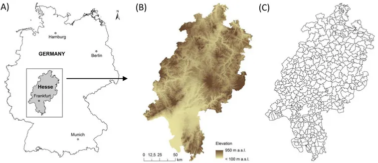
T

he German federal state Hesse (Figure 1) is

located in central Germany and comprises 430 municipalities. Hesse covers 21.115 km², the maximum north-south extent amounts to 250 km and the maximum east-west extent to 170 km (HSL 2012).

In Hesse, there is a variety of different landscapes (Pletsch 1989). Hesse is part of the central German mountain threshold which is characterised by a spatial alternation of valleys (< 300 m a.s.l., planar to colline altitude level) and mountain ranges (> 300 m a.s.l., submontane to montane altitude level). This large-scale pattern stretches in a more or less north-south direction. The highest point lies in the eastern low mountain range, called Rhön (950 m a.s.l.). The valleys of the rivers Rhine and Main in the south are the lowest points (< 100-200 m a.s.l.) (Jungmann & Brückner 2005).

The four main biogeographical regions are (i) Rhenish Slate Mountains (Rheinisches Schiefergebirge), (ii) West Hessian Highlands and West Hessian

Depression (Westhessisches Bergland und

Westhessische Senke), (iii) East Hessian Highlands and East Hessian Depression (Osthessisches Bergland und Osthessische Senke) and (iv) South Hessian Valleys and Elevations (Südhessische Becken- und Gebirgsländer) (Meynen & Schmithüsen 1953-1962; Klausing 1988; Pletsch 1989).

(5)

brown soils and pararendzina soils. On calcareous windborne sands luvisols and black earth soils are prevailing (Sabel 2005).

Hesse lies in the zone of the warm temperate, rainy climate of the middle latitudes. But the regional climate is characterised by a variety of different climate conditions which can be explained by the orographic heterogeneity (Pletsch 1989). The lowlands are notably warm (mean annual temperature: 9-10° C), for example in the Rhine-Main area. In contrast, the highlands are notably cold (mean annual temperature: 5° C). The mean annual precipitation (1971-2000) varies between 500 mm in the south-west of Hesse and 1,200-1,300 mm in the north-western highlands (Mollenhauer 2005).

Land use in Hesse is presented in Table 1. For reason

of comparison, land use of Germany as a whole is shown, too. In Hesse, agricultural land use varies between the different landscapes. For example, in the Rhine-Main lowlands land use is characterised by intensive arable farming due to favourable physical conditions like humous soils and the warm climate. Here, the dominant crops are vegetables and sugar beets. Field irrigation is often applied. In some cases, where soils are sandy and nutrient-poor, extensive forest areas appear and asparagus is grown. In the fertile loess areas, mostly wheat, sugar beets, rape seed and barley are grown, in some cases also vines and fruits. In the low mountain ranges and hilly landscapes, there is a mixture between agriculture, forestry and grassland which is dependant on soil quality, relief and climate. Thus, land use is less intensive. Many of these regions belong to the less favoured areas (Harrach 2005).

Table 1: Land use in Hesse (HMUELV 2011; HSL 2012) and Germany (DBV 2010; 2012) in 2010

Land use Proportion of utilised agricultural

land

Agriculture

(%) Forestry (%) Settlement and traffic (%)

Arable land

(%) Grassland (%)

Hesse 42 40 16 62 37

Germany 52 30 14 71 29

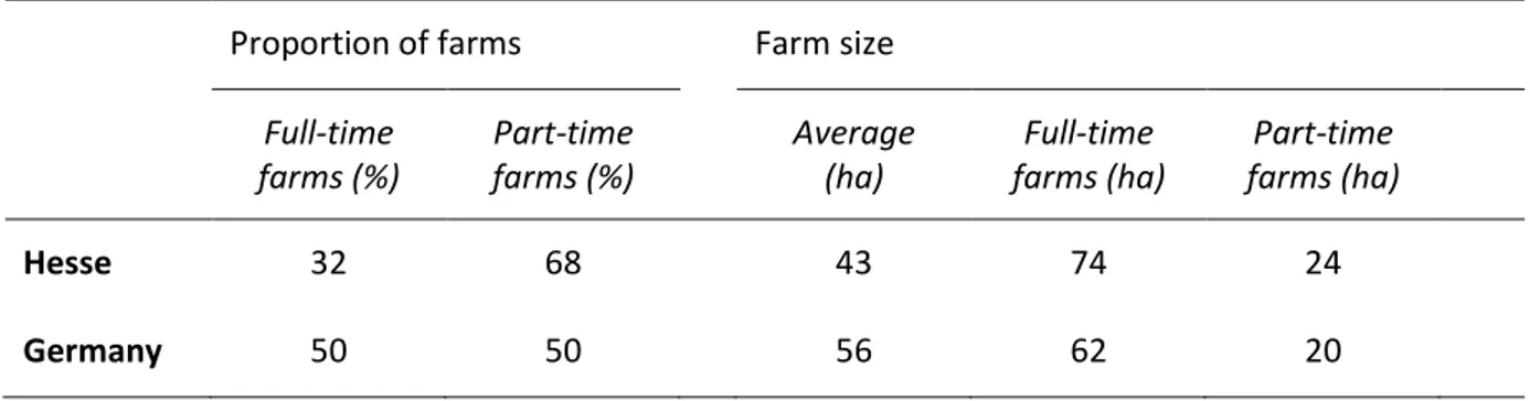
Table 2: Farm structure in Hesse (HMUELV 2011; HSL 2012) and Germany (DBV 2012) in 2010

Proportion of farms Farm size

Full-time

farms (%) Part-time farms (%) Average (ha) farms (ha)Full-time farms (ha)Part-time

Hesse 32 68 43 74 24

Germany 50 50 56 62 20

Table 1: Land use in Hesse (HMUELV 2011; HSL 2012) and Germany (DBV 2010; 2012) in 2010

(6)

In Hesse livestock farming is an important component of agriculture. Nevertheless, pig and cattle stocks are decreasing. In 2010, total livestock comprised 469.750 livestock units (LU), on an average 0.6 LU per ha utilised agricultural land (in Germany: 1.1 LU/ ha on average). Livestock farming is concentrated in the north and the east of Hesse (HMUELV 2011).

Table 2 shows the structure of the Hessian and, for reasons of comparison, of the German farms. Traditionally, Hesse has been the land of a rather small-scale agriculture, especially in the middle and in the south. Currently, the number of farms is still

decreasing and their land is absorbed by the growing farms. Thus, the average farm size increased from 26 to 43 ha between 1999 and 2010 (HMUELV 2011).

Owing to relief, climate and soil conditions, the study region Hesse is characterised by a steep gradient of potential agricultural land use comprising marginal agricultural landscapes of the highlands, intensively used agricultural landscapes of the lowlands and a mixture of them. Thus, characterised by areas favourable as well as unfavourable for agricultural use, Hesse is most suitable for analysing types of land use differing in the spatial and temporal pattern.

*Corresponding author. Email: nicola.lueker-jans@umwelt.uni-giessen.de

© The Authors. 2013. Published by Landscape Online, IALE-D. This is an Open Access article distributed under the terms of the Creative Commons Attribution License (http://creativecommons.org/licenses/by/3.0), which permits unrestricted use, distribution, and reproduction in any medium, provided the original work is properly cited.

ISSN 1865-1542 – www.landscape-online.de – http://dx.doi.org/10.3097/LO.201333

Page 1

1

2 3 4 5 6 7 8 9 10 11 12 13

Figure 1: Study area: (A) Hesse in Germany, (B) topography (elevation between < 100 and 950 m a.s.l)

14

(Jungmann and Brückner 2005), (C) 430 municipalities (HSL 2012)

15

16 17

(A) (B) (C)

3 Methods

3.1 Data set of the Integrated Administration and Control System (IACS)

The main data used for the analyses were digital polygonal layers of land use at the field level as provided by the Integrated Administration and Control System (IACS). We used IACS data of Hesse for the years from 2005 to 2010, made available for this study by the Hessian Agency for Environment

and Geology (HLUG undated). Generally, IACS data are not freely available.

The IACS data set for the Hessian state contained one GIS polygon layer for each year that featured all registered agricultural fields and their land use in the respective year. This layer was intersected with the boundaries of the 430 municipalities, the spatial basis of the study. The boundaries of the Hessian municipalities were provided by the German Federal Office for Cartography and Geodesy (BKG 2011). Land use was grouped according to the land-use

(7)

classes of the IACS data set: arable land, permanent grassland, permanent crops and non-agricultural area. The sum of the areas of these four land-use classes represents the total utilised agricultural land in each of the municipalities. However, the total area of utilised agricultural land of the municipalities differed considerably between the years 2005 to 2010 irrespective of the area of the municipality. A preceding analysis of the data had revealed this fact, i.e. we identified for each municipality the maximum and the minimum areas of utilised agricultural land which was registered in any one of the years between 2005 and 2010. Then, we calculated the ratio of the difference between the maximum and the minimum area of utilised agricultural land in relation to the maximum agricultural land for each municipality. On average, this ratio was 4.9%. The reason for this variability is that farmers are not obliged to declare their fields for direct support payments, although these fields are still cultivated. If farmers decide not to declare, the fields will not be included in IACS data. As a consequence for the analysis, in order to get a consistent reference value, we decided to take the maximum area of agricultural land and of arable land for each municipality. These maximum areas were assumed as the available areas of utilised agricultural or arable land in the respective municipality.

Since we intended to classify the municipalities according to the patterns of agricultural land use and land-use change, we chose the following four variables (Table 3) based on the IACS data set and calculated them for all 430 municipalities. The aim was to consider variables of agricultural land use which reflect the recent and actual pattern as well as the most important dynamics of recent years. The first variable is calculated as (i) proportion of grassland in 2005 expressed as the percentage (%) of the (maximum) utilised agricultural land. This variable comprises the area of permanent grassland as defined in the IACS data, i.e. the sum of meadows, pasture land, 20-years land set-aside etc. The second and the third variable consider the cultivation of maize. Maize proved to be one of the crops with a strong increase in cultivation in recent years in Hesse. Thus, this crop was chosen to express

changing situations in agricultural production. The second variable is calculated as (ii) proportion of maize area in 2010 expressed as the percentage (%) of the (maximum) arable land. This variable comprises the sum of the area for grain-maize, corn-cob-mix, sweetcorn and silage maize. In this context, we did not know whether maize is used for bioenergy production or not, since IACS data do not provide this information. The third variable is calculated as (iii) expansion of maize area quantified as the average annual expansion rate as the percentage (%) for the proportion of maize area in the time period 2005 to 2010. The latter variable was quantified using the geometric mean, a quantity which calculates the average annual growth rates distributed equally to the respective years (Zeidler 2013), so that the different growth rates of the municipalities are suitable for comparison. Finally, the last variable considers conversion of grassland to arable land. Here, we calculated (iv) the conversion of grassland into arable land between 2005 and 2010 expressed as the percentage (%) of grassland area in 2005. As the protection of grassland against conversion into arable land or other agricultural uses, against loss or decline of its ecological functions is of high importance with respect to several environmental objectives, we included this variable in the study. We considered only the conversion of grassland into arable land, since this direction of conversion seems to be the most dominant (Nitsch et al. 2012).

In order to ensure that these four variables of agricultural land use are not interdependent, i.e. they do not correlate, correlation coefficients among the variables were calculated. The coefficients did not show any relationship between the variables (correlation coefficients between -0.1 and 0.2). Thus, we concluded that the variables are suitable for the analysis.

(8)

Oicial Journal of the Internaional Associaion for Landscape Ecology – Regional Chapter Germany (IALE-D) 3.2 Physical landscape attributes and livestock

numbers

Physical landscape attributes are known to be relevant determinants for agricultural land use and they correlate with land-use change processes (Pan et al. 1999; Schneider & Pontius 2001; Hietel et al. 2004). Hence, we selected four variables to describe the main environmental drivers for agricultural production: (i) elevation, (ii) slope, (iii) temperature, (iv) precipitation. For each municipality, the means of these variables were calculated.

Information on elevation and slope were derived from a digital elevation model (DEM, 25 m resolution), provided by the Hessian State Office for Land Management and Geoinformation (HVBG undated). The underlying raster data set of the DEM was used as the basis to calculate mean elevation (metre a.s.l.) and mean slope (°) within each municipality. Information on climate, with the variables temperature and precipitation, were made available in a 1 km²-resolution by the German Weather Service (DWD 2013). For each municipality,

we calculated the mean annual temperature (°C) and the mean annual precipitation (mm), both for the time period from 1981-2010.

The processing of physical landscape data was performed also with ArcGIS 10 using the Spatial Analyst tool (ESRI 2010).

To characterise the municipalities regarding the agricultural structure, we quantified livestock numbers. Livestock is known to be relevant for land use because of the fodder needs. Since the degree of self-sufficiency for fodder is very high (in 2010/2011: 89% for fodder corn in Germany), cultivation of fodder is an important part of land use (DBV 2012). Thus, changes in livestock are one reason of land-use changes (Hietel et al. 2007). Livestock data were collected using the Hessian agricultural statistics which is a data set providing detailed information on agriculture. In 2010, the agricultural structure survey (German: Agrarstrukturerhebung) was implemented, thus giving comprehensive and detailed information on agricultural land use. Based on the Hessian agricultural statistics (HSL 2012), for the year 2010 Table 3: Variables of agricultural land use used for k-means cluster analysis to detect types of

agricultural land-use patterns and dynamics (TLPDs)

Variable Description Aim

Grassland area, 2005 (% of util. agr. land) Proportion of grassland in 2005 as percentage of utilised agricultural land *

Description of status of land use at the beginning of the investigation time

Maize area, 2010 (% of arable land) Proportion of maize area in 2010 as percentage of arable land **

Description of status of land use at the end of the investigation time

Expansion of maize area, 2005-2010 (%) Average annual expansion rate as percentage for the proportion of maize area in the time period 2005-2010

Rating of land-use change for the entire time period of investigation

Conversion of grassland 2005 to arable land

2010 (% of grassland 2005) Grassland arable land between 2005 and converted into 2010, as percentage of grassland area in 2005

Rating of land-use change for the entire time period of investigation

* relating to the maximum area of utilised agricultural land from 2005-2010; ** relating to the maximum area of arable land from 2005-2010; see text for details

(9)

we got information on (i) the number of cattle, (ii) the number of pigs, and (iii) the livestock density index expressed as livestock unit per ha utilised agricultural land (LU/ha) (EC 2011). For reasons of data protection, the data were not available for all of the 430 municipalities. According to agricultural statistics, information on livestock is missing in the case if information could be assigned clearly to a single farm. Concerning the number of cattle, we got information for 384 municipalities, concerning pigs for 326 municipalities and concerning livestock density for 396 municipalities. Nevertheless, we used these data for the analysis. Since the missing data points on livestock are scattered all over Hesse, the data are still representative for the study area.

3.3 Statistical analysis

In this study, we performed a k-means cluster analysis, since we aimed to identify types of agricultural land-use patterns and dynamics (TLPDs). As a method of multivariate data analysis, cluster analysis proved to be a suitable method for analysing land-use change, see for example Mendoza et al. (2011), Potashev et al. (2014), Reger et al. (2007) and Stuczynski et al. (2003). The k-means cluster algorithm is a partitioning method (MacQueen 1967). It aims to identify groups or clusters in relatively unknown data sets whereupon the variability between the clusters is maximised and the variability within the clusters is minimised (Hartigan & Wong 1979). Thus, the homogeneity within the clusters allows to characterise these clusters, whereas the heterogeneity between the clusters causes a sharp partitioning (Hartigan 1975).

K-means cluster analysis was performed for the four selected variables of agricultural land use (see Table 3). The statistical process was to allocate the municipalities and accordingly the included variables to different clusters. For each cluster the centroids were defined, i.e. the arithmetic means for the four variables across the clusters were calculated. The k-means algorithm is based on minimising the sum of squared deviations to the centroids. As a result the centroids are as different from each other as

possible. For reasons of comparison, we tried also to consider more variables of agricultural land use. For example, the variables proportion of maize area in 2005 and proportion of grassland in 2010 were added. But k-means cluster analysis did not show useful results. Therefore, we chose the four variables as presented before.

In order to find the ‘best’ number of clusters, v-fold cross validation was performed (Janisová et al. 2014; Flanagan & Cerrato 2015; Gumienna et al. 2016). The benefit of v-fold cross validation is that the number of clusters will be determined from the data and must not be known a priori which means prior knowledge about the number of clusters is not essential. V-fold cross validation is an algorithm of repeated calculation. The purpose of this process is to divide the overall sample into a number of v folds (here: 10) which are subgroups (Hastie et al. 2009). One subgroup will be excluded in order to serve as a testing sample. Subsequently, the allocation of the samples to generate clusters will be performed without the testing sample. After the clusters are generated and the samples are allocated, the testing sample is also allocated to these clusters. In this test sample, an error rate will be calculated. The process is repeated according to the number of subgroups. With each repetition another subgroup is excluded and another error rate is determined. The number of clusters with the lowest error rate will be taken as final result.

Hence, in the analysis every cluster contains municipalities with similar characteristics, but well-contrasted to the others. Thus, the derived clusters represent the types of agricultural land-use patterns and dynamics (TLPDs) in Hesse.

(10)

significant differences between the derived TLPDs by using physical landscape attributes and livestock data. In case of significance, a Median-test for multiple testing (p < 0.05) followed.

For all analyses we used Statistica 10.0 software (StatSoft. Inc. 2011).

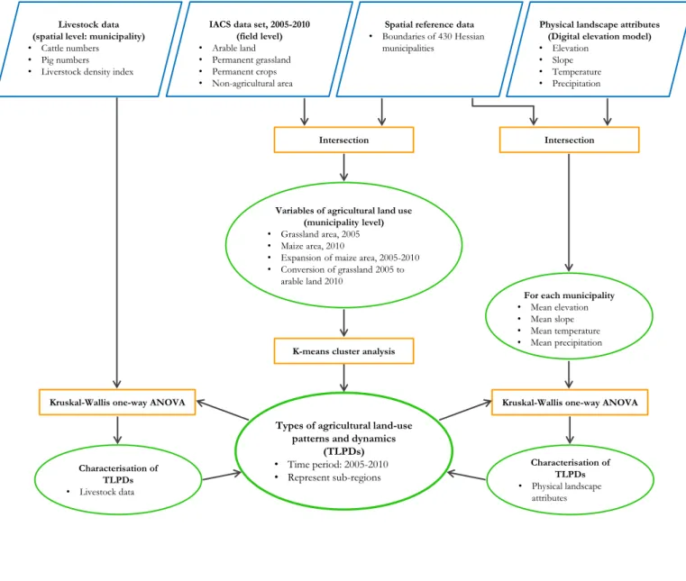
Figure 2 illustrates the work flow of the applied methodology.

Variables of agricultural land use (municipality level)

• Grassland area, 2005

• Maize area, 2010

• Expansion of maize area, 2005-2010

• Conversion of grassland 2005 to arable land 2010

For each municipality

• Mean elevation

• Mean slope

• Mean temperature

• Mean precipitation

Kruskal-Wallis one-way ANOVA

Intersection

K-means cluster analysis Intersection

Types of agricultural land-use patterns and dynamics

(TLPDs) • Time period: 2005-2010 • Represent sub-regions

Characterisation of TLPDs

• Physical landscape attributes

Kruskal-Wallis one-way ANOVA Physical landscape attributes

(Digital elevation model)

• Elevation

• Slope

• Temperature

• Precipitation

Livestock data (spatial level: municipality)

• Cattle numbers

• Pig numbers

• Liverstock density index

Spatial reference data

• Boundaries of 430 Hessian municipalities

IACS data set, 2005-2010 (field level)

• Arable land

• Permanent grassland

• Permanent crops

• Non-agricultural area

Characterisation of TLPDs

• Livestock data

Figure 2. Work flow of the applied methodology Input

data Method Output

(11)

4 Results

4.1 Types of agricultural land use patterns and dynamics

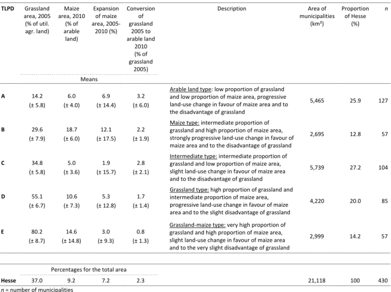
The k-means cluster analysis detected five different types of agricultural land-use patterns and dynamics (TLPD A-E, Table 4). They represent the different spatial and temporal patterns of land use and land-use change between the years 2005 to 2010 at the level of municipalities, i.e. at the sub-regional level. For a description of the main characteristics of the types A-E see Table 4, and Figure 3 for their spatial distribution.

TLPD A, the arable land type, ranges from north to south and lies mostly in the centre of Hesse, and thus,

represents the lowlands of the Hessian landscape (cf. Figure 1B). Consequently, the proportion of grassland in 2005 was low (14.2%). The proportion of maize area in 2010 was low (6.0%) as well. TLPD A municipalities are characterised by a progressive land-use change in favour of maize to the disadvantage of grassland which means a conversion of grassland. In TLPD B, the maize type, the proportion of maize in 2010 as well as the average annual expansion rate for maize between 2005 and 2010 were the highest of all TLPDs. The latter indicates that TLPD B experienced a distinctive land-use change between 2005 and 2010. The municipalities grouped in TLPD B are scattered throughout the entire study region, but do not occur in the highlands. In contrast, TLPD C, which is the intermediate type, is characterised by a low proportion of maize area (5.0%) and a low average annual expansion rate for maize (1.9%). But

LANDSCAPE ONLINE xx:1-xx (2013), DOI 10.3097/LO.2013xx

_{Page 2}

Official Journal of the International Association for Landscape Ecology – Regional Chapter Germany (IALE-D)

18 19 20 21 22 23 24 25 26 27 28 29 30 31 32 33 34 35 36 37

Figure 3: Spatial distribution…

38 39

TLPD A municipalities

TLPD B municipalities

TLPD C municipalities

TLPD D municipalities

TLPD E municipalities

(12)

the conversion of grassland to arable was the second highest of all clusters (2.8% from 2005 to 2010). TLPD D and E, the grassland and the grassland-maize type, are both dominated by grassland because of their location in the Hessian highlands. The proportion of grassland is traditionally high to very high. These types featured only a slight land-use change regarding grassland loss and maize expansion. However, they differ with respect to the proportion of maize cultivated on the limited arable land.

Despite these agricultural land-use patterns and dynamics at municipality level, we also detected land-use change processes for the entire study area. According to IACS data, in Hesse the proportion of grassland was intermediate (37.0%) in the year 2005

and remained almost stable with 36.5% in the year 2010. The conversion rate of grassland to arable land was 2.3% for the study period. On arable land, in the year 2005 6.5% were covered by maize. The average annual expansion rate for maize was 7.2% from 2005 to 2010 which resulted in an intermediate proportion of maize area (9.2%) in the year 2010.

4.2 Characterisation of types of agricultural land use patterns and dynamics (TLPDs) by physical landscape attributes and livestock numberss

The five identified TLPDs reveal distinct differences regarding the four physical landscape attributes (Table 5), which correspond with the variety of Hessian landscapes.

Table 4: Types of agricultural land-use patterns and dynamics (TLPD A-E) characterised by four land-use variables based on IACS data. Results of the k-means cluster analysis are means (with standard deviation). For reasons of comparison, land-use variables of Hesse as a whole are indicated in the last row.

TLPD Grassland area, 2005

(% of util. agr. land) Maize area, 2010 (% of arable land) Expansion of maize area, 2005-2010 (%) Conversion of grassland 2005 to arable land 2010 (% of grassland 2005)

Description Area of

municipalities (km²) Proportion of Hesse (%) n Means

A 14.2

(± 5.8) 6.0 (± 4.0) 6.9 (± 14.4) 3.2 (± 6.0)

Arable land type: low proportion of grassland and low proportion of maize area, progressive land-use change in favour of maize area and to the disadvantage of grassland

5,465 25.9 127

B 29.6

(± 7.9) 18.7 (± 6.0) 12.1 (± 17.5) 2.2 (± 1.9)

Maize type: intermediate proportion of grassland and high proportion of maize area, strongly progressive land-use change in favour of maize area and to the disadvantage of grassland

2,695 12.8 57

C 34.8

(± 5.8) 5.0 (± 3.6) 1.9 (± 15.7) 2.8 (± 2.1)

Intermediate type: intermediate proportion of grassland and low proportion of maize area, slight land-use change in favour of maize area and to the disadvantage of grassland

5,739 27.2 104

D 55.1

(± 6.7) 10.6 (± 7.3) 5.3 (± 12.8) 1.7 (± 1.4)

Grassland type: high proportion of grassland and intermediate proportion of maize area, progressive land-use change in favour of maize area and to the slight disadvantage of grassland

4,220 20.0 85

E 80.2

(± 8.7) 14.6 (± 14.8) 3.0 (± 9.3) 0.8 (± 1.3)

Grassland-maize type: very high proportion of grassland and high proportion of maize area, slight land-use change in favour of maize area and to the very slight disadvantage of grassland

2,999 14.2 57

Percentages for the total area

Hesse 37.0 9.2 7.2 2.3 21,118 100 430

(13)

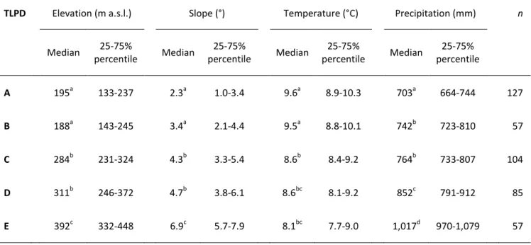
With low elevations, flat slopes and a mild climate, municipalities of TLPD A and B feature physical conditions which are favourable for agricultural production in both areas. As a result, these municipalities are dominated by arable land (see Table 4). According to ANOVA, they do not differ significantly regarding median elevation, slope and temperature. But median precipitation of TLPD B (742 mm) is significantly higher compared to TLPD A (703 mm). Also, physical landscape attributes of both TLPD C and D do not show significant differences among themselves except precipitation (TLPD C: 764 mm, TLPD D: 852 mm). Here, physical conditions are less favourable than before, i.e. median elevations, slopes and temperature differ significantly compared to TLPD A and B. Finally, the physical conditions of municipalities belonging to TLPD E are relatively unfavourable for cultivation which is mirrored by the very high proportion of grassland (see Table 4). All physical landscape attributes differ significantly compared to the ones of TLPD A-D. Elevations are higher (392 m a.s.l.) and the slopes are of middle

steepness (6.9°). TLPD E municipalities are exposed to climatic constraints, not so much due to a median temperature of 8.1° C but due to a median precipitation of 1,017 mm.

In addition to physical landscape attributes, the five TLPDs were also characterised by livestock numbers of the year 2010 (Table 6). Generally, we found a rather low livestock density. Regarding the number of cattle, with 471 altogether only TLPD A municipalities show a difference. Here, the median number of cattle is significantly lower and the lowest of all TLPDs. In contrast, the median number of pigs is the highest one (1,825 altogether). However, with 0.3 LU/ha utilised agricultural land, the median livestock density is significantly the lowest compared to TLPD B-E, which feature a median livestock density of 0.5 to 0.7 LU/ha. Another difference occurred concerning the number of pigs. With a median number of 74 pigs, TLPD E municipalities have a significantly lower number of pigs compared to TLPD A-D (543 to 1,825 pigs).

Table 5: Characterisation of types of agricultural land-use patterns and dynamics (TLPD A-E) by physical landscape attributes, results of the analysis of variance

TLPD Elevation (m a.s.l.) Slope (°) Temperature (°C) Precipitation (mm) n

Median _{percentile Median}25-75% _{percentile Median}25-75% _{percentile Median}25-75% _percentile25-75%

A 195a 133-237 2.3a 1.0-3.4 9.6a 8.9-10.3 703a 664-744 127

B 188a 143-245 3.4a 2.1-4.4 9.5a 8.8-10.1 742b 723-810 57

C 284b 231-324 4.3b 3.3-5.4 8.6b 8.4-9.2 764b 733-807 104

D 311b _246-372 _4.7b _3.8-6.1 _8.6bc _8.1-9.2 ₈₅₂c _791-912 ₈₅

E 392c _332-448 _6.9c _5.7-7.9 _8.1bc _7.7-9.0 _1,017d_970-1,079 ₅₇

n = number of municipalities

(14)

5 Discussion

5.1 Discussion of data base and methodological approach

In this study, the applied IACS data represent a data base with very detailed information. Due to their spatial level at field scale and the annual data collection, it is possible to analyse land-use change at a highly disaggregated level (Nitsch et al. 2012). Furthermore, it can be assumed that the collected data are of high quality because sanctions concerning direct support payments loom if farmers do not declare correctly their cultivated crops and field sizes. However, disadvantageous is the fact that not all farmers apply for direct support payments. Consequently their fields are not included in IACS data (Nitsch et al. 2012; Trubins 2013). Furthermore, it is possible that farmers declare their fields in one year, and in another year they do not, although these fields are still in agricultural production. As a result, in IACS data the registered agricultural land varies every year and not all the agricultural land in use is documented. To answer the question of how many

hectares are missing each year is difficult, and would require remote sensing monitoring. However, it is reasonable to assume that, considering the financial disadvantage, the proportion of non-IACS-registered farmland is low. Therefore, IACS data provide currently the most detailed and precise information on agricultural land. In the study, these data have proven to be a most useful data set to identify types of agricultural land-use patterns and dynamics at the municipality level. Thus, IACS data represent an auspicious source for monitoring the patterns and dynamics in agriculture (Corbelle-Rico et al. 2012). Since they are collected almost at a continental scale, IACS data could be the basis for analysing land-use change at sub-regional level for all of the area of the EU. However, there are some differences in IACS datasets within the EU, as every member state has its own system of data collection and interpretation. For example, the spatial identification of the agricultural land-use unit is managed differently (Rizzo et al. 2014). Therefore, there is a need for harmonisation and standardisation of IACS data across the European member states (Sagris et al. 2013).

Identifying types of agricultural land-use patterns and dynamics (TLPDs) requires variables

TLPD Cattle (no.) n Pigs (no.) n Livestock density _{index (LU/ha)*} n

Median _percentile25-75% Median _percentile25-75% Median _percentile25-75%

A 471a 166-910 104 1,825a 360-3,831 100 0.3a 0.2-0.5 115

B 910b _394-1,868 ₅₄ _1,065ab_445-3,347 ₄₀ _0.6bcd _0.5-0.7 ₅₃

C 703b 368-1,759 94 1,363ab 278-4,290 81 0.5c 0.3-0.7 96

D 979b 479-2,136 79 543b 82-1,828 64 0.7b 0.5-0.9 78

E 994b _425-3,036 ₅₃ ₇₄c _25-289 ₄₁ _0.7bd _0.5-0.9 ₅₄

n = number of municipalities

Identical letters indicate that differences among the TLPDs are not statistically significant. * Livestock density index is calculated in relation to the utilised agricultural land in ha.

(15)

considering both current and past land use, so that information on changes in agricultural production can be derived. We chose variables fulfilling these requirements (see Table 3). In the light of competing demands concerning agricultural land use as well as intensification, specialisation and conversion of permanent grassland (Bruns et al. 2000; Plieninger et al. 2013), the four variables reflect these processes in land use. Although we chose carefully our variables, it is not possible to consider all aspects that could be interesting concerning dynamics in agricultural land use (Hietel et al. 2005).

The applied statistical method for classification of agricultural land use, the k-means algorithm, has been successfully conducted in several studies but for different time periods and at different spatial levels (Stuczynski et al. 2003; Hietel et al. 2004; Simmering et al. 2006; Reger et al. 2007; Mendoza et al. 2011). One weakness of k-means cluster analysis is that the calculated centroids of the clusters are arithmetic means. Since arithmetic means are known to be sensitive to outliers (Rudolf & Kuhlisch 2008), these outliers can considerably influence the arithmetic mean, which means the centroids can be displaced. This possible problem can be solved by using the k-means algorithm only if many data are available, so that the influence of outliers can be balanced.

In this study, the spatial level was the municipality which is the lowest administrative unit in Germany. Analysing IACS data at this spatial level means to aggregate them because originally they were available at polygon level. Since data aggregation always means a loss of information (Schneeberger et al. 2007), the aim to develop a workable method of analysing agricultural land use was accompanied by a quality loss in spatial resolution. However, the results of analysis at this spatial level are clearly defined TLPDs with similar characteristics, i.e. similar patterns of agricultural land use in space and time and with similar physical conditions (Reger et al. 2007). Thus, using k-means clustering at municipality level as a classification method is a simple and rapid way for identifying agricultural sub-regions. As classifications in landscape ecology serve to group landscapes with similar conditions and

characteristics and therefore similar requirements, this method can be used for the formulation of management systems, environmental strategies or possible policy needs (Verburg et al. 2010) as well as for monitoring, modelling and planning purposes (Schröder et al. 2007; Pesch et al. 2011).

5.2 Discussion of types of agricultural land use patterns and dynamics (TLPDs)

In general, the results of the study identified the differences of the agricultural land-use patterns and dynamics at sub-regional level. The five detected TLPDs represent these different agricultural sub-regions. Additionally, the TLPDs could be characterised by different physical landscape attributes and livestock numbers.

(16)

al. 2010). One possibility could be to get more of the agricultural area in agri-environmental schemes which surely depends on the amount of payments farmers receive (Hampicke 2013). Another possible beneficial development for these regions is reported by Harvolk et al. (2013). They recommend to grow Miscanthus x giganteus Greef et Deu. (hereafter: Miscanthus), an energy crop mostly used for thermal energy production, in regions which are dominated by arable land and which lack other landscape elements. In these open agricultural landscapes, a conversion from arable land to Miscanthus may be advantageous for structural diversity. Furthermore, Miscanthus cultivation might enhance biodiversity through mixed-aged plantations, buffer stripes or ecotones.

In the sub-region of TLPD B, which is the maize type, physical conditions for agriculture are similarly favourable as in TLPD A, but land-use patterns and dynamics are different. Here, a distinct land-use change occurred especially on arable land. Both variables, the proportion of maize area (18.7% in 2010) and its average annual expansion rate (12.1% from 2005-2010), are the highest ones of all five TLPDs. It can be assumed that the conversion of arable land is in favour of maize. In consequence, in this sub-region the proportion of maize area is clearly higher than the average for Hesse. Similar developments concerning maize area were also reported for other parts of Germany (Kandziora et al. 2014; Lupp et al. 2014). In TLPD B, grassland is also a part of this conversion. Livestock density is comparatively high due to high cattle numbers. Thus, it can be assumed, that the reason for this relatively high proportion of maize area is both cattle farming and its need for fodder, and biogas production. Maize fields are known to feature relatively few species compared to other crops. Thus, in sub-regions of TLPD B measures should be taken to preserve and promote species richness. In this context, one recommendation is reported by Waldhardt et al. (2011). They suggest that within the maize fields small areas and stripes should be cultivated without crop protection measures since these measures advance the number and variety of species.

Both, TLPD A and TLPD B sub-regions, belong to agricultural production areas with rather flat and fertile land and with an ongoing process of intensification. The developments of TLPD A and B were also reported for other German regions characterised by favourable conditions for agriculture (Bruns et al. 2000; Bender et al. 2005; Nitsch et al. 2012). Drivers of these developments are, for example, market forces and agricultural policies like the CAP. These drivers are known to be continent-wide influencing factors of land-use change but with regionally differentiated consequences (Strijker 2005; Reger et al. 2009b; Klug & Jenewein 2010; Trubins 2013).

Municipalities grouped to TLPD C represent an intermediate type. In this sub-region, livestock density is at an average (0.5 LU/ha), the proportion of grassland (34.8%) is around the Hessian mean. The proportion of maize area (5.0% in 2010) is the lowest compared to the other regions. Noticeable is the fact, that the conversion from grassland to arable land is rather high (2.8%). Land-use change occurred by conversion of grassland. Since grassland is known to be of high importance for a variety of ecological functions concerning nature, soil, water and climate protection (Nitsch et al. 2012) and since grassland features high species-richness compared to other agricultural land uses (Stoate et al. 2009), the loss of grassland should be stopped. Conversion of grassland to arable land could be stopped, for example through pasture management. It is reported from several studies (e.g. Rudmann-Maurer et al. 2008; Wittig et al. 2010), that low intensity grazing and also hay harvesting seem to be a beneficial conservation alternative for grassland.

(17)

the proportion of grassland is the highest compared to the other sub-regions. But, on the small area of arable land, the proportion of maize is comparatively high (14.6%) and has been moderately increasing in recent years at the expense of arable land. The loss of grassland is rather low. In the sub-region of TLPD D, the conversion to the advantage of maize is still going on which is indicated by an average annual expansion rate of 5.3% (from 2005-2010). In both sub-regions, due to the number of cattle, livestock density is 0.7 LU/ha which is the highest level in the study region (HMUELV 2011).

The marginal landscapes like the ones of TLPD D and E have been subject to several research studies in recent years (MacDonald et al. 2000; Bieling et al. 2013), because these agricultural areas are in danger of either abandonment (Pinter & Kirner 2014) or intensification and homogenisation (Jongman 2002; Reger et al. 2009b), a development which is also reported for other marginal landscapes in Germany (Bruns et al. 2000; Bieling et al. 2013). In this study it is remarkable that distinct conversion processes on the arable land in favour of maize took place and that the livestock density is the highest. This indicates that in these sub-regions where the number of farms decreases, but simultaneously the size of the farms increases, the remaining farms manage the cultivation of arable land and grassland as well as the cattle farming at a more and more intensified level (HMUELV 2011). Since these formerly traditionally managed, marginal landscapes are known to offer a large variety of farmland habitats resulting in a richness of plant and animal species (Reger et al. 2009a; Corbelle-Rico et al. 2012), management for the conservation of these landscapes is needed. This demand should be realised through agri-environmental schemes designed especially for sub-regions of TLPD D and E. By offering agri-environmental schemes with the aim to preserve an extensive way of both arable and grassland cultivation, or even reintroduce it, the site-specific agricultural land-use pattern and the species richness could be maintained, or re-established from local to regional spatial scales (Cousins & Eriksson 2002; Waldhardt et al. 2004).

(18)

6 Conclusions

W

e conclude that, although rarely used in studies

yet, IACS data proved to be an appropriate and high-quality data source providing information on agricultural land use of the present and the past. The combination of k-means cluster analysis, which has already been shown to deliver useful results, with IACS data is a suitable and valuable method for simply and rapidly analysing the spatial and temporal pattern of agricultural land use and land-use change at the scale of municipalities. Furthermore, since IACS data are available almost continent-wide, they could be the basis for land-use change analysis for nearly the whole area of the EU.

The results of this study proved that changes of land use occur at sub-regional level. At the scale of municipalities, we found five types of agricultural land-use patterns and dynamics, which represent different sub-regions, and characterised them by physical landscape attributes and livestock numbers. By applying the method, it was possible to gain a close insight into the sub-regional differences of agricultural processes between 2005 and 2010 in Hesse, Germany. And as stated by several authors (e.g. Marcucci 2000; Stuczynski et al. 2003; Hietel et al. 2004; Antrop 2005; Mendoza et al. 2011), the knowledge of past and present agricultural processes underpinned by a solid quantitative foundation generates the basis for future management processes like the formulation of agricultural policies. This study indicates that agri-environmental schemes should be formulated at the sub-regional level in order to be site-specific. Since decisions on land use and thus land-use change occur at local scales (Harvolk et al. 2013), with site-specific agri-environmental schemes it would be possible to meet the specific environmental concerns and conditions such as species poverty in areas of intensive cultivation. In general, future research should be directed towards recommendations for site-specific environmental needs. Furthermore, temporal aspects of changes in agricultural land use should be considered. Therefore, in future studies the question has to be answered in which time intervals the information on sub-regions has to be (re)calculated.

7 Acknowledgements

W

e thank the Hessian Agency for Environment

and Geology (HLUG) for the provision of IACS data in the context of this research project. We are grateful to Peter Weingarten, vTI Braunschweig, and the staff of the Division of Landscape Ecology and Landscape Planning, Justus-Liebig-University Giessen, for helpful ideas and criticism, and to John Rosbottom for linguistic revision. We also like to thank two anonymous reviewers for constructive comments on an early version of the manuscript.

References

Antrop, M. 2005. Why landscapes of the past are important for the future. Landscape and Urban Planning 70, 21-34.

Bender, O.; Boehmer, H.J.; Jens, D. & Schumacher, K.P. 2005. Using GIS to analyse long-term cultural landscape change in Southern Germany. Landscape and Urban Planning 70, 111-125.

Bieling, C.; Plieninger, T. & Schaich, H. 2013. Patterns and causes of land change: Empirical results and conceptual considerations derived from a case study in the Swabian Alb, Germany. Land Use Policy 35, 192-203.

BKG (Bundesamt für Kartographie und Geodäsie)

2011. Verwaltungsgebiete 1:250.000

(Administration units 1:250,000).

Bruns, D.; Ipsen, D. & Bohnet, I. 2000. Landscape dynamics in Germany. Landscape and Urban Planning 47, 143-158.

(19)

Oicial Journal of the Internaional Associaion for Landscape Ecology – Regional Chapter Germany (IALE-D) Chiron, F.; Princé, K.; Paracchini, M.L.; Bulgheroni,

C. & Jiguet, F. 2013. Forecasting the potential impacts of CAP-associated land use changes on farmland bird at the national level. Agriculture, Ecosystems and Environment 176, 17-23.

Corbelle-Rico, E.; Crecente-Maseda, R. & Santé-Riveira, I. 2012. Multi-scale assessment and spatial modelling of agricultural land abandonment in a European peripheral region: Galicia (Spain), 1956-2004. Land Use Policy 29, 493-501.

Cousins, S.A.O. & Eriksson, O. 2002. The influence of management history and habitat on plant species richness in a rural hemiboreal landscape, Sweden. Landscape Ecology 17, 517-529.

DBV (Deutscher Bauernverband) 2010.

Situationsbericht 2011. Trends und Fakten zur Landwirtschaft (Report of situation 2011. Trends and facts concerning agriculture.). Deutscher Bauernverband, Berlin.

DBV (Deutscher Bauernverband) 2012.

Situationsbericht 2012/13. Trends und Fakten zur Landwirtschaft (Report of situation 2012/3. Trends and facts concerning agriculture.). Deutscher Bauernverband, Berlin.

de Chazal, J. & Rounsevell, M.D.A. 2009. Land-use and climate change within assessments of biodiversity change: A review. Global Environmental Change 19, 306-315.

de Longueville, F.; Tychon, B.; Leteinturier, B. & Ozer, P. 2007. An approach to optimise the establishment of grassy headlands in the Belgian Wallon region: A tool for agri-environmental schemes. Land Use Policy 24, 443-450.

DWD (Deutscher Wetterdienst) 2013. ohne Titel (no title). Offenbach.

EC (European Commission) 2011. Glossary: Livestock density index - Statistics Explained. http://epp. eurostat.ec.europa.eu/statistics_explained/ index.php/Glossary:Livestock_density_index (Date: 02.12.2013).

EC (European Commission) 2013. Integrated Administration and Control System (IACS). http:// ec.europa.eu/agriculture/direct-support/iacs/ index_en.htm (Date: 11.01.2014).

Erjavec, K. & Erjavec, E. 2015. ‚Greening the CAP‘ - Just a fashionable justification? A discourse analysis of the 2014-2020 CAP reform documents. Food Policy 51, 53-62.

ESRI 2010. ArcGIS 10.

Fjellstad, W.J. & Dramstad, W.E. 1999. Patterns of change in two contrasting Norwegian agricultural landscapes. Landscape and Urban Planning 45, 177-191.

Flanagan, A.M. & Cerrato, R.M. 2015. An approach for quantifying the efficacy of ecological classification schemes as management tools. Continental Shelf Research 109, 55-66.

FNR (Fachagentur Nachwachsende Rohstoffe) 2013. Maisanbau in Deutschland - Anbaujahr 2013 (Cultivation of maize in Gemany 2013). http:// mediathek.fnr.de/grafiken/daten-und-fakten/ bioenergie/biogas/maisanbau-in-deutschland. html (Date: 17.04.2014).

FNR (Fachagentur Nachwachsende Rohstoffe) 2014. Flächennutzung in Deutschland 2013 (Land utilisation in Germany 2013). http://mediathek. fnr.de/flachennutzung-in-deutschland.html (Date: 17.04.2014).

(20)

Oicial Journal of the Internaional Associaion for Landscape Ecology – Regional Chapter Germany (IALE-D) Gellrich, M. & Zimmermann, N.E. 2007. Investigating

the regional-scale pattern of agricultural land abandonment in the Swiss mountains: A spatial statistical modelling approach. Landscape and Urban Planning 79, 65-76.

Gomez y Paloma, S.; Ciaian, P.; Cristoiu, A. & Sammeth, F. 2013. The future of agriculture. Prospective scenario and modelling approaches for policy analysis. Land Use Policy 31, 102-113.

Gumienna, M.; Szwengiel, A.; Lasik, M.; Szambelan, K.; Majchrzycki, D.; Adamczyk, J.; Nowak, J. & Czarnecki, Z. 2016. Effect of corn grain variety on the bioethanol production efficiency. Fuel 164, 386-392.

Hampicke, U. 2013. Agricultural Conservation Measures - Suggestions for their Improvement. GJAE (German Journal of Agricultural Economics) 62, 203-214.

Harrach, T. 2005. Die naturräumliche Gliederung und Naturraumtypen Hessens (Biogeographical classification of Hesse). Deutsche Bodenkundliche Gesellschaft. Exkursionsführer Band 105, 27-30.

Hartigan, J.A. 1975. Clustering algorithms. Wiley, New York.

Hartigan, J.A. & Wong, M.A. 1979. Algorithm AS 136: A k-means clustering algorithm. Journal of the Royal Statistical Society. Series C (Applied Statistics) 28, 100-108.

Harvolk, S.; Kornatz, P.; Otte, A. & Simmering, D. 2013. Using existing landscape data to assess the ecological potential of Miscanthus cultivation in a marginal landscape. Global Change Biology (GCB) Bioenergy 1-15. Retrieved from doi:10.1111/ gcbb.12078

Hastie, T.; Tibshirani, R. & Friedman, J. 2009. The elements of statistical learning. Data mining, inference, and prediction. 2. edition. Springer, New York.

Heißenhuber, A. & Krämer, C. 2011. Analyse agrar- und umweltpolitischer Maßnahmen bezüglich ihrer Auswirkungen auf die Agrobiodiversität (Analysis of agricultural and environmental political measures regarding their impact on agricultural biodiversity). Pages 22-37 In: F. Begemann; S. Schröder; D. Kießling; C. Neßhöver & V. Wolters (eds.): Neue Wege zur Erhaltung und nachhaltigen Nutzung der Agrobiodiversität - Effektivität und Perspektiven von Fördermaßnahmen im Agrarbereich. Schriftenreihe des Informations- und Koordinationszentrums für Biologische Vielfalt, Bonn.

Hietel, E.; Waldhardt, R. & Otte, A. 2004. Analysing land-cover changes in relation to environmental variables in Hesse, Germany. Landscape Ecology 19, 473-489.

Hietel, E.; Waldhardt, R. & Otte, A. 2005. Linking socio-economic factors, environment and land cover in the German Highlands, 1945-1999. Journal of Environmental Management 75, 133-143.

Hietel, E.; Waldhardt, R. & Otte, A. 2007. Statistical modeling of land-cover changes based on key socio-economic indicators. Ecological Economics 64, 496-507.

HLUG (Hessisches Landesamt für Umwelt und Geologie) undated. Daten des Integrierten Verwaltungs- und Kontrollsystem für Hessen 2004-2010 (IACS data for Hesse 2004-2010), Wiesbaden.

HMUELV (Hessisches Ministerium für Umwelt, Energie, Landwirtschaft und Verbraucherschutz) 2011. Landwirtschaft in Hessen. Zahlen und Fakten 2011 (Agriculture in Hesse 2011). Print Consulting, Gladenbach.

(21)

Oicial Journal of the Internaional Associaion for Landscape Ecology – Regional Chapter Germany (IALE-D) HVBG (Hessische Verwaltung für Bodenmanagement

und Geoinformation) undated. Digitales Höhenmodell DHM25 (Digital Elevation Model DEM25), Wiesbaden.

Janisová, M.; Michalcová, D.; Bacaro, G. & Ghisla, A. 2014. Landscape effects on diversity of semi-natural grasslands. Agriculture, Ecosystems and Environment 182, 47-58.

Jansen, L.J.M. & di Gregorio, A. 2002. Parametric land cover and land-use classifications as tools for environmental change detection. Agriculture, Ecosystems and Environment 91, 89-100.

Jongman, R.H.G. 2002. Homogenisation and fragmentation of the European landscape: ecological consequences and solutions. Landscape and Urban Planning 58, 211-221.

Jungmann, W.W. & Brückner, H. 2005. Die geologisch-geomorphologischen Grundlagen Hessens (Geologic-geomorphic basics of Hesse). Deutsche Bodenkundliche Gesellschaft. Exkursionsführer Band 105, 7-11.

Kandziora, M.; Dörnhöfer, K.; Oppelt, N. & Müller, F. 2014. Detecting Land Use And Land Cover Changes In Northern German Agricultural Landscapes To Assess Ecosystem Service Dynamics. Landscape Online 35, 1-24.

Kantelhardt, J.; Osinski, E. & Heissenhuber, A. 2003. Is there a reliable correlation between hedgerow density and agricultural site conditions? Agriculture, Ecosystems and Environment 98, 517-527.

Keenleyside, C.; Baldock, D.; Hjerp, P. & Swales, V. 2009. International perspectives on future land use. Land Use Policy 26S, S14-S29.

Klausing, O. 1988. Die Naturräume Hessens mit einer Karte der naturräumlichen Gliederung 1:200.000 (Biogeographical regions of Hesse with a map 1:200,000). Hessische Landesanstalt für Umwelt, Wiesbaden.

Klug, H. & Jenewein, P. 2010. Spatial modelling of agrarian subsidy payments as an input for evaluating changes of ecosystem services. Ecological Complexity 7, 368-377.

Kovacs-Hostyanszki, A. & Baldi, A. 2012. Set-aside fields in agri-environment schemes can replace the market-driven abolishment of fallows. Biological Conservation 152, 196-203.

Lambin, E.F.; Rounsevell, M.D.A. & Geist, H.J. 2000. Are agricultural land-use models able to predict changes in land-use intensity? Agriculture, Ecosystems and Environment 82, 321-331.

Lambin, E.F.; Turner, B.L.; Geist, H.J.; Agbola, S.B.; Angelsen, A.; Bruce, J.W.; Coomes, O.T.; Dirzo, R.; Fischer, G.; Folke, C.; George, P.S.; Homewood, K.; Imbernon, J.; Leemans, R.; Li, X.; Moran, E.F.; Mortimore, M.; Ramakrishnan, P.S.; Richards, J.F.; Skanes, H.; Steffen, W.; Stone, G.D.; Svedin, U.; Veldkamp, T.A.; Vogel, C. & Xu, J. 2001. The causes of land-use and land-cover change: moving beyound the myths. Global Environmental Change 11, 261-269.

Lupp, G.; Steinhäußer, R.; Starick, A.; Gies, M.; Bastian, O. & Albrecht, J. 2014. Forcing Germany‘s renewable energy targets by increased energy crop production: A challenge for regulation to secure sustainable land use practices. Land Use Policy 36, 296-306.