doi: 10.1590/0101-7438.2015.035.03.0617
THE MULTI-VEHICLE COVERING TOUR PROBLEM: BUILDING ROUTES FOR URBAN PATROLLING
Washington Alves de Oliveira
1*, Antonio Carlos Moretti
1and Ednei Felix Reis
2Received April 15, 2015 / Accepted November 11, 2015
ABSTRACT.In this paper we study a particular aspect of the urban community policing: routine patrol route planning. We seek routes that guarantee visibility, as this has a sizable impact on the community perceived safety, allowing quick emergency responses and providing surveillance of selected sites (e.g., hospitals, schools). The planning is restricted to the availability of vehicles and strives to achieve bal-anced routes. We study an adaptation of the model for the multi-vehicle covering tour problem, in which a set of locations must be visited, whereas another subset must be close enough to the planned routes. It constitutes an NP-complete integer programming problem. Suboptimal solutions are obtained with several heuristics, some adapted from the literature and others developed by us. We solve some adapted instances from TSPLIB and an instance with real data, the former being compared with results from literature, and latter being compared with empirical data.
Keywords: vehicle routing, covering tour problem, heuristics, urban patrolling.
1 INTRODUCTION
Community policingaims to serve several objectives: to gather information related to the com-munity needs, to prevent crimes, to quickly respond to emergencies, to monitor public buildings, etc. The two most common ways of organizing patrol car operations are the allocation of a car to a certain fixed geographical location and the allocation of a car to a certain route covering a larger area. The second is the method usually chosen by the municipal guards and military police in the state of S˜ao Paulo, Brazil. The planning of these routes rarely adopts a scientific approach, empirical rules are used instead.
One of the most important features of community policing is the contact between the members of the community and the patrolling officers, improving the exchange of information between
*Corresponding author.
1Faculdade de Ciˆencias Aplicadas, Universidade Estadual de Campinas, 13484-350 Limeira, SP, Brasil. E-mail: [email protected]; [email protected]
the community and the police force. Balanced routes with respect to the number of visits can improve the whole process of community patrolling, since this can reduce the number of persons and visits per officer.
Using a fleet of known size, we consider how to efficiently construct routes in order to patrol a given geographical area. The routes should satisfy the following criteria: a certain set of sites must be included in the routes; a second set may or may not belong to the routes; a third set is made up of sites that must be observed (covered) by the patrolling officer, in the sense that these sites are not visited, but they must be close enough to at least one visited site; the number of routes must equal the number of available vehicles; the routes must be balanced, that is, the number of visited sites for each route is approximately the same; all routes must start and finish at the same geographical point, thebaseof operations.
The problem is modeled as an integer programming problem. The model presented in this paper is related to themulti-vehicle Covering Tour Problem(m-CTP), where we discard the vehicle capacity constraints and include a certain balance among the vehicles. The resulting combinato-rial optimization problem is NP-complete, which justifies the use of heuristics developed in this paper to obtain suboptimal solutions of acceptable quality in reasonable time.
The heuristics were implemented in MATLABR and compared using several instances from TSPLIB. These instances, together with real data from the city of Vinhedo, S˜ao Paulo, Brazil, were used to validate the code.
In Section 2, we define the balanced multi-vehicle urban patrolling problem. The mathematical formulation is described in Section 3. The heuristics developed in this paper are presented in detail in Section 4. In Section 5, we present the numerical experiments. Finally, the conclusions are given in Section 6.
2 BUILDING ROUTES FOR URBAN PATROLLING
In the problem considered in this paper, a set of geographical points that need to be visited during a routine patrol was determined by the police force, which might include schools, hospitals, public buildings, etc. Additionally, there is another set that must be at convenient distance from the route, for instance, public parks, community centers, bank agencies, etc. Good designs of routes are of crucial importance, due to the limited resources (the size of the fleet) available to cover usually large geographical areas. Therefore, the patrolling officers must be guided from one visit to another in order to avoid bad empirical circuits.
The Municipal Guard of the city of Vinhedo must assist the population in public safety matters, crime prevention being the main objective to be achieved by the police force. Preventive mea-sures that increase the contact between the patrolling officers and members of the community are of fundamental importance to community policing (NEV/USP, 2009). This strategy aims to build a partnership between the community and Municipal Guard based on the premise that a collective effort must be made to improve public safety. This means that the people in a certain area have to not only participate in the discussions about safety and establish priorites and strate-gies, but also share with the officers that patrol this area the responsibility for the safety of the region. We can highlight the following measures: organization of public audiences to discuss the community problems in order to develop strategies and priorites; mobilization of the community for self-protection and solving problems that generate crimes; motivate the frequent dialogue between the officers and the community.
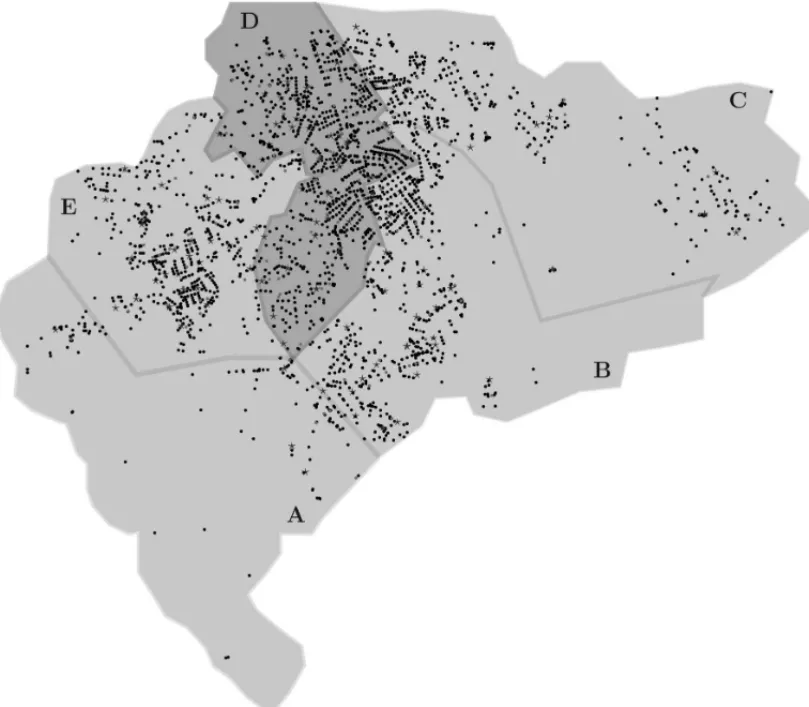
Ideally, the patrolling officers must stop in each visit point, interact with the people there, and watch certain points of interest within viewing distance. Aiming a greater proximity with the community, the chief of operations needs to designate a balanced set of visits for the patrolling cars, reducing the number of persons per officer. However, in practice, the city is divided into sectors (see Fig. 3), and a certain number of vehicles is assigned to a given sector. Moreover, the patrolling officers make the circuit of visits empirically, based on their knowledge of the geographical area, which may be unproductive. Figure 3 illustrates the distribution of five sectors within the Vinhedo city region, denoted by A, B, C, D and E. Note that the geographical points are not equally distributed within these sectors.
There are regions where the geographical points of interest are more concentrated than others, due to the characteristics of a geographical area (e.g., the distances between two schools may be much larger in peripheral areas than in central ones). Consequently, if we obtain balanced routes, there might be shorter routes in the central regions than in peripheral ones. Therefore, the fact that there are routes which are shorter than others is not inconsistent with our proposal for building routes for urban patrolling, since the efficiency of the contacts established by the patrolling officers with the members of the community outweighs the balance among the lengths of routes.
In our approach, we aim to build routes in the context urban patrolling that balance the number of visits without a prior division of the geographical area into sectors. The set of visits for each patrolling car is decided by dividing the set of all visits into clusters. Once the set of visits for a patrolling car is obtained, to determine the order to the visits, we have chosen to minimize the overall length of all routes instead of choosing the order empirically. Thus, the problem is modeled as an integer programming problem whose the main objective is to determine balanced circuits in number of visits for each patrolling car.
city of Vinhedo, the true path lengths (corresponding to routes using the city streets) were not known. Therefore, the Euclidean distance was chosen as an approximation to determine each route. Note that once the order of visits is established, the patrolling officers can use their expe-rience to decide how to go from one visit to the next.
There are similarities between the design of routes for urban patrolling and the model presented in this paper, namely, the construction of circuits covering certain geographical points, while visiting mandatory and optional ones. The number of visits is balanced and the number of routes is fixed (we do not want cars and personnel idling at the base). Throughout the text we present our model, and more importantly, our strategy to obtain approximate solutions.
The model involves a graphG=(V∪W,E), whose nodes correspond to strategic geographical points, e.g., intersections, certain locations, etc., that are either important on its own, or serve to establish reference locations for the routes. The node set is partitioned into two subsets: V = {0, . . . ,n}is the set of nodes that may belong to routes andW = {n+1, . . . ,n+ℓ}is the set of nodes that must be covered, but not visited. The setV contains a subsetT of nodes that must be visited. Node 0∈T corresponds to the base. The setV \ {0}is denoted byV∗. The symbolT∗ denotes the setT \ {0}.
The set E contains all possible undirected arcs between nodes ofV. The entryci j, of the
dis-tance matrixC =(ci j), contains the Euclidean distance between nodesi,j =0,1, . . . ,n+ℓ.
This assumption implies thatC is symmetric with zero diagonal. In this case, we choose to represent the set (undirected arc){i,j}by the ordered pair(i∗,j∗), wherei∗ = min{i,j}and j∗=max{i,j}. The size of the fleet is denoted bymand the admissible distance from a node in the route to a node that must be covered is denoted byc. We need one last parameter, to express our tolerance regarding the lack of balance between different routes. We compare routes by means of the number of nodes each route contains. The numberrdenote the maximum dif-ference allowed for the total visited nodes in any two routes.
We want to constructmroutes satisfying the following conditions:
• Each route is a circuit inGcontaining node 0.
• Each node inV∗must belong to at most one route.
• Each node inT∗must belong to exactly one route.
• There must be at least a visited node at a distance of at mostcfrom each node inW.
• The number of nodes in any two routes differ by at mostr.
urban patrol routes. In places where medical services for small villages are rendered by mobile units, their routes must be planned in such a way that, in addition to visiting specific locations, the villages not included in the tour must be within walking distance from some other village included in the tour. The model can also fit situations in business sectors, see Simms (1989) for an application in dairy practice.
The special case ofm-CTP whereV =T reduces to a vehicle routing problem (Laporte, 1992) with unit demand. Baldacci et al. (2005) present three Scatter Search heuristic algorithms for the 1-CTP. Motta et al. (2001) use a GRASP approach to solve a variant of the 1-CTP, the Gener-alized Covering Tour Problem, whose minimum length tour may pass through a subset ofW. In another point of view, Jozefowiez et al. (2004, 2007) present a multi-objective covering tour problem, a generalization of the 1-CTP where the parameterc is omitted and replaced by an objective. They propose a hybrid strategy approach that combines a multi-objective evolutionary algorithm with a branch-and-cut algorithm to determine the Optimal Pareto sets.
H`a et al. (2013) obtained exact solutions for a variation ofm-CTP, where the constraint on the length of the routes is relaxed. They used a branch-and-cut algorithm and a metaheuristic (based on the evolutionary local search) to obtain those solutions. Jozefowiez (2014) and Lopes et al. (2013) used a branch-and-price algorithm, in which a column generation approach is applied at each node of the search. Despite the recent applications form-CTP using variations of the exact methods branch-and-bound, branch-and-cut, and branch-and-price, we did not succeed in solving large instances. In our application, in the context of urban patrolling, the instances are of the order of more than two thousand points.
3 MATHEMATICAL FORMULATION OF THE PROBLEM
In order to facilitate the modeling of the covering restrictions, we define the set of nodes inV within the allowed prescribed distancecfrom each node j ∈ W: Sj = {i ∈ V |ci j ≤ c}. We
may suppose without loss of generality that|Sj| ≥2, since if there is only one nodei∈V close
enough to some j, then we may as well includei ∈ T and eliminate j fromW. Similarly, we may assume thatSj∩T = ∅, for all j, since we do not need to worry about covering nodes that
are close enough to some node inT. With these assumptions,Sj = {i ∈V\T |ci j ≤c}and its
cardinality is at least two, for all j ∈W.
The model contains two sets of binary variables. The variable yik is 1 if nodei is visited by
vehiclek, and 0 otherwise, fori ∈V,k=1, . . . ,m. The variablexi j k is 1 if vehiclekuses arc
(i, j)in its route, and 0 otherwise.
Min
m
k=1
n−1
i=0
n
j=i+1
ci jxi j k, (1)
s.t.
m
k=1
i∈Sj
m
k=1
yik≤1, i∈V \T, (3)
m
k=1
yik=1, i ∈T∗, (4)
h−1
i=0
xihk+ n
j=h+1
xh j k=2yhk, h∈V∗, k=1, . . . ,m, (5)
i∈S, j∈V\S
orj∈S,i∈V\S
xi j k≥2yhk, S⊂V∗, h∈S,
2≤ |S| ≤n−1, k=1, . . . ,m,
(6)
n
i=1
x0ik =2, k=1, . . . ,m, (7)
n
i=1
yi p− n
i=1
yiq ≤r, p,q =1, . . . ,m, (8)
n
i=1
yi p− n
i=1
yiq ≥ −r, p,q =1, . . . ,m, (9)
y0k=1, k=1, . . . ,m, (10)
yik,xi j k ∈ {0,1}, i,j ∈V, k=1, . . . ,m. (11)
Using these variables, the “cost” of a solution, given in (1), is the cumulative length of all routes, which we wish to minimize. The constraints are modelled as follows. The covering of node j ∈ W is guaranteed by (2). Constraints (3) make sure that each node inV \T belongs to at most one route. The fact that every node inT must be visited by some tour is expressed in (4). Constraints (5) imply that, if nodeh belongs to routek, then it has two neighbors in the route. Constraints (6) avoid subtours, by forcing that, if nodeh ∈ S ⊆V∗belongs to routek, then the cut-set(S,V \S)must contain at least two arcs of routek. (7) guarantees that each route has two arcs incident to the base. The maximum difference between the number of nodes of different routes is enforced by (8) and (9), i.e., the maximum difference
˜
r = max
1≤p,q≤m n
i=1
yi p− n
i=1
yiq
obtained in the solution must be less than or equal to the parameterr. Constraints (10) force that the base belongs to every route. The last set of constraints, (11), simply specifies the allowed values for the variables.
4 HEURISTICS
are selected, whereVkandWk are the nodes that may be visited and that should be covered by
routek, respectively. Phase 2 deals withm1-CTP problems, defined on the subgraph induced byVk∪Wk. At this point,mclosely related problems are considered separately. The last phase
tries to improve the solution by taking this interrelation into account. The three-phase sequence is repeated according to a criterion specific to the routine employed in Phase 1. The best solution in the whole loop of three phases (orouter iterations) is selected.
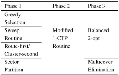
Table 1 below summarizes the routines employed in each phase of the various heuristics. The routine employed in Phase 1 will lend its name to the heuristic. Note that they share Phase 2, and the first three heuristics use Balanced 2-opt in Phase 3, while the Sector Partition uses Multicover Elimination.
Table 1–Routines according to Phase.
Phase 1 Phase 2 Phase 3
Greedy Selection
Sweep Modified Balanced
Routine 1-CTP 2-opt
Route-first/ Routine
Cluster-second
Sector Multicover
Partition Elimination
Our mathematical model resembles the model in Hachicha et al. (2000). However, in that model the length and number of visits per tour are limited and the number of routes is variable, whereas in this model the number of visits is balanced and the number of routes is fixed. In order to take into account these differences, we consider modified versions of the sweeping algorithm, Route-first/Cluster-second algorithm and 2-opt∗algorithm presented in their paper. TheSweep Routinecorresponds to steps 1 and 2 of the sweeping algorithm. Similarly, Route-first/Cluster-secondis formed by steps 1 and 2 of the algorithm of same name. TheBalanced 2-optroutine contemplates improvements via arc swapping, and is adapted from the 2-opt∗algorithm.
TheModified 1-CTP Routineis a modification of the heuristic described in Gendreau et al. (1997) for the covering tour problem. The remaining routines were developed by us.
The Greedy Selection routine gradually selects sites using a criterion that selects the nearest site to the one previously selected, forming a circular ordered list. The nodes in this list are then partitioned intomsubsets of approximately equal size, keeping the order of the original list and starting with the first node in the list. In subsequent iterations, the selection step is not repeated. Instead, we simply shift by one the order of the nodes in the list and redo the partitioning. This is repeated approximatelyt/mtimes, wheretis the cardinality of the list.
shift of the sectors. This simple geographical division is used to reduce the computational time in Phase 1.
TheMulticover Eliminationchecks whether some node inW is covered by more than one node included in a route. If this is the case, there may be room for improvement, by removing one of the superfluous nodes.
In the described routines, it is often necessary to know the subset of nodes inW covered by a particular node in V. The subset covered by node i is denoted byCi = {j ∈ W | i ∈ Sj}.
Recall thatSj = {ℓ∈V \T |cℓj ≤c}.
4.1 Greedy Selection
Initially we form a single routeR =(h0,h1, . . . ,hz)that contains all nodes inT and covers all
nodes inW as follows. The routine starts withh0 =0, R =(h0)andL =T∗∪W. The set L
is gradually emptied using the criterion that selects the nearest site to the one previously selected inL. If the chosen nodeh belongs toT, it is simply appended to R, and{h} ∪Chis removed
fromL. Ifhbelongs toW, then one selects fromShthe node that covers the greatest number of
yet uncovered nodes, say nodeℓ, and appends it toR. ThenCℓis removed fromL.
In the next two paragraphs, we detail the main differences between our approach and Hachicha’s Sweep and Route-first/Cluster-second routines. There, the selection of the setsVkandWk,k =
1, . . . ,m, is made in order to minimize the number of routes, while satisfying the demand, the capacity of the vehicle and their constraints on the length of the routes. In our approach, we chooseVkandWkwith approximately the same number of elements to keep the balance among
routes.
Here, and in the next two routines, onceRis constructed we consider the sequenceR∗ =R\ {0} as a circular list. In order to apply Phase 2, we need to divideV,T, and W intomsubsets that are induced by a partition of R∗ as follows. Let p = ⌊z/m⌋, q = z−mp, wherez denotes the number of nodes inR∗. Starting from the first node inR∗, we selectqsubsets of sequential nodes of size p+1, andm−q subsets of size p. The nodes inV (resp., T) in thekth subset union{0}are denoted byVk(resp.,Tk). Thekth subset ofW isWk={Ci |i∈Vk}.
In the next round, the partition ofR∗will start at the second node, and then third, and so on, in a total ofporp+1 outer iterations, depending on whetherzis a multiple ofmor not.
4.2 Sweep Routine
The difference between this routine and the previous one is the strategy used to build the single routeR =(h0,h1, . . . ,hz). The sweeping process is applied to the verticesT ∪W and several
solutions are generated. The routine starts withh0=0, R=(h0)andL =T∗∪W. Choose an
arbitrary nodeh¯ ∈L and consider a half line fromh0passing throughh¯. The set Lis gradually
is removed fromL. Ifhbelongs toW, then one selects fromShthe node that covers the greatest
number of yet uncovered nodes, say nodeℓ, and appends it toR. ThenCℓis removed fromL. OnceRis constructed, the process continues as in the Greedy Selection routine.
4.3 Route-first/Cluster-second
Again, the difference between this routine and Greedy Selection routine is the strategy that we build the single route R = (h0,h1, . . . ,hz). Here, a feasible 1-CTP solution for V, T,
andW is determined by means of the Modified 1-CTP Routine (section 4.5), say routeR =
(h0,h1, . . . ,hz),h0 = 0, that contains all nodes inT and covers all nodes in W. This tour is
then divided into smaller feasible routes as in the Greedy Selection routine.
4.4 Sector Partition
This routine is applicable only in cases where there is a geographical model of the problem. The site associated with the base node is taken as the geographical center of a circular disk con-taining all locations (nodes) under consideration. This disk is partitioned intomcircular sectors of same central angle. Nodes corresponding to sites in thekth partition form the setsVk,Tk, and
Wk. The first partition is arbitrary. In the next iteration, the sectors are shifted counterclockwise
by 360◦/t, and this is repeated until we return to the original partition, a total oftouter iterations. In the computer experiments, the valuet =10 was used. Due to its simplicity, if the distribution of nodes is non-uniform, this way of choosing the partitionsVk,Tk, andWkdoes not guarantee
the equilibrium among the number of nodes in each partition, possibly producing unbalanced routes.
4.5 Modified 1-CTP Routine
Gendreau et al. (1997) developed a heuristic for the covering tour problem (1-CTP), using el-ements of the GENIUS heuristic for the traveling salesman problem (TSP) of Gendreau et al. (1992) and PRIMAL1 set covering heuristic of Balas & Ho (1980).
This heuristic uses the fact that, if the set of nodes that should be visited (that is, the support of the optimal y) is known, then the covering tour problem reduces to a traveling salesman problem. This suggests the construction of a covering problem by considering the “covering” aspect separately, namely the combinatorial optimization problem (12) below. Notice that, since m=1, there is no need for the tour indexk.
Min
j∈V
cjyj ,
s.t.
j∈Si
yj ≥1, i ∈W, (12)
yj =1, j ∈T,
In PRIMAL1, variables yj are gradually included in the solution according to a greedy rule,
using one of three merit functions: (i) f(cj,bj) = cj/(log2bj); (ii) f(cj,bj) = cj/bj;
(iii) f(cj,bj)=cj; wherebjis the number of uncovered (in the current partial solution) nodes
inW that are covered by j, andcj is the cost to insert j in the current solution.
On the other hand, TSP routes are also constructed incrementally in GENIUS. During the con-struction phase, a tentative tour is built starting with three arbitrarily selected nodes and using a general insertion procedure (GENI), with rules for selecting candidates and rules for evaluating the inclusion in the tour. Once a complete tour is obtained, one seeks to improve it by removing and reinserting each node of the tour, in a post-optimization procedure called US (for Unstringing and Stringing).
GENIUS and PRIMAL1 are combined to produce a covering tour heuristic as follows. Nodes are gradually selected and added to the set of nodes that should be visited, and a new approximate solution to the TSP involving each insertion of these nodes is obtained using GENIUS. This procedure stops when all nodes inW have been covered. The selection of the each node is made by considering the merit functions in PRIMAL1 heuristic using the coefficientcj (cost to insert
this node in the approximate solution to the TSP, calculated by GENI selection rules). At the end, post-optimization is applied by removing superfluous nodes. The whole process is done for each merit function, two sequences of the merit functions (i)-(ii)-(iii) and (i)-(iii)-(ii) are considered, and the best solution is selected.
Numerical experiments with our code for the various heuristics showed that the GENI part was fast and produced acceptable results, whereas the post-optimization US routine was quite costly. After several trials, we arrived at a modified routine of Gendreau et al.’s covering tour heuristic, in order to avoid the repeated construction of unnecessary approximate solutions of the TSP at the insertion and removal of each node. This is done by inserting the new node using GENI rules and removing superfluous nodes using US rules without discarding the previous TSP solution.
More details about the experiments with the different heuristics tried out, which showed a better computational performance with these modifications, can be found in Oliveira (2008). In the modified routine listed below, the merit functions are used in the sequence (i)-(ii)-(iii).
STEP 1.Let H ←T,¯z← ∞. Let f be the merit function specified in (i). Letzbe the value of the tour obtained applying GENIUS to the TSP involving the nodes in H. If all nodes inW are covered, go to Step 2. Otherwise, go to Step 3.
STEP 2.Ifz≤ ¯z, letz¯← z,H¯ ← H. If the definition used for the merit function is the last, stop with the best solution so far, with valuez¯and set of visited nodes H¯. Otherwise, remove fromH \T nodes associated with multiple covered nodes inW using US. Go to Step 3 with the next definition of the merit function f.
STEP 3.Select withinV\Hnodeh∗using PRIMAL1, with cost coefficientscjcalculated
H∪ {h∗}. Repeat the process until all nodes inW are covered. Letzbe the value of the tour obtained. Go to Step 2.
When this routine is used in Phase 2, it is run m times with the sets Vk, Tk, and Wk, for
k=1, . . . ,m, constructed in Phase 1.
4.6 Balanced 2-opt
This is a modification of the 2-opt∗heuristic. The changes introduced aim to keep the balance, in terms of number of nodes, among the routes. Steps 1 and 2 are adaptations, since in their approach, the number of the routes can decrease and changes between arcs are allowed provided the length of the routes and number of visits are within the preset values, while in our approach, those changes can be made only if the balance between routes is not destroyed and the number of routes is not altered (we do not want cars and personnel idling at the base). Step 3 is different, it considers swapping of nodes belonging to different routes. Notice that the exchanges considered in this last step do not alter the number of nodes in each route.
At this point, the initial set ofmroutes constructed in Phase 1 has already undergone improve-ment in Phase 2, and the following procedure is executed.
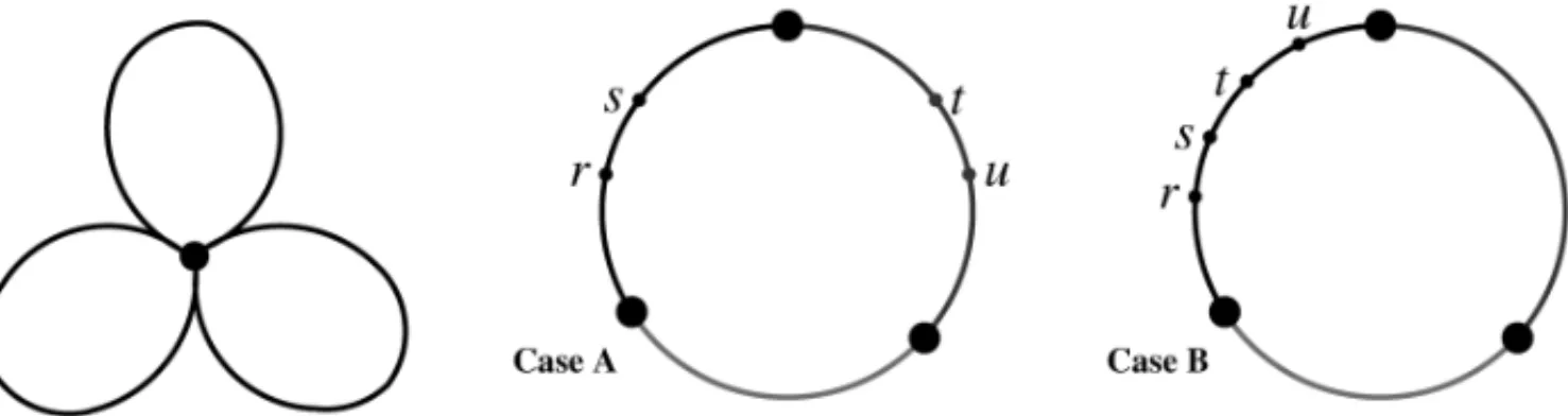
STEP 1. Let ρ be the smallest number of nodes per route, excluding the base node. Transform the set ofmroutes into a single route by replacing the base node bymartificial copies of the base node (see Fig. 1). Make a list of all possible pairs of distinct arcs in this single route.
Figure 1– How to build a single route form=3, and two patterns of arc-pairs.
must be at leastρ. For each feasible solution, calculate its objective value. If there is an improvement, recovermroutes from the best improved single (or pair of) route(s) and go back to Step 1. If the end of the list is reached without (feasible) improvement, recoverm routes from the best improved single (or pair of) route(s) and go to Step 3.
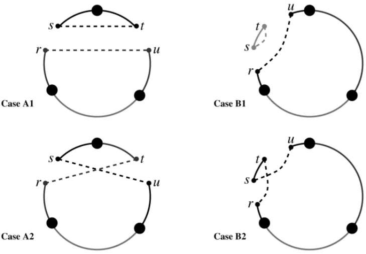
Figure 2– Two cases of replacement of arc-pairs (Cases A and B in Figure 1).
STEP 3.Make a list of pairs of nodes, each distinct from the base node, and belonging to different routes. Consider the pairs sequentially. For each pair, calculate the value of the alternative solution obtained by swapping the nodes. Keep the solution with best objective function value.
In Step 1 of the Balanced 2-opt, we transform the set ofmroutes into a single route (Fig. 1) in the same manner as described in Lenstra & Rinnooy Kan (1975). Case A and Case B in Figure 1 are two possible configurations of arc-pairs in distinct routes and in the same route, respectively. The choice ofρas the smallest number of nodes per route, and the fact that of the arc-pair exchanges in Step 2 produces routes with at leastρnodes guarantees the balance among routes.
Several patterns resulting fromk-opt moves are not suitable to our model, since they destroy the balance and create disconnected subroutes. Figure 2 (as in Hachicha et al. (2000)) illustrates some examples of configurations after the replacement of arc-pairs, where four cases are obtained according to the relative position of each arc-pair, namely the arc-pairs being either in distinct routes (Cases A1 and A2) or in the same route (Cases B1 and B2).
In Case A1, the two disconnected routes obtained are feasible once the balance constraints are satisfied. Note that this exchange is not allowed in thek-opt moves. In Case A2, one can produce unbalanced solutions depending on the number of nodes between the copy of the base and an arc-pair node. Case B1 is infeasible since one chain does not contain a copy of the base. Finally, in Case B2, there is a change in the order of nodes in a route, which may improve the solution.
4.7 Multicover Elimination
If a node inWis covered by more than one node, we may improve the solution by eliminating one of the superfluous nodes. At this point, the initial set ofmroutes constructed in Sector Partition has already undergone improvement in Phase 2. Note that only nodes inV \T (the support ofy that are not inT) may be removed from the solution. If a nodei may be removed, we consider the alternative solution obtained by deleting the arcs incident toi and adding the arc linking its neighbors. Observe that, since the distances between nodes satisfy the triangle inequality, the removal of a node always implies in the decrease of the objective function.
The possibility of removal of nodeiis checked in the brute force way: we delete it from the route and check whether this results in some node inWbeing uncovered. This is a two-step procedure. In the first step we build a list of candidates for removal, and in the second step we examine the list sequentially, trying to remove as many nodes as possible.
STEP 1.Examine all nodes in the route that belong toV\T and build a list of superfluous nodes in descending order with respect to the amount of decrease in the objective function implied by their removal.
STEP 2.Consider the nodes in the list sequentially and remove the nodes whose removal does not destroy the required coverage and balance among routes.
Note that this procedure is simpler than the Balanced 2-opt routine and it was chosen as the post-optimization for Sector Partition heuristic in order to reduce the computational time in Phase 3.
5 NUMERICAL EXPERIMENTS
The heuristics were tested on a set of adapted instances from TSPLIB and on an instance con-structed from official data of the city of Vinhedo, S˜ao Paulo. They were implemented in MAT
We close this section with statistics summarizing the test results and comments on the perfor-mances of the different heuristics.
Data Instances
The full characterization of an instance involves the following parameters: the cardinalities of the setsV,T, andW; the distanceccalculated from the setsSj, j ∈ W; the numberm; and the
parameterr(the maximum difference allowed between the number of nodes in different routes).
In order to observe the behavior of the heuristics with respect to scale, we have designed five classes of problems, where each class is defined by the total of nodes inV∪W: the first class has |V| = 50,|W| =50 corresponding to KroA100, KroB100, KroC100, KroD100 and KroE100; the second class|V| =50,|W| =100 corresponding to KroA150 and KroB150; the third class |V| = 100,|W| = 100 corresponding to KroA200 and KroB200; the fourth class|V| = 100, |W| = 218 corresponding to lin318; and the fifth class|V| =200,|W| = 200 corresponding to rd400. Each class is subdivided in three subclasses, according to the cardinality of T: the subclass 1 has|T| = ⌈|V|/8⌉; the subclass 2 has|T| = ⌈|V|/4⌉; and the last one has|T| = ⌈|V|/2⌉.
Each instance is characterized by a collection of pairs{(xi,yi)|i =1, . . . ,|V| + |W|}, where
bothxi andyi are interpreted as coordinates of points in the Euclidean plane. The base
coordi-nates are chosen from the collection so that it is centralized. Pairs corresponding to the nodes in T∗are chosen sequentially in this list, and are followed by the pairs corresponding to the nodes inV \T. All other pairs correspond to nodes inW.
Next we choose the constantcused in the definition of the neighborhoodSjof nodej ∈W. That
is, the nodes inVwhich are close enough to jin the sense that jwill be considered covered if the route contains a node inSj. The following considerations guide our choice. We want|Sj| ≥2,
for all j, socmust be greater than the maximum of the distancescj h(j), for all j ∈ W, where h(j)is the index of the node inV that is the second closest node to j. Furthermore, we want that every node inV\T covers some node inW, otherwise this node could be eliminated from consideration in a pre-processing run. Thus, we also wantcto be greater thanmh, the distance
from nodeh toW, for allh ∈ V \T. The value ofcis thus the greatest of the two maximum distances.
The number of routesmvaried from 2 to 4 in the classes with 100 and 150 points, from 3 to 5 in the classes with 200 and 318 points, and from 4 to 6 in the class with 400 points. Classes with 100 and 150 points haver =2, the classes with 200 and 318 points haver =3, and the class with 400 points hasr =4.
City of Vinhedo Instance
The geographical coordinates of the Municipal Guard base gave us the base node location. This real instance thus had 102 nodes inT, 133 nodes inWand 2496 nodes inV\T (the intersections). Figure 3 shows the distribution of points within the city region.
Figure 3– Distribution of relevant nodes in the City of Vinhedo.
Summary of Results for TSPLIB Instances
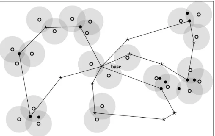
Figure 4 shows a typical solution of the problem. Notice that the three routes contain all nodes in T (the star shaped nodes), but some nodes inV \T (bullets) were not picked. The gray disks are the neighborhoods of the nodes inW (circles). One can verify that the solution is feasible with respect to coverage, as well as each gray disk contains at least one visited node. Furthermore, the routes are balanced, differing by at most one node.
Figure 4– Example of a feasible solution.
Tables 2, 3 and 4 summarize the relevant data collected in the numerical experiments with the four heuristics listed in Table 1. The first column indicates the instance, the second column the number of vehicle, and for each heuristic we report ther˜ (the maximum difference obtained between the number of nodes of different routes in the approximate solution), the time (in sec-onds) spent on each instance, the cost (total length of all tours) and the quality index (Q.I.) of the heuristic. This last number is the cost divided by the minimum cost over all four heuristics, showing how good the performance of that heuristic was, as compared to the one with the best cost. Therefore, the Q.I. of the routine with the best cost is 1, and the table cell containing this entry is shaded for emphasis.
W A S H ING T O N A LV E S DE O L IV E IRA , A NT O N IO CA RL O S M O RE T T I a n d E DNE I F E L IX RE IS
633
m r˜ time cost Q.I. r˜ time cost Q.I. r˜ time cost Q.I. r˜ time cost Q.I.
Kro-100 2 0 17.6 13465 1.377 1 7.1 10416 1.065 0 14.7 10498 1.074 0 9.4 9777 1
A 3 0 3.8 14962 1.160 2 3.2 12896 1 1 2.7 13194 1.023 0 3.0 13459 1.044
4 1 1.5 16045 1.078 1 2.5 14887 1 0 1.2 15186 1.020 1 2.8 15018 1.009
2 2 7.9 8827 1 2 3.9 8827 1 2 9.3 8827 1 0 3.0 10032 1.137
B 3 2 2.0 13176 1.197 1 2.8 11009 1 2 3.1 13183 1.197 1 1.6 12847 1.167
4 0 0.9 13526 1.027 1 1.7 13173 1 0 1.2 13610 1.033 1 1.2 13173 1
2 1 2.5 10606 1.087 1 2.6 9759 1 1 1.7 10606 1.087 1 2.1 9759 1
C 3 1 0.9 12095 1.074 2 1.4 11260 1 1 0.7 12450 1.106 0 1.0 12120 1.076
4 1 0.5 13640 1.060 2 1.2 12866 1 1 0.6 13699 1.065 1 1.1 13020 1.012
2 1 14.0 10526 1.022 1 9.6 10298 1 1 14.2 10526 1.022 1 8.1 10298 1
D 3 1 2.8 13306 1.045 2 5.0 12739 1 1 3.7 13279 1.042 0 2.4 13753 1.080
4 1 1.1 14777 1.034 1 3.2 14289 1 1 1.7 14474 1.013 1 1.8 14510 1.015
2 0 14.9 12191 1.150 0 3.8 10636 1.003 0 11.7 11534 1.088 0 5.8 10605 1
E 3 1 3.2 14510 1.051 2 2.5 13809 1 1 2.8 14504 1.050 2 2.2 14331 1.038
4 1 1.2 16392 1.061 2 1.7 15790 1.022 1 1.3 16787 1.086 2 1.8 15453 1
Kro-150 2 1 15.6 10275 1 2 10.5 10606 1.032 1 15.4 10275 1 1 11.9 11336 1.103
A 3 1 4.0 13385 1.030 2 4.3 13496 1.039 2 4.7 12992 1 1 4.6 13828 1.064
4 1 2.2 14790 1.030 2 4.5 14853 1.035 2 2.4 14357 1 1 2.9 14890 1.037
2 1 14.1 10395 1.043 1 10.1 10083 1.012 1 9.6 10083 1.012 0 4.3 9964 1
B 3 1 3.9 12967 1.114 2 5.9 11642 1.000 1 2.8 12967 1.114 1 2.8 11637 1
4 0 2.0 13769 1.063 2 3.4 13149 1.015 1 1.7 13696 1.058 1 2.4 12951 1
Kro-200 3 1 5.9 14962 1.038 2 11.5 14408 1 1 10.0 15327 1.064 1 13.2 14962 1.038
A 4 0 3.9 16646 1.002 2 15.0 16869 1.015 0 5.5 16616 1 0 9.3 17250 1.038
5 2 3.2 18212 1.030 2 8.6 17674 1 1 3.5 19738 1.117 1 8.0 18151 1.027
3 1 69.1 16648 1.041 1 95.3 15993 1 1 68.3 16016 1.001 2 66.8 16161 1.010
B 4 2 33.5 19148 1.096 2 91.9 17933 1.026 2 31.6 17933 1.026 2 28.0 17473 1
5 2 13.4 21192 1.047 2 59.1 20440 1.010 2 12.9 20827 1.029 2 20.9 20243 1
3 2 44.3 15293 1.039 2 27.6 14713 1 1 32.6 16630 1.130
lin318 4 2 23.0 19229 1.030 2 17.5 18670 1 0 17.7 19185 1.028
5 2 13.5 22009 1 2 11.2 22976 1.044 1 13.3 23390 1.063
4 3 998 8405 1.158 4 967 7256 1 1 650 7274 1.002
T H E M U LT I-VEH IC L E C O VER IN G T O U R PR O BL EM : BU IL D IN G R O U T ES F O R U R BAN P A T R O L L IN
G Kro-100 2 2 13.0 11781 1.076 2 12.7 10951 1 2 12.1 10951 1 1 9.0 11409 1.042
A 3 1 2.5 14943 1.195 2 6.8 12505 1 1 2.2 14216 1.137 1 3.0 13733 1.098 4 1 1.4 15026 1 1 5.0 15336 1.021 1 1.3 15203 1.012 1 1.5 15250 1.015
2 1 15.9 10975 1 1 33.5 11102 1.012 1 16.5 12340 1.124 1 15.0 10975 1
B 3 0 3.3 13245 1 2 3.1 13416 1.013 0 3.9 13245 1 0 5.8 13768 1.039
4 1 1.7 16358 1.029 2 1.8 16161 1.017 1 2.4 16511 1.039 1 2.8 15897 1
2 2 4.2 12982 1 2 25.5 12982 1 0 4.2 13224 1.019 2 4.1 12982 1
C 3 0 1.3 14211 1.012 1 12.0 14143 1.007 0 1.3 14043 1 0 1.4 14528 1.035 4 0 0.8 17227 1.100 2 8.5 15667 1 0 0.8 17328 1.106 0 0.8 17227 1.100
2 1 11.9 12739 1.101 1 18.3 11572 1 1 14.0 11855 1.024 1 12.8 11572 1
D 3 0 2.6 13522 1 2 2.6 13883 1.027 0 2.7 13522 1 0 3.4 13524 1.000
4 1 1.4 16552 1.075 2 8.2 15399 1 1 1.4 16033 1.041 1 2.8 15846 1.029
2 2 21.2 11700 1.093 2 15.5 11044 1.032 1 23.9 11029 1.031 1 16.8 10700 1 E 3 0 6.7 14252 1.072 2 8.3 13679 1.029 2 6.2 13296 1 0 3.4 14097 1.060
4 1 3.8 16947 1.061 2 6.3 15970 1 1 3.2 16855 1.055 1 2.7 16077 1.007 Kro-150 2 0 18.6 11413 1.030 1 14.1 11077 1 1 13.7 11077 1 1 9.1 11077 1
A 3 1 3.8 14333 1.064 2 6.8 13468 1 1 3.5 14113 1.048 1 3.2 13858 1.029 4 1 2.3 15239 1.039 2 6.2 15203 1.037 1 2.1 15166 1.034 1 2.3 14666 1
2 1 11.1 12685 1.032 2 17.5 12297 1 1 10.9 12384 1.007 1 10.3 12384 1.007 B 3 1 4.0 14170 1.003 1 5.4 14133 1 1 3.3 14843 1.050 1 3.7 14567 1.031 4 1 2.2 17697 1.125 2 6.1 15735 1 1 2.3 17186 1.092 1 2.9 15908 1.011 Kro-200 3 1 46.6 18033 1.061 3 88.9 16992 1 1 40.4 17187 1.011 1 45.0 17166 1.010 A 4 1 25.7 19745 1.026 3 103 19319 1.004 1 21.6 19246 1 1 26.3 19579 1.017 5 1 13.1 22718 1.038 3 14.1 22645 1.035 1 9.8 21888 1 1 14.9 21920 1.001
3 1 199 17489 1.024 3 166 17818 1.043 1 158 17184 1.006 0 105 17084 1 B 4 2 100 19142 1.043 3 118 18813 1.025 2 83.1 19017 1.036 1 50.8 18357 1 5 2 49.0 21647 1.018 3 43.6 21705 1.021 2 37.2 21266 1 0 23.8 21787 1.024
3 2 268 16821 1 2 202 16866 1.003 1 126 16975 1.009
lin318 4 2 126 20804 1.013 2 95.0 20810 1.013 1 114 20541 1
5 2 56.8 23984 1.011 2 39.6 23727 1 1 33.5 23996 1.011
4 2 1243 9338 1.184 3 670 7886 1 1 959 8334 1.057
W A S H ING T O N A LV E S DE O L IV E IRA , A NT O N IO CA RL O S M O RE T T I a n d E DNE I F E L IX RE IS
635
m r˜ time cost Q.I. r˜ time cost Q.I. r˜ time cost Q.I. r˜ time cost Q.I.
Kro-100 2 2 122 13062 1 2 196 13150 1.007 0 123 13216 1.012 0 123 13216 1.012
A 3 0 39.3 15966 1.079 2 146 14801 1 0 39.9 15410 1.041 0 38.6 16628 1.123
4 0 7.8 17937 1 2 11.2 17980 1.002 0 7.9 17940 1.000 0 8.3 18107 1.009
2 2 116 14052 1.114 2 127 12609 1 0 118 14075 1.116 0 117 14111 1.119
B 3 0 38.4 18619 1.113 2 35.7 17497 1.046 0 38.9 16903 1.011 0 39.7 16727 1
4 0 7.6 19165 1.023 2 6.7 18879 1.007 0 7.4 18744 1.000 0 7.8 18742 1
2 0 128 15287 1 2 134 15395 1.007 0 130 15287 1 0 130 15287 1
C 3 0 40.4 17157 1.012 2 166 16961 1 0 41.7 17034 1.004 0 40.4 17292 1.020
4 0 7.6 19577 1.001 2 8.1 19570 1.001 0 7.6 19731 1.009 0 7.9 19556 1
2 0 118 13854 1.046 2 145 13248 1 0 119 13680 1.033 0 116 13675 1.032
D 3 0 38.8 16375 1.012 1 41.2 16367 1.012 0 39.5 16178 1 0 39.4 16777 1.037
4 0 10.1 18158 1.012 2 121 18259 1.017 0 9.5 18442 1.028 0 9.3 17946 1
2 0 115 12542 1 0 102 12542 1 0 112 12542 1 0 111 12542 1
E 3 0 38.8 16837 1.030 1 36.3 16423 1.004 0 39.1 16352 1 0 38.7 16837 1.030
4 0 9.2 18229 1.038 2 70.8 17567 1 0 9.2 18086 1.030 0 9.4 17755 1.011
Kro-150 2 0 158 13881 1.005 0 171 15304 1.108 0 158 13881 1.005 0 158 13809 1
A 3 0 44.9 16366 1.090 2 68.1 15021 1 0 43.6 16481 1.097 0 43.5 15862 1.056
4 0 13.3 18795 1.028 1 15.4 18399 1.006 0 13.3 19389 1.061 0 13.5 18281 1
2 0 169 15096 1 2 191 15181 1.006 0 169 15236 1.009 0 169 15096 1
B 3 0 44.5 17211 1.015 0 75.4 16951 1 0 43.4 16951 1 0 43.8 16951 1
4 0 12.3 19582 1.018 2 18.4 19349 1.006 0 12.0 19341 1.006 0 12.6 19230 1
Kro-200 3 1 702 22610 1.166 3 980 19385 1 1 778 19513 1.007 1 751 19836 1.023
A 4 1 349 23658 1.074 3 767 22220 1.009 1 375 22019 1 1 375 22232 1.010
5 0 182 27281 1.130 3 608 24437 1.012 0 194 24415 1.011 0 188 24152 1
3 1 720 23552 1.151 3 957 20946 1.023 1 755 20471 1 1 762 20534 1.003
B 4 1 361 25711 1.186 3 761 22032 1.016 1 379 21683 1 1 379 22042 1.017
5 0 186 27893 1.155 3 553 24703 1.023 0 195 24572 1.018 0 195 24149 1
3 1 1158 17724 1.004 1 1170 17660 1 1 856 18088 1.024
lin318 4 2 688 21101 1.018 2 700 21311 1.028 1 466 20724 1
5 2 436 23740 1 2 458 24398 1.028 1 330 24083 1.014
4 1 2610 10207 1.103 1 2630 9252 1 1 2641 9321 1.007
T H E M U LT I-VEH IC L E C O VER IN G T O U R PR O BL EM : BU IL D IN G R O U T ES F O R U R BAN P A T R O L L IN
Table 5–Comparison with method of H`a et al. (2013).
H`a et al. (2013) Our method
instance |T| p m time cost instance |T| p˜ m r˜ heuristic time cost ratio
A1-1-50-50-6 1 6 2 0.8 9130 7 6 2 0 Route/Cluster 10.4 9777 1.071
A1-10-50-50-5 10 5 4 3.8 15440 KroA100 13 4 4 1 Greedy Selection 1.4 15026 0.973 A1-10-50-50-6 10 6 3 3.9 14064 13 6 3 2 Sector Partition 6.8 12505 0.889
B1-1-50-50-5 1 5 2 0.6 9723 7 5 2 0 Route/Cluster 3.0 10032 1.032
B1-1-50-50-6 1 6 2 0.6 9382 7 6 2 2 Sweep Routine 9.3 8827 0.941
B1-10-50-50-4 10 4 4 2.5 15209 KroB100 13 4 4 1 Route/Cluster 2.8 15897 1.045 B1-10-50-50-5 10 5 3 2.1 13535 13 5 3 0 Greedy Selection 3.3 13245 0.979 B1-10-50-50-8 10 8 2 2.0 10344 13 8 2 1 Greedy Selection 16 10975 1.061
C1-1-50-50-4 1 4 3 0.6 11372 7 4 3 2 1.4 11260 0.990
C1-1-50-50-5 1 5 2 0.7 9900 KroC100 7 5 2 1 Sector Partition 2.6 9759 0.986
C1-10-50-50-4 10 4 4 2.2 18212 13 4 4 2 8.5 15667 0.860
D1-1-50-50-4 1 4 3 0.9 11606 7 4 3 0 Route/Cluster 2.4 13753 1.185
D1-1-50-50-8 1 8 2 0.9 9361
KroD100 7 7 2 1 Sector Partition 9.6 10298 1.100 D1-10-50-50-5 10 5 4 3.4 18576 13 5 4 2 Sector Partition 8.2 15399 0.829 D1-10-50-50-6 10 6 3 2.9 16330 13 5 3 0 Greedy Selection 2.6 13522 0.828 A2-20-100-100-6 20 6 5 40 20966
KroA200 25 6 5 1 Sweep Routine 9.8 21888 1.044 A2-20-100-100-8 20 8 4 42 18418 25 8 4 3 Sector Partition 103 19319 1.049 B2-20-100-100-8 20 8 5 114 22156 KroB200 25 7 5 2 Sweep Routine 37 21266 0.960
For remaining instances, Sweep Routine has the biggest number of the Q.I. equals to 1, approx-imate 53% of total. Since the distribution of points in the instances with 318 and 400 points is non-uniform, the Sector Partition could not produce balanced routes in those instances. And the average value of Q.I. is 1.032, which again indicates similar performances with respect to the cost.
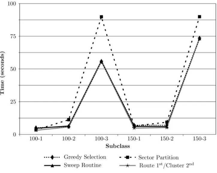
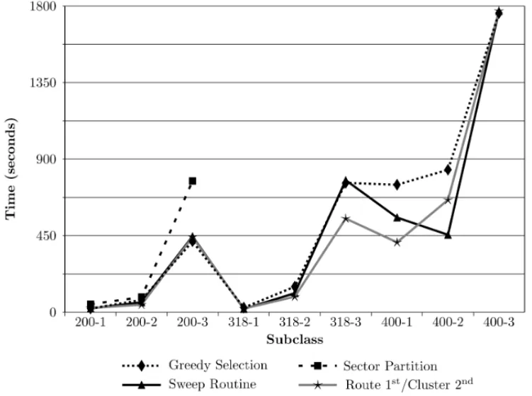
We observed discrepancies in the computational effort (measured by the average time spent) of the heuristics, as illustrated by the charts in Figures 5 and 6. The disparity of ranges led to the construction of two distinct charts. Figure 5 contains data relative to subclasses 100-1 to 150-3, the data of the remaining subclasses are in Figure 6.
Figure 5– Average times for subclasses 100-1 to 150-3.
In the first set of subclasses, the Route-first/Cluster-second is the fastest, except for the subclass 150-3, where Sweep Routine does slightly better. This pattern is maintained as the size increases, with the exception of class 400-2, where its time is 45% bigger than the minimum time.
This analysis shows that the Sector Partition is well-adapted to smaller instances, where points are uniformly distributed. For larger instances the Sweep Routine obtained solutions with better cost. In terms of speed, the Route-first/Cluster-second obtained better computation times overall, but the performances of all heuristics were very similar in this aspect.
Figure 6– Average times for subclasses 200-1 to 400-3.
formulations are that in theirs, the number of routes is not fixed, there is a constraint for the number of visits allowed on each route, and the routes may not be balanced.
In order to make a fair comparison, we consider instances in which the number of vehicles in the solution is the same in both approaches, and the maximum number of visits in our solution does not exceed their value.
The results are summarized in Table 5, which is divided into two parts, the first part contains the results from literature, namely the name of the instance, the cardinality ofT, the maximum number pof points allowed on each route, the number of vehicles, the computational time and the cost. The second part contains the our results for the same instances from TSPLIB, which satisfy the proposed conditions for the comparison. This part contains the name of the instance, |T|, the maximum number p˜of points obtained on each route,m, the value ofr˜(the maximum difference obtained between the number of nodes of different routes in the solution), the heuristic considered, time, cost, and the ratio of the cost of our heuristic to theirs.
Table 6–Results from the Vinhedo instance. Cost
Q.I. Time r r˜ Vehicles Heuristic
(Km) (sec)
106.271 1.12099 55024 6 3 5 Greedy Selection
94.801 1 50590 6 2 5 Sweep Routine
99.486 1.04942 41759 6 3 5 Route 1st/Cluster 2nd
134.857 1.42253 – 6 18 5 Empirical
114.022 1.08799 38887 8 4 6 Greedy Selection
104.800 1 36110 8 3 6 Sweep Routine
104.806 1.00006 27084 8 1 6 Route 1st/Cluster 2nd
140.735 1.34289 – 8 35 6 Empirical
121.494 1.10100 25013 8 4 7 Greedy Selection
110.349 1 23913 8 4 7 Sweep Routine
111.234 1.00802 18670 8 2 7 Route 1st/Cluster 2nd
147.700 1.33848 – 8 35 7 Empirical
is that there is no guarantee that their solutions are balanced. Finally, the proximity of the costs obtained in both formulations can be used to measure the quality of our heuristics.
Vinhedo Instance: Comparison of Heuristics
In practice, a patrolling car is assigned to a geographical area, and the patrolling officers know the locations of the visits and the points that must be observed in this area. More precisely, due to the non-uniform distribution of the geographical points, whenever the number of available patrolling cars is five, two of them are assigned to Sectors A, B and C, two cars are assigned to Sector D, and one car to Sector E. If six cars are available, one car is assigned to each of the sectors A, B, C and E, and two cars to Sector D. Finally, if seven cars are available, one car is assigned to each of the sectors A, B, C and E, and three cars to Sector D. After interviewing the patrolling officers, we noticed that given a geographical sector and set of points to be visited, the officers generally choose their routes according to a greedy rule (Empirical routes), where the next point to be visited is the nearest from the current one, which may be unproductive.
Table 6 reports the cost (in kilometers), quality index (Q.I.), time (in seconds), the value chosen for the parameterr, the valuer˜ obtained, the size of the fleet, and the heuristic considered to-gether with the empirical routes used by the patrolling officers. The numerical experimental data are collected in three cases: fleet of size five, six or seven.
Table 7–Comparative between Sweep Routine and Empirical Routes.
Sweep Routine Empirical
Cost (Km) Visits Cost (Km) Visits
Route 1 22.3154 37 29.3413 33
Route 2 22.9958 39 38.9261 47
Route 3 15.0461 37 15.9927 29
Route 4 17.3789 39 24.0204 39
Route 5 17.1356 37 26.5766 40
Average 18.9744 26.9714
Unfortunately, this did not happen in the Vinhedo instance. The geographical sites considered fit in a rectangular area of aspect ratio 1.5, that is, the width to height ratio (see Fig. 8, which shows the routes built by the Sweep Routine heuristic in the 5-vehicle case). If we were to consider the “base region” adopted for the TSPLIB instances, the base of operations should be located in a rectangle of sides 30% of the bigger rectangle, with same center. In the Vinhedo instance the base lies below and outside this ideal rectangle, missing the region by 6% of the vertical dimension.
Furthermore, the geographical distribution of sites that need to be visited or covered is highly non-uniform. If we divide the shaded rectangle of Figure 8 in four rectangles by drawing vertical and horizontal lines intersecting at the base, we will find 75.3% of all nodes concentrated in the northwest rectangle, 15.2% in the northeast, 6.8% in the southwest and only 2.7% in the southeast rectangle. As a result, the Sector Partition heuristic produced quite unbalanced routes, with the maximum difference obtained between two routes exceeding the value of the parameterr.
The speed exhibited by the Sector Partition heuristic suggests that it is worthwhile to further investigate its possibilities. One direction for future research is that of a non-uniform division in sectors, choosing the central angles in such a way that the number of nodes in each sector is approximately equal.
Compared with the artificial instances, the bad performance of the Greedy Selection heuristic was confirmed in the (very large scale) Vinhedo instance, with the highest Q.I. in every test considered. However, the Empirical routes obtained by the Vinhedo police were worse than any of the heuristics considered. Figure 7 illustrates the solution for five cars, where two cars are responsible for Sectors A, B and C, two cars are assigned to Sector D, and one car is responsible for Sector E. Considering the overall length of the routes in the first two columns of Table 6, the Empirical routes were about 33% to 42% worse than the Sweep Routine (see a example of a solution for five vehicles in Fig. 8). When compared with the Greedy Selection, the Empirical routes were about 21% to 27% worse.
Figure 7– Routes obtained empirically by patrolling officers.
Since the geographical points of interest are more concentrated in some sectors, the Empirical routes were very unbalanced, which can be seen in the fifth column of Table 6. Note that there are routes differing by 35 nodes. Moreover, in the case of five vehicles, Table 7 shows the length and number of visits for each individual route. There is a difference of up to 18 visits and the average route lengths in the Sweep Routine is about 30% lower.
The solutions obtained were considered acceptable since a patrolling car may cover this distance several times during a work shift. This contemplates very well the objective of providing a good coverage with the available resources.
6 CONCLUSIONS AND FUTURE WORK
Figure 8– Routes obtained by the Sweep Routine for the Vinhedo instance.
We developed a modified Sweep Routine, which produced solutions with lower costs for larger instances, while the Sector Partition heuristic, developed by us produced solutions with lower costs for smaller instances (up to 150 points). The computational time was quite uniform for all heuristics.
The heuristics were tested using the Vinhedo instance. The Greedy Selection heuristic, when compared with the other heuristics, produced solutions with lower quality. The solutions of our modifications of the Sweep Routine and Route-first/Cluster-second Routine had similar quality, though the former was always better. On the other hand, the latter was consistently faster.
We observed that the Sector Partition heuristic needs improvement in order to be applied in real instances having highly non-uniform distribution of nodes, turning it into a competitive and robust routine. This will be the subject of future research.
ACKNOWLEDGMENTS
The first author was partially support by CAPES and FAEPEX (grant 534/09). The second author was partially supported by CNPq-PRONEX Optimization and FAPESP (grant 2006/53768-0). The authors thank Osmir Cruz, Commander of the Municipal Guard of Vinhedo, the municipal government of Vinhedo and the company SSR-Tecnologia for translating the list of addresses into a list of geographical coordinates.
REFERENCES
[1] BALASE & HOA. 1980. Set covering algorithms using cutting planes, heuristics, and subgradient optimization: A computational study, in PADBERGM., (Ed.), ‘Combinatorial Optimization’, Vol. 12 ofMathematical Programming Studies, Springer Berlin Heidelberg, pp. 37–60.
[2] BALDACCIR, BOSCHETTIM, MANIEZZOV & ZAMBONIM. 2005. Scatter search methods for the covering tour problem, in SHARDAR, VOSSS, REGOC & ALIDAEEB., (Eds.), ‘Metaheuristic Op-timization via Memory and Evolution’, Vol. 30 ofOperations Research/Computer Science Interfaces Series, Springer US, pp. 59–91.
[3] BROWNM & FINTORL. 1995. US screening mammography services with mobile units: results from the national survey of mammography facilities.Radiology,195(2): 529–532.
[4] FOORDF. 1995. Gambia: evaluation of the mobile health care service in West Kiang district.World health statistics quarterly. Rapport trimestriel de statistiques sanitaires mondiales,48(1): 18–22. [5] GENDREAUM, HERTZA & LAPORTEG. 1992. New insertion and postoptimization procedures for
the traveling salesman problem.Operations Research,40(6): 1086–1094.
[6] GENDREAUM, LAPORTEG & SEMETF. 1997. The covering tour problem.Operations Research, 45(4): 568–576.
[7] H `AMH, BOSTELN, LANGEVINA & ROUSSEAULM. 2013. An exact algorithm and a metaheuris-tic for the multi-vehicle covering tour problem with a constraint on the number of vermetaheuris-tices.European Journal of Operational Research,226(2): 211–220.
[8] HACHICHAM, HODGSONMJ, LAPORTEG & SEMET F. 2000. Heuristics for the multi-vehicle covering tour problem.Computers & Operations Research,27(1): 29–42.
[9] HELSGAUNK. 2009. General k-opt submoves for the Lin–Kernighan TSP heuristic.Mathematical Programming Computation,1(2-3): 119–163.
[10] HODGSONMJ, LAPORTEG & SEMETF. 1998. A covering tour model for planning mobile health care facilities in Suhum District, Ghama.Journal of Regional Science,38(4): 621–638.
[12] JOZEFOWIEZN, SEMETF & TALBIE. 2004. A multi-objective evolutionary algorithm for the cover-ing tour problem.Applications of multi-objective evolutionary algorithms, COELLOCA & LAMONT GB, (Eds.),World Scientific, pp. 247–267.
[13] JOZEFOWIEZN, SEMETF & TALBIE. 2007. The bi-objective covering tour problem.Computers & Operations Research,34(7): 1929–1942.
[14] LABBE´M & LAPORTEG. 1986. Maximizing user convenience and postal service efficiency in post box location.Belgian Journal of Operations Research Statistics and Computer Science,26: 21–35. [15] LAPORTEG. 1992. The vehicle routing problem: An overview of exact and approximate algorithms.
European Journal of Operational Research,59(3): 345–358.
[16] LENSTRAJK & RINNOOYKANAHG. 1975. Some simple applications of the travelling salesman problem.Operational Research Quarterly,26(4): 717–733.
[17] LIN S & KERNIGHAN BW. 1973. An effective heuristic algorithm for the traveling-salesman problem.Operations Research,21(2): 498–516.
[18] LOPESR, SOUZAVAA & CUNHAAS. 2013. A Branch-and-price Algorithm for the Multi-Vehicle Covering Tour Problem.Electronic Notes in Discrete Mathematics,44: 61–66.
[19] MOTTA L, OCHI L & MARTINHONC. 2001. Grasp metaheuristics for the generalized covering tour problem, in ‘Proceedings of IV metaheuristic international conference, Porto, Portugal’, Vol. 1, Citeseer, pp. 387–93.
[20] NEV/USP. 2009.Manual de policiamento comunit´ario: pol´ıcia e comunidade na construc¸˜ao da seguranc¸a, Bras´ılia: N´ucleo de Estudos da Violˆencia da Universidade de S˜ao Paulo; SEDH, S˜ao Paulo.
[21] OLIVEIRAWA. 2008. Construc¸˜ao de rotas para patrulhamento urbano preventivo, Master’s Thesis, Institute of Mathematics, Statistics and Scientific Computing, Department of Applied Mathematics, State University of Campinas, Campinas, Brazil.
[22] OPPONGJR & HODGSONMJ. 1994. Spatial accessibility to health care facilities in Suhum District, Ghana.The Professional Geographer,46(2), 199–209.
[23] SIMMSJC. 1989. Fixed and mobile facilities in dairy practice.The Veterinary Clinics of North Amer-ica – Food Animal Practice,5(3): 591–601.