ISSN 0104-6632 Printed in Brazil www.abeq.org.br/bjche
Vol. 22, No. 03, pp. 419 - 432, July - September, 2005
Brazilian Journal
of Chemical
Engineering
SIMULTANEOUS INFLUENCE OF GAS MIXTURE
COMPOSITION AND PROCESS TEMPERATURE
ON Fe
2
O
3
→
FeO REDUCTION KINETICS - NEURAL
NETWORK MODELING
K. Piotrowski
1,2, T. Wiltowski
1,3,*, K. Mondal
3, L. Stonawski
1,3,
T. Szymanski
3and D. Dasgupta
31
Southern Illinois University Carbondale, Coal Research Center, Carbondale, IL 62901, USA.
2
Department of Chemical & Process Engineering, Silesian University of Technology, Gliwice, Poland.
3
Department of Mechanical Engineering and Energy Processes, Southern Illinois University Carbondale, Phone/Fax: (01) 618–453–7346,
Carbondale, IL 62901, USA E-mail: [email protected]
(Received: September 27, 2004 ; Accepted: December 17, 2004)
Abstract - The kinetics of Fe2O3→FeO reaction was investigated. The thermogravimetric (TGA) data
covered the reduction of hematite both by pure species (nitrogen diluted CO or H2) and by their mixture. The
conventional analysis has indicated that initially the reduction of hematite is a complex, surface controlled process, however once a thin layer of lower oxidation state iron oxides (magnetite, wüstite) is formed on the surface, it changes to diffusion control. Artificial Neural Network (ANN) has proved to be a convenient tool for modeling of this complex, heterogeneous reaction runs within the both (kinetic and diffusion) regions, correctly considering influence of temperature and gas composition effects and their complex interactions. ANN’s model shows the capability to mimic some extreme (minimum) of the reaction rate within the determined temperature window, while the Arrhenius dependency is of limited use.
Keywords: Artificial Neural Network (ANN); Feed–forward multilayer perceptron; Iron oxides reduction; Isothermal solid–state reaction kinetics; Topochemical reactions.
INTRODUCTION
Iron Oxide Reduction Process
The reduction of hematite (Fe2O3) to wüstite (FeO) via magnetite (Fe3O4) is regarded as a complex gas–solid topochemical reaction. It involves complex micro–structural (crystal network) changes in the intermediate oxides (Fe3O4, FeO). Additionally, in the advanced stages of the process the access of reducing gas is primarily controlled by
equation which would be valid both in the surface and diffusion controlled ranges has been formulated till the present day [e.g., Hayes (1979), Kang et al. (1996), Tokuda et al. (1973)]. Some studies [e.g., Hayes (1979), El–Rahaiby and Rao (1979), Doherty et al. (1985)] were devoted only the theoretical reduction mechanism (chemical reaction control). Generally it have been concluded, that it is a complex system of topochemical transformations whose individual rates are influenced both by chemical kinetic factors and mass (and/or heat) transfer factors. Although all these mechanisms have been established and it seems to be the agreement concerning the rate controlling reactions, the dynamic behavior of this complex, heterogeneous system is still not well elaborated. It would explain the reported no consistency in the published kinetic data.
Considering the outlined complex nature of the iron oxides transformations, taking into account the interrelated processes running in micro– and macro– scale, the mathematical description of this process is still not well advanced. One of the efficient tools, which enable one to obtain a numerical description of this kind of complex process kinetics, are the Artificial Neural Networks, which are thereby applied to this approach.
Artificial Neural Network (ANN) is regarded as
an efficient, calculation tool, since its application for practical engineering calculations does not require the initial elaboration of a physical model of the process with possible all detailed connections between the factors affecting the reaction’s run. This method enables one to obtain quickly a sufficiently precise numerical description of the process, especially if its mechanism is not completely explained or a lack of specific data precludes the elaboration of semi–empirical model. In such cases, based on (the most frequent) the experimental data the Networks are “trained” by an appropriate algorithm to numerically solve the problem and find the appropriate input–output relationships. This enables one to numerically forecast the results, being the “simulated object’s responses”, for assumed, interesting input data–sets from the examined experimental range [e.g., Stephanopoulos and Han, (1996), Willis et al. (1992)]. In the recent days the ANN has proved their usefulness within many different chemical engineering problems proved difficult for conventional modeling approaches, both applied independently [e.g., Meert and Rijckaert (1998), Hoskins and Himmelblau (1988) ] or being an integral part of the complex hybrid models [e.g., Psichiogos and Ungar (1992), Thompson and Kramer (1994)].
Figure:1 Artificial Neural Network’s scheme (multilayer perceptron–type network).
The most often used ANN’s configuration is presented in Fig.1. The input units (denoted as INPUT 1…N) are connected with “computational cells” called “neurons”, usually arranged in layers (both hidden layer – NEURONS 1… K and output layer – NEURONS O1… OL). The “power” of the adjacent neurons’ interaction is quantified by the “weight” value – an attributed numerical value,
the previous (here – first) layer’s N neurons (INPUTp) and some constant value (bi) – called “bias” (Eq.1):
N
iSUM ip p i
p 1
y w INPUT b
=
=
∑
⋅ + (1)and then transforming the result of Eq.1 (yi SUM) by adequate (the most often sigmoidal–type) transfer function (Eq. 2) to obtain its output value (yi):
(
)
iSUMN
ip p i p 1
i iSUM y
w INPUT b
1 y f y
1 e
1
1 e =
−
−∑ ⋅ +
= = =
+
=
+
(2)
The regular, stratified structure of the Neural Network enables one to perform the next consecutive transformation of the signals through the following layers in the identical manner (Eq.3), see also Fig.1:
K K N
Oi Oip p Oi Oip ip p i Oi
p 1 p 1 p 1
p
y f w y b f w f w INPUT b b
= = =
= ⋅ + = ⋅ ⋅ + +
∑
∑
∑
(3)
and then transmit it further – to all neurons of the next layer, what makes it possible to render of practically any nonlinear transformation [Hoskins and Himmelblau (1988)]. The finally transformed by “output layer” neurons (NEURONS O1…OK) the signals are presented as OUTPUT VALUES 1…M and can be delivered directly to the user. The correct data processing within the ANN structure is possible owing to the matrix of appropriate weight values. Thus, in order to prepare the ANN to “solve” a required task, there is necessity of adjusting the weight values within the wholly network first. This gradual fitting is carried into effect by learning the ANN by means of an adequate algorithm. The training is performed with the use of learning “input– output” (the most often – experimental) data sets. During the learning procedure the program iteratively compares the current values (forecasted by ANN) with the expected (experimental) ones (it is when supervised learning mode applied). Thus, adjusting step by step the entire network weights’ values (based on the actual error’s value information) it simultaneously strives to attain the best, declared compatibility between the two data sets (backpropagation error algorithm method). After the learning procedure has been finished the matrix of optimum weight’s values is prepared – accumulating hidden, complex information about the process under investigation, thus immediately ready for the practical problems solving.
The successful trials of the ANN application in chemical and process engineering problems [e.g., Piotrowski, K. et al. (2003), Galván et al. (1996), Abilov and Zeybek (2000)] have shown that simple ANNs are capable of complex nonlinear systems
modeling, the properly selected and trained Network enables one to interpolate and, in restricted range, extrapolate the data and confirmed that the Networks enable one to perform the complex design calculations quickly and effectively.
representative kinetic model for considered case because of the complexity of the reactions involved. A hybrid modeling approach was proposed for the identification of the dynamic behavior of chemical reactors [Porru et al. (2000)] to overcome this limitation. The possibility of ANN has been exploited to adequately represent the complex kinetic reaction data. The “neural reaction rate model” was integrated with a first principles model for a heterogeneous gas–solid reactor where the catalytic oxidation of CO takes place. The results confirmed that ANN can be effectively used to formulate lumped reaction rates because of their capability in capturing the essential dynamic characteristics of the functional relationship among the state variables. Other researchers [Baratti and Servida (2000)] explored the similar procedure for the case of catalytic oxidation of CO over Pt–Al catalyst. Coal, both chemically complex and heterogeneous structured species, has proved to be very difficult to construct generalized physical descriptions of pulverized combustion for incorporation into reliable mathematical models (including: pyrolysis, char devolatilization, particle/turbulence interaction, etc.) suited to industrial applications. An approach based on ANN was proposed [Abbas et al. (2003)]. It proved to be capable of handling a range of solid fuels (coal, biomass, mixtures). The ANN model was implemented into an existing 3D CFD combustion code. Its devolatilization predictions have also been compared with a detailed devolatilization model (FLASHCHAIN) and were found to be consistent. Palau [Palau et al. (1996, 1999)] focused on using ANN model to control a gas/solid sorption chilling machine. In such systems, the cold production changes cyclically with the time due to the batchwise operation of the gas/solid reactors. The accurate simulation of the dynamic performance of the chilling machine has proven to be difficult when using the deterministic models because some model’s parameters dynamically change with the reaction advancement. The ANN model has proved to be a good and fast tool for predicting the mean cooling power given by a chilling machine under different operating conditions. Since it is necessary to predict sintering quality in order to realize optimization of technology parameters in sintering process, ANN was successfully used to build up a prediction model for FeO content during the sintering process [Zhang et al. (2002)].
The aim of the presented work was to test the ANN capabilities for modeling of the kinetics of a complex heterogeneous process of iron oxides reduction, especially to test the simultaneous
influence of temperature and reducing potential of various reactants. Considering the accessible literature data, excluding the authors’ own elaboration [Wiltowski, T. et al. (2004 a,b)] there is no reported literature of any ANN application devoted to this complex and industrially important process. Particularly, the Fe2O3 – FeO conversion degree (α) courses, which depend on the process temperature, time and reducing mixture’s chemical composition as well as of their unpredictable complex interactions, were elaborated.
EXPERIMENTAL SECTION
The experiments were performed using the Perkin–Elmer TGA–7 thermogravimetric analyzer driven by Pyris software. Samples of Fe2O3 powders (PEA Ridge Iron Ore, Co.) were preheated (100C/min) under the inert N2 atmosphere to the desired temperature (700–9000C). The reducing gases were then introduced under isothermal conditions and flow rate of 30 ml/min. The gases were dried before their use in molecular sieve moisture trap Hydro–Purge II, Alltech. The initial weight of Fe2O3 samples in all cases was approx. 12 mg. The kinetics of hematite–magnetite–wüstite reduction was determined by monitoring the weight change experienced by the specimen during the course of its reduction under isothermal conditions. The overall process course for iron oxides reduction is stoichiometrically as follows:
Fe2O3 ? Fe3O4 ? FeO (4)
Since Fe3O4 can be viewed as a mixture of Fe2O3 and FeO, the theoretical specimen weight decrease can be calculated from the following reactions (stoichiometry):
Fe2O3 + CO? 2FeO + CO2 (5)
Fe2O3 + H2 ? 2FeO + H2O (6)
change (m0 - m10%). The experimental data were then converted into the α(0 – 1) range using the following formula:
( )
00 10%
m m(t) t
m m
−
α =
− (7)
The experimental α = f (t) runs (Eq. 7) obtained within the temperature range studied (700–900oC)
are presented in Fig. 2 [Piotrowski, K. et al. (2004 a,b)]. The α = f (t) time – plots are visible sigmoid shaped and exhibit three distinct ranges: incubation, acceleratory and decaying periods [e.g. Tokuda et al. (1973)]. An increase in temperature results in a shorter incubation period while the kinetic rate of reduction is observed to be considerably accelerated. However, the general shape of the curves within the temperatures of interest is observed to be similar (for each mixture composition separately – see Fig. 2).
(a) (b)
(c)
NEURAL NETWORK CALCULATIONS
Training and Validating of ANN
The experimental TGA raw data, preprocessed using Eq.(7), were the basis for the process of the ANN preparing – learning and testing. The 644 input–output data sets consisted of coupled input (process temperature (T), time (t), hydrogen content (vol %) in the reducing gas – considering the constant 90% N2 it was informative enough considering the gas composition) and corresponding output (Fe2O3 – FeO conversion degree, α) data. The experimental data covered the temperature range of 700–910oC, process time of 0 – 5 min and 0 – 10 vol. % of H2 (corresponded to 10 – 0 vol.% of CO while assumed 90 vol.% of N2 as constant). A feed– forward, multilayer ANNs with three inputs (T, t and [H2]), one output neuron (α) and of diversified combination of the hidden layer’s dimension and structure were used for the numerical simulation of the process. The 535 randomly selected sets of the data (T, t, [H2] - α) were used for the ANN learning (learning data), since the other 109 sets (testing data) of identical structure were applied to verify simultaneously the correctness of the current responses providing by the ANN. This procedure protected the ANN structure against the overtraining effect (fitting exclusively to the learning data without any generalization capabilities) thus making the determination of optimal iterations number permitted for each learning run. The all assumed ANN’s structures were implemented and simulated with the use of DynaMind software. Neurons of sigmoidal type (Eq. 2) were used with a continuous activation function whose output values changed from 0 to 1. Before the learning process started, the input–output data sets’ raw numerical data (T, t, [H2]) had been scaled into 0–1 window to fit within the transfer function, Eq. (2), limits.
The learning procedure (supervised learning) was executed for a selected number of “test” configurations (Tab. 1) taking advantage of the backpropagation error algorithm, employing gradient – descent strategy of error function minimalization. The learning process was terminated at the moment of beginning of the test set error’s increase. This way it corresponded to the optimum value of the weights’ matrix.
After the learning procedure has finished the comparative analysis of the agreement between the raw experimental data and ANN’s calculation results was carried out. The all 644 data sets were
considered each time for every net’s configuration (40 structures – see Tab. 1) verified. For intermediate tests purposes (comparing the n ANN’s results (αcalc
) with the n experimental ones (αexp)) the following statistical indicators were applied:
Mean Deviation (MD)
(
calc exp)
MD
n
α − α
=
∑
(8)and Root-Mean Square Deviation (RMSD)
(
calc exp)
2 RMSDn
α − α
=
∑
(9)The data in Table 1 indicates that the optimal configuration of the ANN, denoted as notation of (3– 20–1), corresponded to 20 neurons in one hidden layer (3 inputs and 1 output comply with the learning and testing data–set structure). The optimum iterations’ number (assuming the learning rate parameter’s optimal value of 0.1, avoiding falling into the local minima without the momentum element application) was 3200 (optimized for the sake of overtraining effect). The ANN’s learning process was performed several times starting with different, randomly selected matrices of initial weight values. As the results, the set of ANN of similar exactness was obtained. On the basis of the optimal configured and trained ANN, (3–20–1), the dependencies of Fe2O3 → FeO conversion degree (α) on the process parameters (t and [H2]) assuming gradually elevated temperature T values were modeled, testing the reducing potential of various compositions (kinetic behavior) for selected thermal conditions.
Reduction Process Modeling
Table 1: Artificial Neural Network configurations tested – agreement between the Neural Network answers and experimental data
#
Network configuration (inputs – hidden neurons – outputs)
Optimum iterations number
α MD
α RMSD
One hidden layer
1 3 – 2 – 1 1000 0.017493 0.107971
2 3 – 4 – 1 2000 0.002058 0.039699
3 3 – 6 – 1 2200 -0.002160 0.047158
4 3 – 8 – 1 2200 -0.000760 0.036997
5 3 – 10 – 1 2200 -0.006120 0.038841
6 3 – 12 – 1 2000 -0.006760 0.048874
7 3 – 14 – 1 2200 -0.001000 0.044316
8 3 – 16 – 1 3000 0.000944 0.035105
9 3 – 18 – 1 2400 -0.001940 0.039073
10 3 – 20 – 1 3200 0.002984 0.034716
Two hidden layers – configuration 1
11 3 – 6 – 2 – 1 1200 -0.004550 0.038898
12 3 – 6 – 4 – 1 1400 -0.000400 0.044676
13 3 – 6 – 6 – 1 1500 -0.007880 0.042696
14 3 – 6 – 8 – 1 1300 0.013257 0.049524
15 3 – 6 – 10 – 1 1100 -0.003740 0.040673
16 3 – 6 – 12 – 1 1400 0.001778 0.038326
17 3 – 6 – 14 – 1 1200 -0.004910 0.041808
18 3 – 6 – 16 – 1 2200 0.007487 0.041177
19 3 – 6 – 18 – 1 1300 -0.004240 0.040041
20 3 – 6 – 20 – 1 1200 0.005916 0.039625
Two hidden layers – configuration 2
21 3 – 12 – 2 – 1 1700 -0.010660 0.054824
22 3 – 12 – 4 – 1 2300 -0.005560 0.044620
23 3 – 12 – 6 – 1 1800 0.002073 0.037207
24 3 – 12 – 8 – 1 1500 -0.009160 0.043418
25 3 – 12 – 10 – 1 1500 -0.003290 0.041404
26 3 – 12 – 12 – 1 1800 0.000200 0.039346
27 3 – 12 – 14 – 1 1900 0.004288 0.042500
28 3 – 12 – 16 – 1 1400 0.001605 0.040368
29 3 – 12 – 18 – 1 1600 -0.010650 0.041901
30 3 – 12 – 20 – 1 1500 0.008149 0.044211
Three hidden layers
31 3 – 10 – 10 – 2 – 1 1600 -0.003930 0.037405
32 3 – 10 – 10 – 4 – 1 1700 -0.005860 0.039475
33 3 – 10 – 10 – 6 – 1 1400 -0.000830 0.043896
34 3 – 10 – 10 – 8 – 1 1400 0.004633 0.041222
35 3 – 10 – 10 – 10 – 1 1800 -0.003200 0.039536
36 3 – 10 – 10 – 12 – 1 1600 0.008234 0.041262
37 3 – 10 – 10 – 14 – 1 1300 -0.013140 0.038437
38 3 – 10 – 10 – 16 – 1 1700 -0.003450 0.041561
39 3 – 10 – 10 – 18 – 1 1800 0.000464 0.038021
Figure 3: The a = f(t) kinetic profiles of iron oxide reduction process– comparison of ANN’s predictions and experimental data for the selected three process temperatures
(reducing gas of composition: 90% N2, 5% H2, 5% CO).
0 2
4 6
8 10 0.0
0.2 0.4 0.6 0.8 1.0
0 1
2 3
4 5
α
time [min]
H2 [%]
(a)
0 2
4 6
8 10 0.0
0.2 0.4 0.6 0.8 1.0
0 1
2 3
4 5
α
time [min]
H
2 [%]
(b)
0 2
4 6
8 10 0.0
0.2 0.4 0.6 0.8 1.0
0 1
2 3
4 5
α
time [min]
H
2 [%] (c)
0 2
4 6
8 10 0.0
0.2 0.4 0.6 0.8 1.0
0 1
2 3
4 5
α
time [min]
H
0 2 4 6 8 10 0.0 0.2 0.4 0.6 0.8 1.0 0 1 2 3 4 5 α
time [min]
H
2 [%] (e) 0 2 4 6 8 10 0.0 0.2 0.4 0.6 0.8 1.0 0 1 2 3 4 5 α time [min] H
2 [%] (f)
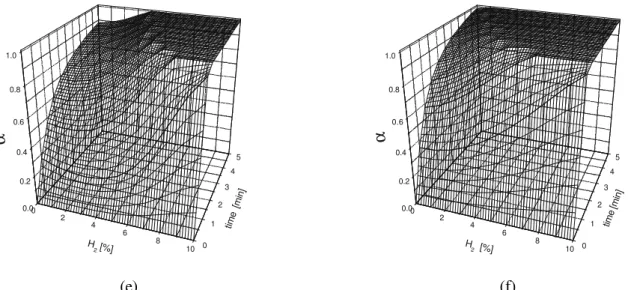
Figure 4: Iron oxide reduction process kinetics – influence of H2 content in reducing mixture in the arising process temperatures (a – 7000C, b – 7600C, c – 8200C, d – 8400C, e – 8600C, f – 9000C).
0.00 0.20 0.40 0.60 0.80 1.00
ANN predictions 0.00 0.20 0.40 0.60 0.80 1.00 E x p e ri m e n ta l d a ta (a)
0.00 0.20 0.40 0.60 0.80 1.00
ANN predictions 0.00 0.20 0.40 0.60 0.80 1.00 E x p e ri m e n ta l d a ta (b)
0.00 0.20 0.40 0.60 0.80 1.00
ANN predictions 0.00 0.20 0.40 0.60 0.80 1.00 E x p e ri m e n ta l d a ta (c)
0.00 0.20 0.40 0.60 0.80 1.00
0.00 0.20 0.40 0.60 0.80 1.00
ANN predictions
0.00 0.20 0.40 0.60 0.80 1.00
E
x
p
e
ri
m
e
n
ta
l
d
a
ta
(e)
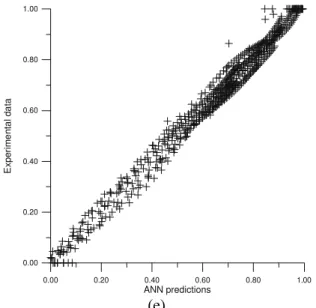
Figure 5: The comparison of “experimental vs. predicted” values of α (diagonal error plots) for the five selected ANN’s configurations: (a) – 3-8-1, RMSD = 0.036997, (b) – 3-16-1, RMSD = 0.035105, (c) – 3-20-1, RMSD =
0.034716, (d) – 3-12-6-1, RMSD = 0.037207, (e) – 3-10-10-2-1, RMSD = 0.037405.
DISCUSSION
The obtained ANN model was verified with the experimental data first. The Network’s precision is confirmed on the experimental – modeled comparative chart (Fig. 3 and 5). Considering these results, the performance of detailed analysis of the process’ behavior in various T conditions based on the ANN’s simulation results seems justified. The ANN’s numerical modeling results, presented in convenient, graphical form in Fig. 4, are discussed below.
Generally it can be stated, that both with temperature, T, and hydrogen concentration, [H2] increase, the kinetic profiles of the α (t)[H2]=const form have gradually more and more sharp courses between 0 and 1 (corresponded to full Fe2O3 to FeO conversion) values, however the hydrogen content in reducing gas seems to impose considerably stronger influence on this shape (especially in the 3 – 6 % [H2] range). With the temperature increasing, the difference in the process courses for various [H2] values is less and less clear (compare the data corresponding to 700 and 9000C). The characteristic “hill’s slope”, distinctly visible within 700–7600C window, becomes more and more unclear (820– 8600C) and practically disappears in the vicinity of temperature 9000C. Considering the diffusion range it is visible that for 10% CO case the temperature influence is of great importance for overall kinetics of the process – with the T increasing the diffusion rate increases thus the higher Fe2O3 – FeO
range it becomes possible to obtain higher conversion degrees for the same temperature. For [H2] =10% a full conversion degree is reached in a relatively short process time (less than 1 min) within the all temperatures studied. For both [H2] content and temperature increasing, the “full conversion area “ (corresponded to α = 1) constant surface is more and more widespread (compare the flat plateau indicating full Fe2O3 to FeO conversion range presented in Fig. 4). In the authors’ previous study [Piotrowski, K. et al. (2004 a,b), Wiltowski, T. et al. (2004 a, b)] it was evaluated, that activation energy value decreases considerably with the H2 content in the reducing mixture extending. The reducing mixture composed of N2 and CO only shows higher activation energy (∆Ea= 104 kJ/mol) than that for the N2 and H2 mixture alone (∆Ea= 23.85 kJ/mol). The reactions with only CO+N2 containing reducing mixture (0% of H2 corresponds in this study to 10% of CO), as characterized by higher activation energy, are very temperature sensitive [Levenspiel, O. (1988)], whereas reactions involving only H2+N2 (thus 10% H2 corresponded to 0% CO), marked by lower activation energy, are relatively temperature– insensitive (see the sharp, practically the same kinetic profile, Fig. 2). This sensitiveness is clearly observed by examining the data in Fig 4 as well, especially comparing the time–dependence for boundary profiles (cross sections of effective surface) for [H2] =0% (corresponded to [CO] =10% case) and [H2] =10% (which, in turn, seem practically invariant). Similar increases in reaction rate when hydrogen is added to carbon monoxide have been found by others researchers [e.g. Nikanorova, L.P. and Antonova, V.M. (1991), Tokuda et al. (1973)], who have attributed them to higher hydrogen’s chemical potential of reduction, as well as the higher diffusivity of hydrogen within the pores of the solid (thus mass transfer facility and better chemical properties of H2 for reduction processes). Thus, the ANN simulation results correctly reflect the increased reducing capacity of the inlet gas at higher temperatures and with enhanced of the H2 content. Increasing the proportion of CO/H2 in the inlet gas slows the reduction rate. On the other hand, the rate of reduction by CO is markedly enhanced by the H2 addition. Considering the ANN model’s features it should be mentioned, that the properly trained and validated ANN incorporates all “hidden” information influencing the process course. Thus, all side–effects and sub–processes are taken under consideration even without our knowledge about their existence. It becomes important in the complex process
description, like in considered kinetic case. After a specific period of time (depending on process conditions) the reaction shifts from kinetic range to the diffusion range. ANN model, on the other hand, was found to be useful both in kinetic and diffusion regions, incorporating all possible “intermediate range effects” acting within the shift range between the two clearly defined kinetic mechanisms. It should be pointed that mass transfer limitations, as well as the solid state transition effects must also be taken into account in a full process kinetics analysis. The endothermic nature of the process can play a significant role in the heat transfer effects, inhibiting or catalyzing the phase transformations, thus raise doubts as far as concerned the isothermal assumptions of the process conditions (usually applied in the classical approach for the difference equations’ calculations simplifying). The heat transfer can affect the surface structure’s composition and morphology, what is a key factor in diffusion processes and surface adsorption (being the first stage of many solid–state transformations). All these factors strongly affect each other, sometimes in not fully predictable manner, so the trials to create one coherent model and predict the process behavior based on kinetic information evaluated in various, considerable diversified and idealized laboratory conditions usually fail. Thus, the application of ANN for the numerical modeling of this complex process seems to be motivated and purposeful for engineering and design purposes, becoming a valuable tool for the rational optimizing of this process within the full 700 – 9000C temperature range. As a consequence of this approach one can rationally select the optimal values of the decisive process parameters, thus carry into effect the professional assessment of the process conditions. The Network’s correct prediction in the ranges where it was not provided with the training data proves its good interpolation capabilities. Hence, the Network may be applied to equalize numerically raw experimental data when it is necessary for calculation–design needs. Taking into account the difficulties and inaccuracies associated with TGA measurements, the accuracy of the results generated by the ANN can be considered satisfactory for engineering calculations. The accuracy of the results obtained from the ANN model is closely related to the accuracy and range of experimental data used for the Network learning and testing. A Network type, configuration and number of learning iterations are of great importance, too.
changes as small as 0.1 µg (thus 1 x 10⁻⁷ g). Since the initial mass of the sample was about 12 mg – its decrease by 10% corresponded to appropriately ∆m = 1.2 mg = 1.2 x 10⁻³g. This ∆m corresponded, however, to a full conversion degree (α) range (0–1). This way the accuracy of the TGA analysis in the directly relation to the conversion degree (α) can be estimated with the following simply proportion:
( )
7
5 3
1 10
8.33 10
1 0 1.2 10
−
− −
∆α = × ∆α = ×
− ×
while the statistical error indicators for the selected optimal configuration (3–20–1) based on the predicted conversion degree ( α ) deviations from the experimental ones, are as follows: MD (α) = 2.984 x 10⁻³, RMSD (α) = 3.4716 x 10⁻².
While comparing these error values one should keep in mind, that the Neural Network model’s results were computed for a wide range of all possible reaction conditions with one coherent, numerical model, capable of predicting the results of interaction of many complex phenomena. Thus, the error values (MD, RMSD) can simply result from the regression and rendering flexibilities of possibly, the most general model. However, this accuracy of the predictions may be further, slightly enhanced through limiting the range of inputs’ data or by increasing the number of the neurons in the hidden layer.
It should be mentioned, that the ANN, trained exclusively on the basis of raw experimental data, did not demand any assumption or general mathematical form of a presumed phenomena model so as to numerically describe the course of the underlying process correctly.
CONCLUSIONS
The paper confirms the usefulness of ANN for numerically modeling of complex heterogeneous process’ kinetics – isothermal iron oxide reduction by gaseous agent of various chemical compositions and in the various thermal conditions. The properly trained, relatively simple feedforward ANN structure (one hidden layer with 20 sigmoidal–type neurons) correctly and precisely reflects the kinetic behavior of this complex topochemical process. The time– dependence of the Fe2O3 – FeO conversion degree (α) on the process temperature and reducing mixture composition was elaborated. The kinetic and
diffusion regions are incorporated in the one coherent model, making allowance for all hidden side–effects associated, e.g. with phase transformations and the reaction’s heat evaluation within the solid structure. This way the model considers the intrinsic endothermic nature of the reaction what influences the mass and heat transfer considerably. Additionally, the application of the ANN to arrange the raw experimental data did not call for any simplifying assumptions, which could be the reason of some deviations in a complex process modeling via the conventional mathematical method – e.g. solving a set of differential equations. Although this approach does not provide the overt, detailed kinetic formulas incorporating all possible mechanisms what can be helpful in the mechanism analysis, the numerical simulation results, especially in the graphical forms, can deliver enough information for practical engineering calculations as well as for the detailed theoretical analysis.
ACKNOWLEDGEMENT
The authors are pleased to acknowledge the US. Department of Energy (contracts
DE-FC26-00FT40974 and DE-FC26-03NT41842) and General Electric for their financial support.
NOMENCLATURE
b bias value (-)
m sample mass (g)
n number of experimental data considered
(-)
t process time (min, s)
T process temperature (0C, K) w neuron’s weight value (-) yi SUM neuron’s output value after
summing up (Eq. 1)
(-)
yi neuron’s output value after transformation by function (Eq. 2)
(-)
α Fe2O3 → FeO conversion degree till the time t
(-)
∆Ea activation energy (kJ/mol)
Indexes
o initial
calc value calculated by ANN model
exp experimental value
Abbreviations
ANN Artificial Neural Network INPUT ANN input
MD Mean Deviation OUTPUT
VALUE
ANN output
RMSD Root–Mean Square Deviation
REFERENCES
Abbas, T., Awais, M.M. and Lockwood, F.C., An Artificial Intelligence Treatment of Devolatilization for Pulverized Coal and Biomass in Co-fired Flames, Combustion and Flame, 132, No.3, 305 (2003).
Abilov, A. and Zeybek Z, Use of Neural Network for Modeling of Non-linear Process Integration Technology in Chemical Engineering, Chem.Eng.Proc., 39, 449 (2000).
Bandyopadhyay, J.K., Annamalai, S. and Lal Gauri, K., Application of Artificial Neural Networks in Modeling Limestone – SO2 Reaction, AIChE Journal, 42, No.8, 295 (1996).
Baratti, R. and Servida, A., A Nonlinear Observer Based on Hybrid Modeling of Chemical Reactors. Chem. Eng. Comm., 179, 219 (2000).
Doherty, R.D., Hutchings, K.M., Smith, J.D. and Yörük, S., The Reduction of Hematite to Wüstite in a Laboratory Fluidized Bed, Metal. Trans. B, 16 B, 425 (1985).
El–Geassy, A.A., Shehata, K.A. and Ezz, S.Y., Mechanism of Iron Oxide Reduction with Hydrogen/Carbon Monoxide Mixtures, Trans. ISIJ, 17, 629 (1977).
El–Rahaiby, S.K. and Rao, Y.K., The Kinetics of Reduction of Iron Oxides at Moderate Temperatures. Metal. Trans. B, 10B, 257 (1979). Galván, I.M., Zaldivar, J.M., Hernández, H. and
Molga, E., The Use of Neural Networks for Fitting Complex Kinetic Data, Comp.Chem.Eng. 20, No.12, 1452 (1996).
Hayes, P.C., The Kinetics of Formation of H2O and CO2 During Iron Oxide Reduction, Metal.Trans. B, 10 B, 211 (1979).
Hoskins, J.C. and Himmelblau, D.M., Artificial Neural Network Models of Knowledge
Representation in Chemical Engineering, Comp.Chem.Eng., 12, No. 9/10, 882 (1988). Kang, S.M., Joo, S., Min, D.J. and Lee, I.O.,
Simultaneous Behavior of Pulverized Coal Char Combustion and Fine Iron Oxide Reduction by Injecting the Mixture of Coal Char and Iron Oxide, ISIJ International, 36, No. 2, 156 (1996). Levenspiel, O, Kinetic Models for the Reaction of
Solids in Chemical Reaction Engineering. J. Wiley & Sons, New York (1988).
Meert, K. and Rijckaert, M., Intelligent Modeling in the Chemical Process Industry with Neural Networks: a Case Study. Comp.Chem.Eng., 22, Suppl., S587 (1998).
Nasr, M.I., Omar, A.A., Hessien, M.M. and El-Geassy, A.A., Carbon Monoxide Reduction and Accompanying Swelling of Iron Oxide Compacts, ISIJ International, 36, No. 2,164 (1996).
Nikanorova, L.P. and Antonova, V.M., Combination Reduction of Iron Oxide Catalysts by Brown Coal and Gas in the Hydrogen Production Process, Khimiya Tverdogo Topliva, 25, No. 4, 138 (1991).
Palau, A., Delgado, A., Velo, E. and Puigjaner, L. Use of Neural Networks for Predicting the Performance of Discontinuous Gas–Solid Chilling Machines, Comp.&Chem. Eng., 20 (Suppl A), S297 (1996).
Palau, A., Velo, E. and Puigjaner, L., Use of Neural Networks and Expert Systems to Control a Gas/Solid Sorption Chilling Machine, International Journal of Refrigeration, 22, No.1, 59 (1999).
Parisi, D.R. and Laborde, M.A., Modeling Steady– state Heterogeneous Gas–Solid Reactors Using Feedforward Neural Networks, Comp. Chem. Eng., 25, No.9–10, 1241 (2001).
Piotrowski, K., Piotrowski, J. and Schlesinger, J., Modeling of Complex Liquid – Vapor Equilibria in the Urea Synthesis Process With the Use of Artificial Neural Network, Chem. Eng & Proc., 42, No. 4, 285 (2003).
Piotrowski, K., Mondal, K., Lorethova, H., Stonawski, L., Szymanski, T. and Wiltowski, T., Effect of Gas Composition on the Kinetics of Iron Oxide Reduction in a Hydrogen Production Process, Int. J. of Hydrogen Energy, in press (2004 a).
Porru, G., Aragonese, C., Baratti, R. and Servida, A., Monitoring of a CO Oxidation Reactor Through a Grey Model–based EKF Observer, Chem. Eng. Sci., 55, No. 2, 331 (2000).
Psichogios, D.C. and Ungar, L.H., A Hybrid Neural Network - First Principles Approach to Process Modeling. AIChE Journal, 38, No.10, 1499 (1992).
Sebastiano, R.C.O., Braga, J.P. and Yoshida, M.I., Artificial Neural Network Applied to Solid State Thermal Decomposition, J. of Therm. Anal. Calorim., 74, No. 3, 811 (2003).
Stephanopoulos, G and Han, C, Intelligent Systems in Process Engineering: a Review, Comp. Chem. Eng. 20, No. 6/7, 743 (1996).
Thompson, M.L. and Kramer, M.A., Modeling Chemical Processes Using Prior Knowledge and Neural Networks, AIChE Journal, 40, No.8,1328 (1994).
Tokuda, M., Yoshikoshi, H. and Ohtani, M., Kinetics of the Reduction of Iron Ore, Trans. ISIJ, 13, 350 (1973).
Turkdogan, E.T. and Vinters, J.V., Gaseous Reduction of Iron Oxides: Part I. Reduction of Hematite in Hydrogen. Metal. Trans., 2, 3175 (1971).
Willis, M.J., Montague, G.A., Di Massimo, C, Tham, M.T. and Morris, A.J., Artificial Neural Networks in Process Estimation and Control, Automatica 28, No. 6, 1182 (1992).
Wiltowski, T., Piotrowski, K., Lorethova, H., Stonawski, L., Mondal, K. and Lalvani, S.B., Neural Network Approximation of Iron Oxide Reduction Process, Chem. Eng. & Proc., in press (2004 a).
Wiltowski, T., Piotrowski, K., Lorethova, H., Stonawski, L., Mondal, K. and Szymanski, T., Influence of Syngas Composition on Fe2O3 → FeO Topochemical Reaction Reduction Kinetics, Inz. Chem Proc. 25, 1789 (2004 b).