Absorption in Human Capital and R&D Effects in an
Endogenous Growth Model
∗Tiago Neves Sequeira†
Abstract
Until now, in models of endogenous growth with physical capital, human capital and
R&D such as in Arnold [Journal of Macroeconomics 20 (1998)] and followers, steady-state
growth is independent of innovation activities. We introduce absorption in human capital
accumulation and describe the steady-state and transition of the model. We show that this
new feature provides an effect of R&D in growth, consumption and welfare. We compare
the quantitative effects of R&D productivity with the quantitative effects of Human Capital
productivity in wealth and welfare.
JEL Classification: O15, O30, O41.
Key-Words: Human capital, Absorption, Endogenous Growth, Welfare.
∗I am grateful to Ana Balc˜ao Reis, Jos´e Tavares, Ant´onio Antunes and Holger Strulik for their helpful insights
on this paper. I also gratefully acknowledge financial support from the Funda¸c˜ao Am´elia de Melo and POCI/FCT. The usual disclaimer applies.
†
Departamento de Gest˜ao e Economia,Universidade da Beira Interior andINOVA, Faculdade de Economia,
1
Introduction
This paper considers absorption of existing technologies by new human capital in a model
with physical capital, human capital and R&D. The underline model follows Arnorld (1998,
2000) and Funke and Strulik (2000). In this literature, steady-state growth is not affected by
innovative activities in the economy; but solely by human capital and preferences parameters.
We show that the consideration of absorption also implies an effect of R&D productivity in
economic growth and consumption. We access the quantitative effects of human capital and
R&D productivity in growth and welfare.
Some contributions had focused on jointly considering Human Capital and R&D. The joint
consideration of endogenous technology and human capital accumulation seems to have an
im-portant impact, as Barrio-Castroet al. (2002) and Zeng (2003) concluded within very different
contexts.
We build on this literature to take into account the effect of absorption of technologies by
new human capital. Zeng (2003) studied the impact of policies in the long-run growth in a
model with R&D and human capital in which R&D policies also influence economic growth.
He considered that human capital accumulation depended on both human and physical capital.
However, he did not solve for the transition path of the economy. Furthermore, his mechanism
was not the absorption of technologies by new human capital.
We do this both evaluating the quantitative effects of human capital and R&D productivities
in the steady-state growth and calculating the whole transition path of a theoretical economy.
King and Rebelo (1993) showed the importance of transition in explaining growth and
devel-opment. We also add to the literature that deals with the effects of policies in the long-run
that, we improve on the human capital accumulation function, which was recognized by Funke
and Strulik (2000:513) “as one of the most fruitful direction for future research”. In fact, we
use a human capital accumulation function that considers schooling and absorption of existing
technologies as sources of human capital accumulation. This allows for important effects of
R&D productivity in growth and welfare, in opposition to what happened with a simple Lucas
(1988) function.
In Section 2, we present the model, we describe its transition dynamics and the steady-state.
In Section 3, we describe the model quantitative properties and we quantitatively compare the
effects of improving in education and R&D. Finally, we conclude in Section 4.
2
The model
The Model builds on Arnold (1998), who integrated human capital accumulation and R&D in
the same model and studied the convergence properties of the model.1 We add the consideration
of absorption of new technologies by human capital.
2.1 Engines of Growth
2.1.1 The Human Capital Accumulation
Individuals may spend part of their human capital,HH,on education. This non-market activity
is described by a production function of the Uzawa (1965) - Lucas (1988) type. However, skills
may also be accumulated through the contact to aggregated knowledge of the economy, which is
seen as the absorption of the existing technologies by individual human capital. The following
expression expresses these ideas
·
H=ξHH +γHσn1−σ, ξ, γ >0; 0< σ < 1. (1)
where ξ is the productivity of schooling and it measures the incentive to spend time investing
in human capital. This function interprets human capital accumulation as being dependent
on schooling (ξHH) and absorption (γHσn1−σ), being the first process only dependent on time
dedicated to schooling (HH) and absorption dependent on the stocks of individual human capital
(H) and existing varieties on the economy (n);γ measures the relative importance of absorption
in the human capital technology andσmeasures the intensity of human capital needed to absorb
the existing technological knowledge.2 Absorption of human capital is seen here as a process of
learning the existing technologies, which efficiency depends on the already accumulated human
capital. This learning process contributes to the human capital in the economy.
Galor (2005) recognizes that “technology complements skills in the production of human
capital”, which is also the case in (1). Either (1996) argued that “the absorption of new
technologies into production is skill-intensive”. Contrary to this author, our absorption process
is done in the human capital accumulation and not in the final production. We assume that
human capital accumulates not only in school but also in contact with the stock of knowledge.
Jorgenson and Fraumeni (1992) calculated that human capital accounted for more that 95%
of the USA education sector growth (1948-1986), which supports our assumption of just human
capital in formal schooling. We assume the separability between schooling and absorption,
which may be a simplifying assumption, but is essential to keep the model simulation tractable.
Thinking in dynamic equilibrium however, we note that education has a positive effect on
absorption: if individuals devote more time to schooling, human capital increases more, which
move individuals’ human capital upwards and thus promote absorption of new technologies.3
It is well-known from previous contributions (e.g. Arnorld, 1998, Funke and Strulik, 2000),
which consideredγ = 0, that there is no effect of R&D productivity in the steady-state in this
type of model. Zeng (2003) noted this problem and solved it by considering a Cobb-Douglas
function for accumulation of human capital that included both human and physical capital
as production factors. This implied that R&D influences long-run growth, because as human
capital was also produced with physical capital, the rate of return (r) would be dependent not
only on the human capital productivity but also on the investments rate of return. Thus, by
arbitrage conditions and the fact that physical capital is an input to R&D in his article, the
interest rate will be dependent on R&D parameters. We differ from the Zeng (2003) contribution
in three main aspects: (1) our human capital accumulation function assumes that human capital
is produced by human capital (schooling and total) and varieties; (2) we focus on all transition
path of the economy and (3) we focus on welfare rises due to Human Capital or R&D.
2.1.2 The Production of new Ideas
Production of a new intermediate good requires the invention of a new blueprint. We assume
that output of new ideas is determined solely by the aggregate knowledge. The production of
new ideas is made according to:
·
n=ǫHn, ǫ >0 (2)
whereHn is human capital allocated to R&D activities andǫis the productivity of R&D.
3Absorption can be interpreted as an activity done in entrepeurnial activities. Iyigun and Owen (1999)
Let υt denote the expected value of innovation, defined by
υt=
Z ∞
t
e−[R(τ)−R(t)]π(τ)dτ , where R(t) =
Z t
0
r(τ)dτ (3)
Taking into account the cost of innovation as implied by (2), free entry conditions in R&D are
defined as follows:
w/ǫ=υ ifn >. 0 (Hn>0) or (4)
w/ǫ > υ ifn. = 0 (Hn= 0). (5)
wherew is the wage paid to human capital.
Finally, no-arbitrage requires that the valorization of the patent plus profits is equal to
investing resources in the riskless asset:
·
υ+π=rυ⇔
·
υ
υ =r−π/υ. (6)
2.2 Production technologies and market structure
The output of the final good depends on the physical capital (K), human capital allocated to
final good production (HY) and differentiated goods (D), using a Cobb-Douglas technology:
Y =A1KβDηHY1−β−η, β, η >0, β+η <1 (7)
D=
·Z n
0
xαidi
¸1/α
, α <1 (8)
wherendenotes the number of available varieties andxiis the quantity of the intermediate good
i that is produced with the final good, in a one-to-one proportion. The elasticity of substitution
between varieties is εx = 1/(1−α) > 1. Physical capital is used only for the production of
final goods. For simplicity, we neglect physical capital depreciation, which leads to the economy
resource constraint:
Y =C+K· +
Z n
0
xidi (9)
Markets for the final good and its factors are perfectly competitive and the final good price
is normalized to one. Profit maximization, taking the interest rate (r), the aggregated price of
the differentiated good (PD) and the wage (w) as given, implies the following inverse-demand
functions:
r= βY
K , (10)
PD =
ηY
D , (11)
and
w= (1−β−η)Y HY
. (12)
act under monopolistic competition and maximize operating profits
πi= (Pxi−1)xi (13)
The variable Pxi denotes the price of an intermediate and 1 is the unit cost of Y. From profit maximization in the intermediate-goods sector, each firm charges a price
Pxi = 1/α (14)
With identical technologies and symmetric demand, the quantity supplied is the same for all
goods,xi =x. Hence, equation (8) simplifies to
D=n1/αx (15)
FromPDD=pxn together with equations (14) and (15) we obtain the total quantity of
inter-mediates employed as
X =xn=αηY (16)
After insertion of equations (14) and (16) into (13), profits can be rewritten as a function
of aggregate output and the number of existing firms:
π= (1−α)ηY /n (17)
Before we proceed with the analysis we compute some equations that will be useful. Insertion
·
K = (1−αη)Y −C (18)
and insertion of (15) and (16) in the production function (7) gives (after time-differentiation)
the output growth rate:
(1−η)gY =βgK+ [
1−α
α ]ηgn+ (1−β−η)(gu1+gH) (19)
whereu1 =HY/H is the proportion of knowledge allocated to final good production and where
the growth rate of variable z is denoted by gz. Log-differentiation of equations (10) and (12)
provides
gr=gY −gK (20)
gw=gY −(gu1+gH) (21)
2.3 Households
Each individual allocates his knowledge between the different activities in the economy, such
that:
H=HH +Hn+HY (22)
Individuals earn wages,w, per unit of employed labor (H−HH) and returns,r, per unit of
Ut=
Z ∞
t
Ct1−θ−1 1−θ e
−ρ(τ−t)dτ (23)
(where ρ >0 denotes the time preference rate andθ is the coefficient of relative risk aversion),
subject to a· =w(H−HH) +ra−C and to eq. (1).4 Using the control variablesC > 0 and
HH ≥0 and the state variablesaand H, we write the current value Hamiltonian
Ξ = C
1−θ t −1
1−θ +λ1(w(H−HH) +ra−C) +λ2(
·
H) (24)
whereH· is given by (1) in the second restriction. We obtain from its first order conditions, the
following expressions for consumption and wage growth rates:
·
C
C =
r−ρ
θ (25)
HH >0 and
·
w
w = (r−ξ−σγ
µ
1 H/n
¶1−σ
) or HH = 0 (26)
Equation (25) is the standard Ramsey rule. Equation (26) indicates that the growth rate
of wages must be sufficiently high compared to the interest rate to ensure investment in human
capital.
In the following section we describe the dynamics of the model and its steady-state.
4Although individuals have finite lives, we consider an immortal extended family that makes intergenerational
2.4 Dynamics and Steady-State
For an innovative economy, eq. (4) must hold. Using eq. (4), equation (6) can be re-written as
gw =r−ǫπ/w (27)
After substitution of profits from eq.(17), wages from eq.(12) and the growth rate of wages
from eq.(26) into equation (27), we obtain the human capital share in final good production,
u1:
u1 =
1 ǫ
(1−β−η) (1−α)η
"
ξ+σγ
µ
1 H/n
¶1−σ#
n
H (28)
From this equation and eq.(21) the growth rate of innovations can be written as
gn=gY −gw+gH/n(1−σ)
σγ³H/n1 ´1−σ
·
ξ+σγ³H/n1 ´1−σ
¸ (29)
Insertion of eqs.(20) and (21) into eq.(19) provides the growth rate of the interest rate
according to:
gr =−
1−β−η
β gw+
1−α α
η
βgn (30)
We define the knowledge-ideas ratio as H/n and obtain from equations (1), (2), and (28) its
gH/n=γ
µ
1 H/n
¶1−σ
+ξ
"
1−
ÃÃ
ξ+σγ
µ
1 H/n
¶1−σ!
(1−β−η) (1−α)η
1
ǫ +
1 ǫgn
!
(n/H)
#
−gn
(31)
Inserting (31) into (29) and using (10), (18) and (26), we reach:
gn=
1
1− 1−ααηβ +B1B2
"
1−αη
β r−C/K−
1−η β
Ã
r−ξ−σγ
µ
1 H/n
¶1−σ!
+B1B3
#
,
(32)
whereB1 = (1−σ)
σγ³H/n1 ´1−σ
·
ξ+σγ³H/n1 ´1−σ
¸; B2 = ·
ξ/ǫ
H/n + 1
¸
and
B3 =γ
µ
1 H/n
¶1−σ
+ξ
"
1−
ÃÃ
ξ+σγ
µ
1 H/n
¶1−σ!
(1−β−η) (1−α)η
1 ǫ
!
(n/H)
#
.
Inserting (26) and (32) into (30), we reach a new equation for gr:
gr =−
1−β−η β
Ã
r−ξ−σγ
µ
1 H/n
¶1−σ!
+
+1−α α
η β
1
1−1−ααβη +B1B2
"
1−αη
β r−C/K−
1−η β
Ã
r−ξ−σγ
µ
1 H/n
¶1−σ!
+B1B3
#
(33)
Finally, from the definition ofC/K, using (10), (18) and (25):
gC/K =
µ
1/θ−1−αη
¶
The dynamics of the model can be characterized by (31), (33) and (34). These are the
equations that we integrate by the backward integration method. By (18) and (25), in the
steady-state,g∗
Y =gC∗ = r
∗−ρ
θ
The Proposition 1 derives the steady-state expressions for the model.
Proposition 1 Let ξ > ρ and θ > 1. There is one positive steady-state of the model given by
(r∗,(C/K)∗
,(H/n)∗):
r∗ =
θ
µ
ξ+σγ³H/n1 ´1−σ
¶
(1 +A2)−ρ
(θ−1) +θA2
(35)
C/K∗ =
µ
1−αη
β −1/θ
¶
r∗+ρ/θ (36)
where A2 = 1−ηη−β1−αα. The expression for the steady-state value of H/n∗ is obtained equating
(31) to zero and solving for(H/n)∗. This yields that(H/n)∗is a root of the following polynomial
in Z :
ξσγ(1−β−η)Z2−σ+γηǫ(1−α)Z1−σ−ξ2(1−β−η)Z (37)
−(ξ+ǫ)ηgn∗+ξηǫ(1−α) = 0
where
g∗n= 1
1−1−ααηβ +(H/nξ/ǫ)∗B1
"
1−αη
β r
∗−(C/K)∗−1−η
β
Ã
r∗−ξ−σγ
µ
1 (H/n)∗
Proof. We obtain (35) to (37) equating (31), (34), and (33) to zero. Last equation is
obtained using (32) and the fact that in steady-state B3 = gn∗, using (31). For our choice of
parameters, there is only one real positive root of (37), which guarantees that the steady-state
exists and is unique.
In the Appendix, we derive the Jacobian of this system and show that for our choice of
parameters the system converges along a two-dimensional stable manifold to a unique
steady-state.
2.4.1 Discussion
With γ = 0 the R&D productivity (and then any policy that influences it) does not influence
growth rates.5 This happens because in this model agents can re-allocate their human capital
effort between three different uses: final good, human capital accumulation and research. When
R&D productivity decreases, people allocate more effort to other activities than research. This
implies that it is not affecting growth rates at the steady-state but only allocation of resources
through sectors. This is the typical result according to which R&D policies do not influence
steady-state growth rates (see e.g. Arnold, 1998 and Funke and Strulik, 2000). This fact
indi-cates that we should expect a low impact ofǫin explaining differences of output, consumption
and welfare if γ = 0. In the Absorption Model presented above (γ >0), this mechanism
con-tinues to happen. However, as a fall in productivity of R&D also decreases the productivity
of human capital in the absorption process, the long-run growth falls. It should be noted that
effects in ξ and ǫcan be seen as induced by revenue-neutral subsidies to education and R&D.
A subsidy to education would increase ξ and a subsidy to R&D would increase ǫ, both in the
5To see this, makeγ= 0 in eq.(35) and note thatg∗
Y =r
∗−ρ
same amount 1/(1−subsidy).6 Thus, to keep the analysis simpler, we concentrate on effects in
productivities.
We proceed by backward integration (Brunner and Strulik, 2002) and integrate the model.
We begin arbitrarily close to the steady state and we backward integrate equations that describe
the evolution ofr(33), the evolution ofC/K (34), and the evolution ofH/n(31), until we reach
given values for r0 and H/n0.7
3
Calibration and Results
3.1 Calibration
Parameters for our exercises were mainly taken from G´omez (2005). The additional parameters
are the weight of absorption in the human capital accumulation function (γ) and the share of
human capital in the absorption parcel of the human capital accumulation function (σ). As
the human capital accumulation technology is different from previous contributions, we also
calibrate the productivity of schooling (ξ). We calculate ξ and γ to replicate the per capita
average growth rate of GDP in the USA. We choose to replicate a rate of 2.102%, which
represents the evolution of GDPper capita from 1948 and 1986, reported by Maddison (1995).
As a first exercise we assume thatγ = 0 and consider a schooling productivityξ that replicated
the mentioned rate. We call this a “Lucas” exercise. Then, we assume γ = 0.025 and again
calculate ξ to replicate the output growth rate of 2.102%. We assume a value of σ = 0.5,
which means equal shares of human capital and varieties in determining absorption. We have
6The implementation of a subsidy of 5% to education or to R&D is similar to a 5.26% increase in the respective
productivity.
7We employ a fourth-order Runge-Kutta method with variable step control provided by Matlab. We applied
tested values from 0.95 to 0.05, which do not change our main result.8 We call this exercise the
Absorption exercise.
The next table summarizes parameters for the calibration.
Table 1: Calibration Values
Parameters “Lucas” “Absorption”
α 0.40 0.40
β 0.36 0.36
η 0.36 0.36
ǫ 0.1 0.1
ξ 0.051198 0.0294
ρ 0.023 0.023
θ 2 2
σ − 0.5
γ 0 0.025
3.2 The Influence of R&D and Human Capital in the Steady-State
Here, we show some implications of variations inξandǫ, that represent an increase in incentives
to invest in R&D and to accumulate human capital, respectively, in the steady-state.
For ease of comparison, we state results on 1% and 5% rises in the initial values of ξ and ǫ.
Table 2 summarizes the results.
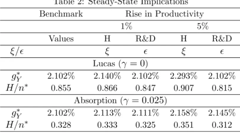
Table 2: Steady-State Implications
Benchmark Rise in Productivity
1% 5%
Values H R&D H R&D
ξ/ǫ ξ ǫ ξ ǫ
Lucas (γ = 0)
g∗
Y 2.102% 2.140% 2.102% 2.293% 2.102%
H/n∗ 0.855 0.866 0.847 0.907 0.815
Absorption (γ = 0.025) g∗
Y 2.102% 2.113% 2.111% 2.158% 2.145%
H/n∗ 0.328 0.333 0.325 0.351 0.312
8Withσ = 1 the impact of R&D in growth and welfare would be near null, because nwould not influence
The table shows that the consideration of absorption implies an impact of R&D productivity
in growth, as with the model without absorption, the growth rate remains equal between the
benchmark case and both cases with rises inǫ(2.102%). However, in the model with absorption
the effect of a change in R&D productivity is positive, being almost equal to the effect of a
change in human capital productivity. Increases in human capital accumulation productivity
naturally imply a rise in the equilibrium human capital to varieties ratio and increases in R&D
productivity imply a fall in the steady-state human capital to varieties ratio.
In the next section, we consider welfare effects taking all the transition dynamics into
ac-count. The effect on welfare of increasing productivities in human capital accumulation or R&D
cannot be directly driven from the steady-state effects as transitional effects may also influence
welfare and production.
3.3 The Influence of R&D and Human Capital in wealth and welfare taking
Transition into account
In order to present results that take in account the evolution of an economy with absorption,
we proceed as Brunner and Strulik (2002). First we backward integrate the three differential
equations that describe the transition applying the benchmark calibration described in the table
1. Then, we compare these results with four different exercises: a 1% rise in human capital
accumulation productivity (ξ); a 1% rise in R&D productivity (ǫ); a 5% rise in human capital
accumulation productivity (ξ) and a 5% rise in R&D productivity (ǫ).9 In all exercises, we
approximate the real interest rate (r0) and the human capital to varieties ratio (H/n0) from
the initial values obtained in the benchmark exercise, as these are predetermined variables.10
9A 5% rise in produtivities is equivalent to a new subsidy of 4.68%.
We first describe the transition path of most important variables in the “Lucas” model and
in the “Absorption” model. Then, we compare the impact of different productivities in output,
consumption and utility. The following figures describe the evolution of the “Lucas” economy
in the first 180 years.
0 50 100 150 0 0.005 0.01 0.015 0.02 0.025 time gY
0 50 100 150 0.06 0.08 0.1 0.12 0.14 time S h a re o f H i n R & D ( un )
0 50 100 150 0 0.002 0.004 0.006 0.008 0.01 0.012 time gn
0 50 100 150 4 5 6 7 8 9
x 10-3
time
g
H
0 50 100 150 0.062 0.063 0.064 0.065 0.066 0.067 0.068 time r
0 50 100 150 0.131 0.132 0.133 0.134 0.135 0.136 0.137 time C /K
0 50 100 150 0.019 0.02 0.021 0.022 0.023 time gC
The figure shows an oscillatory pattern of convergence as in G´omez (2005) and a lengthy
transition to the steady-state: the steady-state is not reached before 580 years.11 Next figures
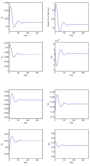
present the transition path of the absorption economy.
0 50 100 150 0.02 0.022 0.024 0.026 time gY
0 50 100 150 0.2 0.25 0.3 time S h a re o f H i n R & D ( un )
0 50 100 150 0 0.002 0.004 0.006 0.008 0.01 0.012 time gn
0 50 100 150 4 5 6 7 8 9
x 10-3
time
g
H
0 50 100 150 0.061 0.062 0.063 0.064 0.065 0.066 0.067 time r
0 50 100 150 0.131 0.132 0.133 0.134 0.135 0.136 time C /K
0 50 100 150 0.019 0.02 0.021 0.022 time gC
0 50 100 150 0.28 0.3 0.32 0.34 0.36 0.38 time H /n
Figure 2: Transition Paths for Representative Variables in the “Absorption” Calibration
The figure shows that the economy with absorption presents a shorter transition path,
reaching the steady-state near 150 years after the beginning. In this feature, this economy
seems to be more close to reality that the simpler “Lucas” economy. The economy maintains
the oscillatory pattern which can be characterized by an initial overshooting of the final values
for most variables.
Now, we want to compare the welfare effects of rising productivities in both models, in order
to demonstrate our claim according to which the model with absorption shows higher effects of
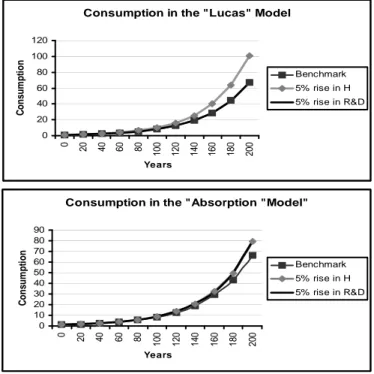
R&D policies than the simpler model. First we present two figures that show the evolution of
consumption in the first 200 years after the beginning (Figure 3). In order to keep the figures
clear, we only compare the benchmark case with the 5% rise in both parameters.
Consumption in the "Lucas" Model
0 20 40 60 80 100 120
0 20 40 60 80
10 0 12 0 14 0 16 0 18 0 20 0 Years C o n s u m p ti o n Benchmark 5% rise in H 5% rise in R&D
Consumption in the "Absorption "Model"
0 10 20 30 40 50 60 70 80 90
0 20 40 60 80
1
00 120 140 160 180 200
Years C o n su m p ti o n Benchmark 5% rise in H 5% rise in R&D
Figure 3: Consumption Paths in the “Lucas” and “Absorption” Calibration
The first figure (The “Lucas” Model) shows that while increasing the human capital
the consumption path almost equal to that with the initial value for research productivity. The
second figure shows that both human capital productivity rises and R&D productivity rises
move upward the consumption path. In fact, consumption paths of both human capital and
R&D rises are almost the same.
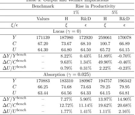
Next table shows values for output, consumption (calculated after 200 years) and utility for
each experiment.12
Table 3: Output and Welfare Implications
Benchmark Rise in Productivity
1% 5%
Values H R&D H R&D
ξ/ǫ ξ ǫ ξ ǫ
Lucas (γ = 0)
Y 171139 187980 172920 259061 170078
C 67.20 73.67 68.10 100.7 66.89
U 64.30 64.80 64.50 65.72 64.15
∆Y /Ybench – 8.22% 0.43% 51.89% -0.70%
∆C/Cbench – 9.63% 1.34% 49.90% -0.46%
∆U/Ubench – 0.79% 0.31% 2.22% -0.23%
Absorption (γ = 0.025)
Y 170883 183310 180967 194757 196342
C 66.25 74.68 73.63 79.25 79.95
U 63.44 64.56 64.33 64.15 64.81
∆Y /Ybench – 7.27% 5.90% 13.97% 14.90%
∆C/Cbench – 12.72% 11.14% 19.62% 20.68%
∆U/Ubench – 1.77% 1.41% 1.11% 2.16%
From the analysis of the table, we confirm that in the “Lucas” framework only human capital
productivity (policy) has significative effects in output, consumption and in utility. However,
in the “Absorption” model R&D productivity (policy) becomes as important or even more
important (in the 5% rise case) than human capital productivity (policy).
12According to (23), utility is calculated as Uss = Css1−θ−1
1−θ + gC
ρ
ρ−(1−θ)gC . As in the G´omez (2005) model, output is
4
Conclusions
We add to Arnold (1998, 2000) the consideration of absorption as a source of human capital
accumulation. We present the steady-state of the model, as well as simulated its transition
along a balanced growth path. This allowed for a dramatic increase in the effect of R&D when
compared to a more usual Lucas-type human capital accumulation. This article complements
that of Zeng (2003) as we calculate the complete transition path for the economy and focus
on output, consumption and welfare and not only on growth rates. Thus, these conclusions
indicate the relevance of future empirical research on the relative importance of absorption by
human capital accumulation in different economies.
References
[1] Arnold, L. (1998), “Growth, Welfare and Trade in an Integrated Model of Human-Capital
Accumulation and Research”,Journal of Macroeconomics,20(1), 81-105.
[2] Arnold, L. (2000), “Endogenous growth with physical capital, human capital and product
variety: A Comment”,European Economic Review, 44, 1599-1605.
[3] Barrio-Castro, T., E. L´opez-Bazo, and G. Serrano-Domingo (2002), “New Evidence on
International R&D spillovers, human capital and productivity in the OECD”, Economics
Letters, 77, 41-45.
[4] Brunner, M. and H. Strulik (2002), “Solution of Perfect Foresight Saddlepoint Problems: A
simple method and Aplications”,Journal of Economics Dynamics and Control,
[5] Eicher, T. (1996), “Interaction Between Endogenous Human Capital and Technological
Change”,Review of Economic Studies, 63, 127-144.
[6] Funke, M. and H. Strulik (2000), “On Endogenous growth with physical capital, human
capital and product variety”,European Economic Review, 44, 491-515.
[7] G´omez, M. (2005), “Transitional Dynamics in an Endogenous Growth Model with Physical
Capital, Human Capital and R&D”, Studies in Nonlinear Dynamics and Econometrics,
Vol. 9(1), Article 5. http://www.bepress.com/snde/vol9/iss1/art5.
[8] Iyigun, M. and Owen, A. (1999), “Entrepreneurs, Professionals and Growth”, Journal of
Economic Growth, vol. 4, number 2, 215-232.
[9] King, R. and Rebelo, S. (1993), “Transitional Dynamics and Economic Growth in the
Neoclassical Model”,American Economic Review, 83(4), September, 908-931.
[10] Jorgenson, D. and B. Fraumeni (1993), “Education and Productivity Growth in a Market
Economy”,Atlantic Economic Journal, vol. 21, issue 2, June, 1-25.
[11] Lucas, R. (1988), “On the Mechanics of Economic Development”, Journal of Monetary
Economics, 22, 3-42.
[12] Maddison, A. (1995), Monitoring the World Economy 1820-1992, Development Center
Studies, OECD, Paris.
[13] Peretto, P. (2003), “Fiscal Policy and Long-Run Growth in R&D based Models with
en-dogenous Market Structure”,Journal of Economic Growth, v.8, June, 325-347.
[15] Zeng, J. (2003), “Reexamining the interaction between innovation and capital
accumula-tion”,Journal of Macroeconomics 25, 541-560.
A
Appendix: Jacobian of the Linearized Systems
Linearizing the system (34), (33) and (31) around its steady-state (r∗, C/K∗, H/n∗), the
dy-namics can be approximated by the following third order system:
· r · C/K · H/n = ³
αη(1−α)
αβ−(1−α)η −
1−β−αη β
´
r∗ − η(1−α)
αβ−(1−α)ηr
∗ Ω
1
(1/θ−(1−αη)/β)C/K∗ C/K∗ 0
Ω2 Ω3 Ω4
r−r∗
C/K −C/K∗
H/n−H/n∗
(39)
where
Ω1 = (σ−1)(
H n)
σ−2σγα(1−β−η) + (1−α)η
αβ−(1−α)η r
∗; (40)
Ω2 =
1
1−1−ααβη +B1B2
·
1−αη β µ H n ¶∗¸ ; (41)
Ω3 = −
1
1−1−ααβη +B1B2
·
1−αη β µ H n ¶∗¸ ; (42)
Ω4 = (σ−1)γ
µ
(H n)
∗ ¶(σ−1)
+ξ(ξ+p)ǫ(1−β−η) (1−α)η
µ
H n
¶∗
−
−ξǫ(1−β−η)
(1−α)η σγ(σ−2)
µ
(H n)
∗ ¶(σ−2)
+gn∗
µ
H n
¶∗
1
ǫ. (43)
We are now able to calculate the eigenvalues for each one of the presented exercises. As we
have 2 predetermined variables we need two stable roots. In the “Absorption” Model - that
corresponds to the calibration in column (2) in Table 1, the real parts of the eigenvalues are
-0.0121, -0.0121 and 0.0267. Values for other exercises are available upon request. For ease of