Transitional Dynamics of an Endogenous
Growth Model with an Erosion Effect
Tiago Neves Sequeira
∗Dep. Gest˜ao e Economia, Universidade da Beira Interior
INOVA, Fac. Economia, Universidade Nova de Lisboa
Abstract
The convergence features of an Endogenous Growth model with Physical capital, Human Capital and R&D have been studied. We add an erosion effect (supported by empirical evidence) to this model, and fully characterize its convergence properties. The dynamics is described by a fourth-order system of differential equations. We show that the model converges along a one-dimensional stable manifold and that its equilibrium is saddle-path stable. We also argue that one of the implications of considering this “erosion effect” is the increase in the adherence of the model to data.
JEL Classification: O11, O15, O31, O33, O41.
Key-Words: endogenous growth models; convergence; erosion ef-fect; model fitness.
1
Introduction
Arnold (1998, 2000) built an endogenous growth model with physical capital, human capital and R&D and studied its convergence properties. Funke and Strulik (2000), in a similar model, showed that a developing economy evolves through different stages of development. As they failed to note that the interest rate was a predetermined variable in the innovative economy, as it depended directly on the human capital to knowledge ratio (a variable determined by history), G´omez (2005) derived the correct conditions for steady-state stability of the model.
In their model, Galor and Moav (2002:1148) introduce an “erosion ef-fect”: “Technological progress reduces the adaptability of existing human capital for the new technological environment”. In Galor’s (2005) model there is a positive association between human capital accumulation and tech-nological progress because rising levels of schooling lessen the adverse effect of technological change on human capital accumulation. Kumar (2003) and Tamura (2006) found, in econometric estimations, a negative influence of Total Factor Productivity (TFP) growth in human capital that questions this result (also present in Tamura’s own model).1 Tamura (2006:46) states
that “The evidence is unambiguous; young adult years of schooling is nega-tively related to the growth rate of TFP”. Sequeira and Reis (2006) used an “erosion effect” to explain the decreasing proportion of investment in high-tech skills in developed countries, a fact highlighted by Sequeira (2003). The intuition was that at least some types of human capital depreciates when dealing with new technologies. This article provided results of a calibration exercise in a more complex model with two accumulable stocks of human capital but did not characterize the conditions for saddle-path stability.2
Galor and Moav (2002:1148) also assume a “productivity effect”, according to which when an innovation occurs, each individual operates with a supe-rior level of technology. When comparing both effects, the author argued that “Once the rate of technological progress reaches a positive steady-state
1
In his theoretical model Kumar explains this feature of the data through the impact of the real interest rate on the decision of schooling; when the economy becomes more open, technology adoption increases, implying a rise in the real interest rate and thus, a decrease of human capital accumulation.
2
level, the erosion effect is constant, whereas the productivity effect grows at a constant rate”. These features are also present in this article.
We fully characterize a model of Endogenous Growth through physical capital, human capital and R&D with an “erosion effect” in human capi-tal accumulation. This is made solving a fourth-order differential equation system, in which only one variable is predetermined. The human capital ac-cumulation function used in the article predicts a positive relationship with schooling, a negative relationship with technological progress and a posi-tive effect of technological progress in returns to human capital (or broadly speaking in wage inequality), standard facts in Galor’s articles.
We find that the stability properties of this model with an “erosion ef-fect” increase its comparability to data when compared to the G´omez (2005) model without the “erosion effect”. In fact, the fulfillment of the conditions for saddle-path stability - stated in G´omez (2005) - implies a low substitu-tivity parameter in the differentiated good which implies a too large markup relative to data (see e.g. Noorbin, 1993). Furthermore, counterfactual os-cillatory dynamics for developed countries - along a two-dimensional stable manifold - arise for plausible parameter values.3 This oscillatory pattern
happened in variables for which history has shown a monotonic evolution, as the investment share in R&D and theper capita output growth rate (see e.g. Maddison, 1995, 2001; Jones, 1995 and Sφrensen, 1999).
This article intend to contribute to the understanding of the stability properties of endogenous growth models while adds to the discussion of their fitness to well-known evidence. We show that the introduction of the “erosion effect” improves the fitness of the model to data, allowing for more reasonable values for the markup that fulfil the saddle-path stability conditions and providing the monotonic convergence.4
In section 2, we present the model. In Section 3, we present the Balanced Growth Equilibrium and the stability analysis of the steady-state. In section 4, we calculate alternative growth paths that fit the stability conditions previously derived. Then we discuss the adherence of the model behaviour to evidence. In section 5, we conclude.
3
The author showed that the stable eigenvalues are likely to be complex.
4
2
The Model
This section recapitulates the Arnold’s (1998, 2000) - Funke and Strulik (2000) - G´omez (2005) model, assuming a different function for accumulation of human capital, which accounts for the existence of an “erosion effect”.
2.1
Setup of the Model
Consider a closed economy inhabited by a constant population, normalized to one, of identical infinitely-lived households that maximize the intertem-poral utility function:
Z ∞
0
C1−θ
1−θe
−ρt
dt, ρ >0, θ >0, (1)
(where C denotes consumption, ρ is the time-discount rate and θ is the relative risk aversion coefficient) subject to the budget constraint and the knowledge accumulation technology. Human Capital,H, can be devoted to production (HY), education (HH) and R&D (Hn), such that:
H =HY +HH +Hn, (2)
and is calculated according to:
·
H=ξHH −ϑgnH,5 (3)
where gn is the growth rate of the number of varieties and ϑ represents
the “erosion effect” in human capital caused by R&D. In Galor’s (2002, 2005) models the function of human capital accumulation implied a posi-tive relationship to schooling effort (HH in this model), a negative
relation-ship with technological progress (gn in this model) and a complementarity
between schooling and technological progress that allowed for an increase in technological progress to increase equilibrium education. Although this
complementarity is absent from (3) - ∂ ∂ · H/∂HH
∂gn = 0, the positive effect of
technological progress in the education effort is obtained (just divide (3) by
H and solve for HH
H , the allocation of human capital to education). R&D
technology is given by
·
n=ǫHn, (4)
5
whereǫ is the productivity of human capital in R&D. This process is possi-ble because of monopolistic competition in differentiated goods, as we will describe later. The budget constraint faced by the household is
·
W =rW +w(H−HH)−C, (5)
where r is the return per unit of aggregate wealth, W, and w the wage per unit of employed human capital. Letgz =
· z
z denote the growth rate of any
variablez. The first order conditions for maximization of (1), using (3) and (5) as constraints, give:
gC = (r−ρ)/θ (6)
gw = r−ξ+ϑgn. (7)
Equation (7) highlights one of the most important facts relating technology to human capital: the positive influence of technological progress in the returns to education (see Galor, 2005:58 and Eicher, 1996:132).
A single homogeneous final goodY is produced with Cobb-Douglas tech-nology
Y =A1KβDηH1
−β−η
Y , A1 >0, β > 0, η >0, β+η <1, (8)
whereK is physical capital,HY is human capital allocated to the final good
production andD is an index of differentiated goods,
D=
·Z n
0
xαidi
¸1/α
, 0< α <1, (9)
where substitutivity between varieties is measured byαandxiis the amount
used for each variety of then intermediate goods. The market for the final good is perfectly competitive and its price is normalized to one. Profit maximization gives the following inverse factor demands:
r= βY
K , (10)
PD =
ηY
D , (11)
w= (1−β−η)Y
HY
, (12)
where PD represents the price index for intermediates. The right
hand-side of (12) is the human capital productivity in the final good production. SubstitutingY by (8) and using (9), we can see the “productivity effect”.
Each firm in the differentiated-goods sector owns a patent for selling its variety xi. Let vt denote the expected value of innovation, defined by
vt=
Z ∞
t
e−[R(τ)−R(t)]
π(τ)dτ , where R(t) =
Z t
0
r(τ)dτ . (13)
Taking into account the cost of innovation as implied by (4), free entry conditions in R&D are defined as follows:
w/ǫ > v if n. = 0 (Hn= 0). (14)
w/ǫ=v if n >. 0 (Hn>0) or (15)
Finally, no-arbitrage requires that the valorization of the patent plus profits is equal to investing resources in the riskless asset:
·
v+π =rv ⇔
·
v
v =r−π/v. (16)
Producers act under monopolistic competition and maximize operating profits
πi = (Pxi −1)xi. (17)
The variablePxi denotes the price of an intermediate and 1 is the unit cost
ofY. From profit maximization in the intermediate-goods sector, each firm charges a price
Pxi = 1/α. (18)
With identical technologies and symmetric demand, the quantity supplied is the same for all goods, xi =x. Hence, equation (9) simplifies to
D=n1/αx. (19) FromPDD=pxntogether with equations (18) and (19) we obtain the total
X =xn=αηY. (20) After insertion of equations (18) and (20) into (17), profits can be rewrit-ten as a function of aggregate output and the number of existing firms:
π= (1−α)ηY /n. (21) Before we proceed with the analysis we compute some equations that will be useful. Insertion of equation (20) in the resource constraint
·
K =
Y −Rn
0 xidi−C simplifies it to
·
K = (1−αη)Y −C (22) and insertion of (19) and (20) in the production function (8) gives:
Y1−η
=A1(αη)ηKβnη
1−α α (u
1H)1
−β−η
, (23)
where u1 = HHY is the proportion of human capital employed in the final
good production.6 After time-differentiate the previous function we obtain
the following output growth rate:
(1−η)gY =βgK+ [
1−α
α ]ηgn+ (1−β−η)(gu1 +gH). (24)
Log-differentiation of equations (10) and (12) provides
gr =gY −gK, (25)
gw =gY −(gu1 +gH). (26)
We will concentrate in the innovative economy description. To avoid excessive length we refer to G´omez (2005) for the description of the stage with human and physical capital accumulation. In fact, as the change we introduce is due to R&D, that stage remains equal to the developing economy stage in that reference and in Funke and Strulik (2000). In the simulation of the model, we include this stage.
6
We will denoteu2=HHn the share of human capital in R&D andu3=HHH the share
2.2
The Innovative Economy
The fully industrialized economy is characterized by the presence of both hu-man capital accumulation (
·
H >0) and R&D (n >· 0). The following system of differential equations describes the dynamics of the fully industrialized economy:
gχ =
µ
1
θ −
1−αη β
r+χ− ρ
θ, (27)
gr = −
1−β−η
β (r−ξ) + η1−α
α −ϑ(1−β−η)
β gn. (28)
whereχ=C/K. It is worth noting that gn is no longer given as a function
of χ and r that could be substituted in previous equations, as in previous contributions (see e.g. G´omez, 2005:5). Departing from (15) and (16), we note thatgv =gw and that gw =r−ǫπ/w. Then, using (7), (12) and (21)
in this equation and solving to u1, we reach:
u1 =
(1−β−η)(ξ−ϑgn)
(1−α)ǫηψ . (29)
whereψ =H/n. Using (3) and (29), we reach the growth rate of ψ :
gψ =ξ
µ
1−
·
(1−β−η)(ξ−ϑgn)
(1−α)η +gn
¸
1
ǫψ
−(1 +ϑ)gn, (30)
Equation (29) implies thatgu1 =gn−gH − ϑ · gn
(ξ−ϑgn). Then, by (26), we note
that gu1 =gY −gw−gH. Then, using (25),gK from (22) and (7), we reach
the equation that describes the evolution of gn:
·
gn=
ξ−ϑgn
ϑ
·
(1 +ϑ)gn−
1−αη
β r+χ+ (r−ξ)−gr
¸
, (31)
where gn 6= ξϑ. Thus, the system constituted by equations (27), (28), (30)
3
The Balanced Growth Equilibrium and its
Stability
In this section, we present the balanced growth equilibrium and its stability. The next theorem states that the model has a positive long-run steady-state.
Theorem 1 Under usual restrictions in parameters, there is an unique posi-tive steady-state of the model given by (r∗
, χ∗
, ψ∗
, g∗
n) that is obtaining solving
the system of equations (27)-(30) and (31) to the steady-state:7
r∗
=
¡
η1−α
α + (1−β−η)
¢θξ−ρ
1+ϑ + (1−β−η)ρ
(1−β−η)−(1−θ)
1+ϑ
¡
η1−α
α + (1−β−η)
¢; (32)
χ∗
=
µ
1−αη β − 1 θ ¶ r∗ +ρ
θ; (33)
ψ∗
= ξ[g
∗
n(1−α)η+ (1−β−η)(ξ−ϑg
∗
n)]
(1−α)ηǫ(ξ−(1 +ϑ)g∗
n)
; (34)
g∗
n =
r∗
(1−θ) +θξ−ρ
θ(1 +ϑ) . (35)
Proof. The shares of human capital to different sectors must be constant for an interior steady-state solution. With u∗
1 and u
∗
3 constant, g
∗
n and ψ
∗
must be constant, by (4) and (29). Thusg∗
H =g
∗
n. Thus,g
∗
H is also constant.
From constancy of ψ∗
and u∗
1 we can say that g
∗
Y = g
∗
K. This equality,
equation (24) and the constancy of g∗
n, g
∗
H and u
∗
1 imply that r, g
∗
Y and
g∗
K are constant. Thus χ
∗
= (C/K)∗
is constant (to see this divide (22) by K). The conditions θ +ϑ > (1−θ)A2 and θξ > A21+−A2ϑρ (where A2 =
η
(1−β−η)
1−α
α ) guarantees that r
∗
is positive. χ∗
>0 if and only ifθξ > A3ρ,
where A3 =
(1+A2)
1+ϑ (
1−αη β −1)−
1−αη β
(1+A2)
1+ϑ (
1−αη
β −
1
θ)
.8 The necessary and sufficient condition
for g∗
n > 0 is θξ >
θ(1+A2)
θ(1+A2)+(1+ϑ)ρ. Condition ξ > (1 + ϑ)g
∗
n implies that
ξ > ϑg∗
n, for a positive g
∗
n. This condition implies that some human capital
is allocated to the final good production, which must be verified (see (29)) by the transversality condition onH.9 Both conditions guarantee the positivity
7
We detail sufficient and necessary conditions on positivity in the proof.
8
It is easy to see that withθ >1,ξ > ρthis condition is fulfilled. Note that 1−αη
of ψ∗
. With ξ > ρ and θ > 1 these conditions are always verified (as in G´omez, 2005).10
3.1
Stability
We will now analyze the dynamics of the model in the neighborhood of the steady-state. As usually, we can assume that the stocks of physical capital, human capital and the number of varieties move sluggishly, so that K(0), H(0) andn(0) are given by their historical values. Thus ψis predetermined. In Gom´ez (2005), as u1 is only dependent on ψ, it is also predetermined.
With a predeterminedu1, using (10) and (23), it becomes clear thatrshould
be predetermined. In consequence, in order to achieve stability in a model with two predetermined variables, Gom´ez (2005) found conditions for the existence of two stable eigenvalues. In our model u1 is not only dependent
on ψ, but also on gn (see (29)). Thus r is dependent both on ψ and on
gn. As gn is dependent on χ = C/K, gn can jump and r can also jump.
Other way to see that gn can jump is that it is dependent on a share of
human capital, a variable that is dependent on agents’ decisions. Thus to ensure local saddlepoint stability of the steady-state, we need one stable and three unstable eigenvalues. The analysis of the linearized system around the steady-state will establish that the stable-manifold is one-dimensional and the initial conditions determine the starting point in this stable manifold.
Linearizing the system of eq. (27)-(30) and (31) around its steady-state (r∗
, χ∗
, ψ∗
, g∗
n) gives the following fourth-order system:
lim
t→∞e
−ρt
λ2(t)H(t) = 0 (36)
(where λ2 is the co-state of H), which converts into
µ
−ρ+
·
λ2
λ2 +
· H H
< 0. As
·
λ2
λ2 =
ρ−ξ+ϑgnand
· H
H given by (3), the transversality condition is equivalent toξ >(1 +ϑ)g
∗
n.
10
· r · χ · ψ · gn =
−1−β−η
β r
∗
0 0 B1r∗
³
1
θ −
1−αη
β
´
χ∗
χ∗
0 0
0 0 ξ−ϑg∗
n−g
∗
n B2−(1 +ϑ)ψ
∗
−ξ−ϑg∗n
ϑ
(1−α)η
β
ξ−ϑg∗n
ϑ 0 −B3g
∗
n−B4ϑgξ∗
n
r−r∗
χ−χ∗
ψ−ψ∗
gn−g∗n
,
whereB1 =
η1−α
α −ϑ(1−β−η)
β ; B2 =ξϑ
(1−β−η) (1−α)η
1
ǫ − ξ ǫ;
B3 =
µ
(1 +ϑ)− η
1−α
α −ϑ(1−β−η)
β
;
B4 =
µ
χ∗
−1−η
β ξ−
(1−α)η β r
∗ 
. (37)
orx· =J(x−x∗
), whereJ is the Jacobian in (37). To demonstrate the con-ditions under which the system is saddle-path stable we state the following theorem.
Theorem 2 In the conditions of Theorem 1 and if ϑ > η1−αα−β
1−η is verified, there exists a one-dimensional stable Manifold tangent to the steady-state defined above in which any point converges to the steady-state.
The proof makes use of two lemmas that demonstrate that there are only one stable root if some conditions are verified. The necessary and sufficient conditions are determined within the proofs of the Lemmas.
Lemma 1 There is an uneven number of stable roots, one or three.
Proof. Lemma 1 is implied by a negative determinant of (37). There is one eigenvalue (e1 = ξ−ϑgn∗ −g
∗
n) that is always positive for a positive
steady-state as it is implied by the transversality condition on H (see the proof of Theorem 1). Thus, the sign of the determinant is negative if and only if:
·
B3g
∗
n+B4
ξ ϑg∗
n
¸
1−β−η β +
µ
1
θ −1−
1−β−η β
B1g
∗
n<0. (38)
The inequality (38) is equivalent to−1−β−η
(1+ϑ)−(1−1)η1−α
derived in Theorem 1 which ensured positiveness of r∗
. Thus, for a positive steady-state, the determinant of the Jacobian is always negative, implying that the steady-state can be saddle-path saddle (1 negative root) or the balanced growth path can be indeterminate (3 negative roots).
The following Lemma establishes the conditions according to which the steady-state is stable in the steady-state sense.
Lemma 2 There are not three stable roots.
Proof. Ase1is always positive for a positive steady-state, if there were 3
negative eigenvalues, the sum of these three roots cannot be positive. Thus we search for conditions according to which the sum of the remaining three eigenvalues is positive. We know that the trace ofJ in (37) is the sum of the all roots (T r(J) =e1+e2+e3+e4). Consequently,T r(J)−e1 =e2+e3+e4.
IfT r(J)−e1 >0, we cannot have three negative roots. The verification of
this condition gives
·
1− 1
θ +
1−α β η
¸
r∗
−
µ
B3g
∗
n+B4
ξ ϑg∗
n
+ρ >0. (39)
which is the necessary and sufficient condition for a saddle-path stability. A sufficient condition would be B3gn∗ +B4ϑgξ∗
n < 0. Noting that B4 =
−B3gn∗ (see eq. (31)) that expression in the steady-state yieldsϑ > η1−α
α −β 1−η .
Lemmas 1 and 2 prove that, under the derived condition, there is only one stable root, which proves saddle-path stability. Note that condition (39) is the necessary and sufficient condition for saddle-path stability.
We can note that as θ and ϑ become smaller, (39) is more difficult to obtain. Thus, it is possible that the system yields three stable roots, which would imply that the initial condition could not determine the initial point in the stable manifold. Thus different stable paths, depending on the jump variables, would converge to the steady-state.11
With usual calibration parameters, we reach one stable real eigenvalue and three unstable roots, as the condition stated in Lemma 2 is easily veri-fied. It is straightforward to show that with one predetermined value, it is possible to calculate the initial valuesr(0), χ(0),andgn(0) even ifψ(0)6=ψ
∗
using the eigenvector associated to the stable root. Thus ψ(0) determines the initial point in the one-dimensional stable manifold.
11
4
Adjustment Paths for Plausible
Calibra-tion Values
We present three different calibrations and compute the adjustment paths for each of them by backward integration (Brunner and Strulik, 2002). The first calibration is taken from Funke and Strulik (2000), the second is taken from Gom´ez (2005) and the third considers a higher α. The computation of the transition path was done in the form described by Gom´ez (2005) in order to avoid jumps between the two stages of development.12 The additional
parameter ϑ was calibrated as in Sequeira and Reis (2006), using evidence from Kumar (2003): ϑ= 0.268.
As we have noted earlier, the balanced growth path may be indetermi-nate. However, we center the analysis in calibrations that yield saddle-path stability, as they arise with most plausible parameters values.13 Calibration
1 assumes the following values: β = 0.36; η = 0.36; α = 0.4; ξ = 0.05;
ρ = 0.023; θ = 2; δ = 0.1. Calibration 2 assumes β = 0.36; η = 0.36;
α = 0.54; ξ = 0.05; ρ = 0.023; θ = 2; δ = 0.1. Calibration 3 is the fol-lowing: β = 0.36; η = 0.36; α = 0.74; ξ = 0.05; ρ = 0.023; θ = 2;
δ = 0.1. For the Calibration 1, eigenvalues are: 0.0418; 0.0898 + 0.1146i; 0.0898−0.1146i;−0.1056; for calibration 2 they are 0.0398; 0.1221+0.0830i; 0.1221−0.0830i;−0.0667 and finally for calibration 3 they are 0.0374; 0.1891; 0.1050; −0.0445.
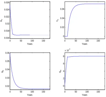
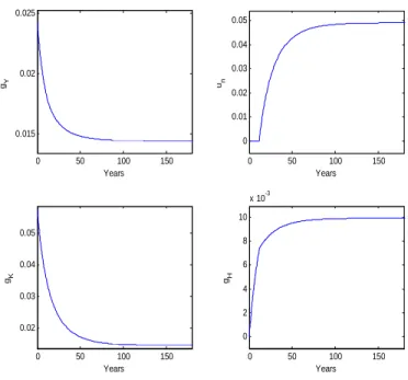
Figures 1 to 3 show adjustment paths of the growth rate of output and capital and the share of human capital allocated to research for each of the calibrations.14
12
See G´omez (2005:14) for a discussion on the issue.
13
Withθ= 1 andϑ <0.051 (withβ = 0.36;η= 0.36;α= 0.4;ξ= 0.05;ρ= 0.023 and
δ = 0.1 - the typical calibration in G´omez, 2005), we reach three negative eigenvalues, two of them complex conjugates.
14
We only show adjustment paths forgY ,un=Hn/H,gK andgH to focus the article.
0 50 100 150 0.016
0.018 0.02 0.022 0.024 0.026
Years
gY
0 50 100 150 0
0.02 0.04 0.06 0.08
Years
un
0 50 100 150 0.02
0.03 0.04 0.05
Years
gK
0 50 100 150 0
2 4 6 8
x 10-3
Years
gH
Figure 1: Transition Paths for Representative Variables (Calibration 1)
0 50 100 150 0.016
0.018 0.02 0.022 0.024 0.026
Years
gY
0 50 100 150 0
0.02 0.04 0.06
Years
un
0 50 100 150 0.02
0.03 0.04 0.05 0.06
Years
gK
0 50 100 150 0
2 4 6 8
x 10-3
Years
gH
0 50 100 150 0.015
0.02 0.025
Years
gY
0 50 100 150 0
0.01 0.02 0.03 0.04 0.05
Years
un
0 50 100 150 0.02
0.03 0.04 0.05
Years
gK
0 50 100 150 0
2 4 6 8 10
x 10-3
Years
gH
Figure 3: Transition Paths for Representative Variables (Calibration 3)
These figures show that adjustment equilibrium paths are monotonic, contrary to what happened in G´omez (2005).15 In the following section we
discuss the adherence to data of these results.
4.1
The Model versus Evidence
reaches 20% 20 years after the beginning of the R&D stage (which is clearly unrealistic), reaches near 1%, 15 years later, and reaches 6% after 180 years the beginning of the transition.
The steady-state growth rate of per capita output is between 1.4% and 1.8%, depending on calibration, which is a quite reasonable value for the industrialized world. Moreover, in the first two calibration exercises, the entrance in the R&D stage acts in order to increase the economic growth rate, which seems to have occurred. According to Maddison (2001), growth rates in the USA were 1.43% (1820-90); 1.83% (1890-1929); 1.96% (1929-80) and 2.17% (1980-98).16 We note that in the simulation presented in G´omez
(2005), the economic growth rate was near 1.8% in the beginning of the R&D stage, 2.4% twenty years later and near 2.1% after 180 years the beginning of the transition. Although the steady-state values for these variables are in line with data in G´omez (2005) baseline scenario, the oscillatory patterns do not seem so.
Finally, one of the most relevant data implications of G´omez (2005) sta-bility restrictions on parameters is a non-realistic high value for the markup (α = 0.4 implies a markup of 2.5). Norrbin (1993) presented markups for sectors in the USA, all below 1.84. A α = 0.54 implies a markup of 1.85 and a α = 0.75 implies a markup of 1.33. These smaller markups, now in line with data, satisfy the stability conditions derived above.
5
Conclusion
We introduce an “erosion effect” to the human capital accumulation technol-ogy in the innovative economy described by Arnold (1998, 2000) and Funke and Strulik (2000) following the empirical contributions of Kumar (2003) and Tamura (2006) and following the ideas of Galor (2005) and Sequeira and Reis (2006, 2007). We have derived the convergence properties of the model. In particular, the stability analysis reveals that, with reasonable parameters values, this model is saddle-path stable and converges along a one-dimensional stable manifold.
With this, we show that the presence of this “erosion effect” contributes to increase the fit of an endogenous growth model with physical capital, human capital and R&D to well-known evidence for a leader economy. This is obtained due to three features that are dependent on the “erosion effect”.
16
First, the “erosion effect” implied that r is not predetermined (as in the G´omez’ model), which imply that saddle-path stability is obtained with one stable root. Second, this stable root is real and thus the model shows a monotonic transition towards the steady-state. Third, a realistic markup can respect the stability conditions, for reasonable values of the other pa-rameters.
References
[1] Arnold, L. (1998), “Growth, Welfare and Trade in an Integrated Model of Human-Capital Accumulation and Research”, Journal of Macroeco-nomics, 20(1), 81-105.
[2] Arnold, L. (2000), “Endogenous growth with physical capital, human capital and product variety: A comment”,European Economic Review, 44, 1599-1605.
[3] Benhabib, J. and R. Perli (1994), “Uniqueness and Indeterminacy: On the Dynamics of Endogenous Growth”, Journal of Economic Theory,
63, 113-142.
[4] Brunner, M. and H. Strulik (2002), “Solution of Perfect Foresight Sad-dlepoint Problems: A simple method and Aplications”,Journal of Eco-nomics Dynamics and Control, 25(5):737-753, May.
[5] Carrillo, M. and A. Zazzaro (2000), “Innovation, Human Capital De-struction and Firms’ Investment in Training”, The Manchester School, 68, 3, 331-348.
[6] Eicher, T. (1996), “Interaction Between Endogenous Human Capital and Technological Change”,Review of Economic Studies, 63, 127-144.
[7] Funke, M. and H. Strulik (2000), “On Endogenous growth with phys-ical capital, human capital and product variety”, European Economic Review, 44, 491-515.
[10] G´omez, M. (2005), “Transition Dynamics in an Endogenous growth model with physical capital, human capital and R&D”,Studies in Non-linear Dynamics & Econometrics, 9, 1, Article 5.
[11] Kumar, K. (2003), “Education and Technology Adoption in a Small Open Economy: Theory and Evidence”,Macroeconomic Dynamics, vol. 7, 586-617.
[12] Jones, C. (1995), “R&D-based models of endogenous growth”,Journal of Political Economy, vol. 103, n.4, 759-584.
[13] Maddison, A. (1995), Monitoring the World Economy 1820-1992, De-velopment Center Studies, OECD, Paris.
[14] Maddison, A. (2001),The World Economy, a millenial perspective, De-velopment Center Studies, OECD, Paris.
[15] Norrbin, S. (1993), “The Relation between Price and Marginal Cost in U.S. Industry: A contradiction”, Journal of Political Economy, vol. 101, 6, pp. 1149-1164.
[16] Sequeira, T. N. (2003), “High-Tech Human Capital: Do the Richest Invest the Most?”, Topics in Macroeconomics, The Berkeley Journals in Macroeconomics, vol.3: n. 1, Article 13. http://www.bepress.com/bejm/topics/vol3/iss1/art13.
[17] Sequeira, T. N. and A. Reis (2006), “Human Capital Composition, R&D and the Increasing Role of Services”,Topics in Macroeconomics, The Berkeley Journals in Macroeconomics, vol.6: n. 1, Article 12. http://www.bepress.com/bejm/topics/vol6/iss1/art12
[18] Sequeira, T. N. and A. Reis (2007),Human Capital and Overinvestment in R&D, Scandinavian Journal of Economics, forthcoming.
[19] Sφrensen, A. (1999), “R&D, Learning and Phases of Economic Growth”,Journal of Economic Growth, 4, 429-445, December.
[20] Tamura, R. (2006), “Human Capital and Economic Development”,