INTRODUCTION
A major concern in maize breeding is to identify genes that control disease resistance, and this may be done using molecular markers. The general strategy involves geno-typing individuals from a segregating population with molecular markers scattered throughout the genome and measuring the disease resistance of their progeny. Statis-tical methods are then used to establish associations between changes in allelic states at the marker-loci and quantitative variations in resistance. A marker is said to be linked to a quantitative trait locus (QTL) when a significant association is demonstrated.
Currently, the two basic approaches to QTL mapping are: single-marker analysis and interval mapping. In the former, statistical analysis is applied to each marker-locus in a one-at-a-time fashion, while in the latter the joint frequencies of genotypes at two adjacent marker loci are used to infer the genotypes at the QTL. Single-marker analysis is a simple approach and has been used extensively in mapping, and for learning the principles of QTL mapping. This analysis can be implemented as a simple t-test, analysis of variance, linear regression, and likelihood tests (Liu, 1998). However, in some cases the underlying assumptions
of these tests are not met because of heteroscedasticity, non-linearity, and non-normality of residuals. For instance, plant pathologists often use visual ratings of disease severity obtained from individual plants as an estimate of the degree of resistance. Generally, these ratings consist of an ordinal scale that varies from 1 (resistant) to 9 (susceptible).
Ordinal data can be analyzed using ordinal categorical response techniques (Agresti, 1984). The advantage of using these techniques compared to traditional tests of asso-ciation is that the models allow the inclusion of assoasso-ciation terms without saturation, that is, the models do not require all the degrees of freedom. Furthermore, it is possible to construct more parsimonious models and also detect marker-locus associations in addition to describingcertain trends which are biologically meaningful based on para-meters. These parameters are the odds ratio, which are easy to interpret (Agresti, 1984).
When applied to the mapping of disease resistance genes, the data consist of counts or frequencies arranged in multinomial contingency tables formed by cross classification of the response variable or disease severity levels (columns) and the explanatory variables or genotypes of the marker-locus under investigation (rows). The data may involve Poisson, multinomial or product multinomial
Proportional odds model applied to mapping of disease resistance genes in plants
*Maria Helena Spyrides-Cunha1, Clarice G.B. Demétrio2 and Luis E.A. Camargo3
Abstract
Molecular markers have been used extensively to map quantitative trait loci (QTL) controlling disease resistance in plants. Mapping is usually done by establishing a statistical association between molecular marker genotypes and quantitative variations in disease resistance. However, most statistical approaches require a continuous distribution of the response variable, a requirement not always met since evaluation of disease resistance is often done using visual ratings based on an ordinal scale of disease severity. This paper discusses the application of the proportional odds model to the mapping of disease resistance genes in plants amenable to expression as ordinal data. The model was used to map two resistance QTL of maize to Puccinia sorghi. The microsatellite markers bngl166 and bngl669, located on chromosomes 2 and 8, respectively, were used to genotype F2 individuals from a segregating population. Genotypes at each marker locus were then compared by assessing disease severity in F3 plants derived from the selfing of each genotyped F2 plant based on an ordinal scale severity. The residual deviance and the chi-square score statistic indicated a good fit of the model to the data and the odds had a constant proportionality at each threshold. Single-marker analyses detected significant differences among marker genotypes at both marker loci, indicating that these markers were linked to disease resistance QTL. The inclusion of the interaction term after single-marker analysis provided strong evidence of an epistatic interaction between the two QTL. These results indicate that the proportional odds model can be used as an alternative to traditional methods in cases where the response variable consists of an ordinal scale, thus eliminating the problems of heterocedasticity, non-linearity, and the non-normality of residuals often associated with this type of data.
*Part of a thesis presented by M.H.S.-C. to the ESALQ/USP, in partial fulfillment of the requirements for the M.Sc. degree. 1Departamento de Estatística, UFRN, Campus Universitário, s/n, Caixa Postal 1615, 59072-970 Lagoa Nova, Natal, RN, Brasil.
Send correspondence to M.H.S.-C. E-mail: [email protected]
2Departamento de Matemática e Estatística, ESALQ/USP, Caixa Postal 9, 13418-900 São Paulo, SP, Brasil. E-mail: [email protected] 3Departamento de Fitopatologia, ESALQ/USP, Piracicaba, SP, Brasil. E-mail: [email protected]
distributions. The most appropriate method for modelling counts is the Poisson regression model, which is a parti-cular case of the generalized linear models, developed by Nelder and Wedderburn (1972). McCullagh and Nelder (1989) showed that multinomial and product multinomial distributions can be derived from a set of independent Poisson random variables so long as their totals are fixed. Particular cases occur when the response categories are ordered. McCullagh (1980) suggested that the proportional odds and proportional hazard models should be used to analyze such data. These approaches are based on cumulative response probabilities and are multivariate extensions of generalized linear models.
This paper describes the application of the propor-tional odds model in mapping disease resistance QTL in maize. Some of the experimental data used in this analysis have been published elsewhere (Camargo et al., 1998).
MATERIAL AND METHODS
The model
Consider a multidimensional table with counts Yij, where i = 1,…,r and j = 1,…,c. Suppose that the columns are the ordinal response categories and that one is interested in comparing rows, i.e., the populations formed by combination of the levels of explanatory variables.
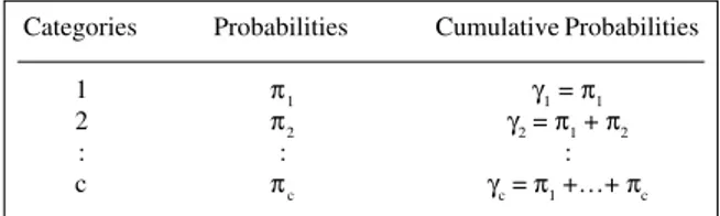
In such a contingency table, three types of sampling schemes can be obtained, e.g., Poisson, multinomial and product multinomial, depending on the constraints imposed on the parameters of the model. For the purpose of estimation, the Poisson distribution can be considered in all cases. Since the Poisson process belongs to the family of exponential distributions, such a problem can be treated as a generalized linear model (GLM). To define a GLM, three elements need to be identified: a probability dis-tribution, a linear model and a link function (Demétrio, 1993). Maximum likelihood (ML) estimates can be obtained by iterative methods such as the iterative reweighted least squares method, which is found in the major statistical packages, such as GLIM4 (Payne, 1986), SAS (1988) and others. McCullagh (1980) showed how to use the Newton-Raphson method for ML estimation in a class of models that includes cumulative logit models. For ordinal response scales, it is more suitable to form the link function using the cumulative probabilities γ
j =
P(Y ≤ j) (Table I) instead of the response category probabilities because of the former’s useful properties (McCullagh and Nelder, 1989). Wolfe (1996) developed a macro ORDINAL in GLIM4 to obtain estimates of such models.
Thus, the proportional odds model is defined by:
L
j(i) = log = αj + β
Tx
i
which can be written as row effects:
L
j(i)= log = αj + τi
where ∑τ
i = 0, αj represents the threshold of the underlying
continuous variable marking the boundaries between categories of the response and α
1<α2<…<αc-1, Lj(i)is the cumulative logit used as a link function, β or τ
i are the
parameter vectors and x
i represents the covariates in the
model or design matrix.
Parameter interpretation
The β parameter can be interpreted as the logarithm of the odds ratio such that the difference between the logits L
j(b)and Lj(a), for each pair of rows of the contingency table,
a and b, is the log of the local-global odds ratio θ
ij. Thus
L
j(b)- Lj(a)= log = log(θij) = β (1)
In other words,
θij = eβ.
The thresholds α
j are ordinarily considered to be
in-cidental parameters of little interest in themselves (McCullagh and Nelder, 1989). They can be interpreted as threshold parameters for the distribution of an unobserved continuous latent variable.
The statistical significance of the association between the response and the explanatory variables can be assessed by testing H
0:β = 0 or H0:τi = 0 or, in terms of odds ratios,
as H
0:θij = 1. Thus, if θij = 1, then the variables are not
associated. When 1 ≤θ
ij<∞, the individuals in row b have
a greater propensity to produce a lower response than individuals in row a of the explanatory variable, whereas when 0 ≤θ
ij< 1, the individuals in row b are less likely to
produce a lower category response than individuals in row a of the explanatory variable.
Table I - Cumulative probabilities of the ordinal categories. Categories Probabilities Cumulative Probabilities
1 π1 γ1 = π1
2 π2 γ2 = π1 + π2
: : :
c πc γc = π1 +…+ πc
j = 1, ..., c-1.
γj(i) 1 - γ
j(i)
γj(i) 1 - γj(i)
γb 1 - γb
γa 1 - γ
The proportional odds model described by McCullagh (1980) owes its name to the fact that it assumes that the log of the odds ratio is proportional to the distance between the values of the explanatory variables, with a constant proportionality at each threshold. This means that there is a single common slope parameter for each of the expla-natory variables, i.e., a hypothesis of parallelism where H
0:β1 = β2 =…= βj = β. Hosmer and Lemeshow (1989) use
the score test to verify this hypothesis.
After parameter estimation by the ML method, the estimated logits can be obtained and, by inversion, the esti-mated expected frequencies of each cell can be computed as:
γj(i) =
Hypotheses about the β parameters can be tested using the Wald statistic given by:
W = β’V-1β
which has the χ2 distribution and V-1 is the estimated
information matrix.
Goodness-of-fit
Nelder and Wedderburn (1972) suggested that deviance should be used to test a hypothesis of independence. The residual deviance is a measure of goodness-of-fit, which gives an overall indication of the fit of the model. A large value for this statistic is a clear indication of a substantial problem with the model. The goodness-of-fit is computed using the log of the likelihood-ratio. For contingency table cases in which the frequencies follow a Poisson distri-bution, this statistic is given by:
G2 = 2∑∑ y
ij log .
Under the null hypothesis, i.e., that independence is true, G2 has an asymptotic chi-squared distribution with
(r-1)(c-1) degrees of freedom.
To assess the effect of an explanatory variable, terms are sequentially included in the model and the deviance is measured at each step. Thus, the difference between the deviance of the independence model (I) and the deviance of the current model (C) will be:
G2(I/C) = G2(I) - G2(C) ~ χ2 df
with degrees of freedom (d.f.) given by the difference between the number of logits and the number of adjusted parameters. The number of logits is r(c-1) since for each row there are c-1 logits.
Case study
The experimental data used in the following analysis were collected from an ongoing project of mapping the disease resistance genes of maize to Puccinia sorghi, the causal agent of common rust. Some of the results of this project have been published elsewhere (Camargo et al., 1998). Data from one field trial were re-analyzed using the proportional odds model. The mapping strategy consisted of genotyping 97 F
2 plants derived from a cross
between the resistant L10 and the susceptible L20 inbred lines with the microsatellite marker-loci bngl166 and bngl669 which map to chromosome 2 and 8, respectively (Taramino and Tingey, 1996). The F
2 plants were
self-pollinated to generate F
3 progeny which were evaluated for
resistance to P. sorghi in a field trial. The experimental design consisted of a randomized complete block design with three blocks using a fully crossed factorial treatment scheme. The plots consisted of 10 plants per progeny grown in 2.5-m long rows spaced 0.8 m apart. Parental lines and hybrids were included as control treatments.
The plants were infected naturally and visual ratings of disease severity were made 1-2 weeks after flowering on a scale of 1 to 9, where 1 corresponded to no symptoms and 9 to more than 75% of the leaf area affected by the disease. To apply the ordinal categorical data method, the disease severity level of each plot, and not of each plant, was considered the response variable.
The proportional odds model applied to the experi-mental data can be written as:
log = α
j + τ
L1 + τL2 + τL1*L2
1 ≤ i ≤ 3; 1 ≤ k ≤ 3 1 ≤ j ≤ 5 - 1
where ∑τL1 = 0, ∑τL2 = 0 and ∑τL1*L2 = 0, α
j represents the
jth threshold, τL1 is the ith locus bngl669 level effect on
the severity of common rust, τL2 is the kth locus bngl166
level effect on the severity of common rust and τL1*L2 is the
interaction effect.
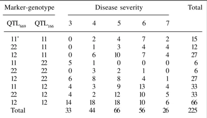
Although the scale for the severity of disease varied from 1 to 9, there were no extreme values so that scores of 1 to 3 and 7 to 9 were condensed, resulting in c = 5 response classes. Since the genotypes of some progenies could not be identified, the number of observations was reduced to 225 points.
RESULTS AND DISCUSSION
The frequencies of each cell and the jth cumulative probabilities at each level of disease severity relative to microsatellite-marker genotypes are shown in Table II and Figure 1, respectively.
Plant homozygous for L10 alleles at bngl669 and
1
i j
y ij
m ij
^
((
exp(L
j(i))
[exp(L
j(i)) + 1]
^ ^ ^
^ ^
γj(i,k) 1 - γ
j(i,k)
i k ik
i k ik
i
k
Table II - Observed frequencies of marker genotypes in each cell of the contingency table.
Marker-genotype Disease severity Total
QTL669 QTL166 3 4 5 6 7
11* 11 0 2 4 7 2 15
22 11 0 1 3 4 4 12
12 11 0 6 10 7 4 27
11 22 5 1 0 0 0 6
22 22 0 3 2 1 0 6
12 22 6 8 8 4 1 27
11 12 4 3 9 13 4 33
22 12 4 2 12 10 5 33
12 12 14 18 18 10 6 66
Total 33 44 66 56 26 225
*1 and 2 denote alleles from L10 and L20, respectively.
11 11 22 11 12 11 11 22 22 22 12 22 11 12 22 12 12 12
Disease severity
Cu
mu
lat
iv
e p
ro
bab
il
ity
0 .0 0 .2 0 .4 0 .6 0 .8 1 .0
3 4 5 6 7
B N G L 1 6 6 B N G L 6 6 9
Table III - Analysis of deviances for marker genotypes at loci bngl669 and bngl166.
Source of variation d.f. Deviance P value
Thresholds 4
Blocks 2 13.70 0.001
bngl669 2 9.78 0.004
bngl166 2 21.99 0.000
bngl669*bngl166 4 15.57 0.000
Residual 94 67.09 0.984
Figure 1 - Cumulative probabilities at the jth category.
Single-marker analysis performed by fitting each term individually yielded a significant association, showing that the two marker-loci were linked to two QTL. The inclusion of the interaction term after single-marker analysis provided strong evidence of an interaction between the two loci (Table III). This means that disease resistance varied for different combinations of genotypes at the two QTL, and indicated epistasis, i.e., the joint effect of genes loci acting in different ways.
Table IV presents the maximum likelihood estimates and odds ratios based on β parameters calculated using equation (1). These parameters measure the magnitude of the association between the markers and the disease resistance QTL. Using the double heterozygote as a baseline for comparison because of the presence of both alleles from L10 and L20, genotype 1122 was 27 times more resistant, whereas 2222 and 1222 did not differ from the double heterozygote. A third group would be formed by the remaining genotypes, with negative values for these parameters indicating that they were more susceptible to common rust disease than genotype 1212.
The above technique has advantages over methods based upon single-QTL models in which QTL are mapped individually, when considering the effects of other QTL. Ordinal categorical data models have the advantage that they provide multilocus models which allow the inclusion of interaction terms between the environment and QTL. One problem with multilocus analyses is that the number of parameters increases rapidly relative to the amount of data, although these are methods for the statistical selection of the most important markers. For this, Hosmer and Lemeshow (1989) recommended the use of univariate analysis for the selection of variables and then a multiple regression analysis using stepwise procedures. Backward selection is preferred in multiple QTL model (MQM) mapping, since the unexplained variance is immediately reduced as much as possible. The use of a significance level homozygous for L20 alleles at bngl166 (genotype 1122)
were the most resistant as shown by their higher frequencies at lower severity scores (Figure 1).
of 2-16% per marker test during the selection procedure is also recommended (Jansen, 1996).
The ordinal categorical data method allows the analysis of data such as disease severity that are usually difficult to measure and in which the assumptions of the ANOVA test are almost never reached.
In addition, the parameter estimates are not only useful in detecting marker-locus associations, but can also descri-be trends which are biologically meaningful. The increasing use of computers should permit the development of new tools for analyzing complicated QTL mapping problems.
ACKNOWLEDGMENTS
We thank Dr. Rory Wolfe for his help in discussing and explaining the use of his ORDINAL macro. M.H.S.-C. is the reci-pient of an M.Sc. fellowship from CAPES-PICDT/UFRN. Publi-cation supported by FAPESP.
RESUMO
Marcadores moleculares têm sido extensivamente usados para o mapeamento de loci de características quantitativas (QTL) que controlam a resistência às doenças em plantas. O mapeamento é usualmente feito estabelecendo uma associação estatística entre os genótipos dos marcadores moleculares e as variações quan-titativas na resistência à doença. No entanto, a maioria dos méto-dos estatísticos requer uma distribuição contínua da variável resposta, um pressuposto nem sempre encontrado, já que a avaliação da resistência às doenças é freqüentemente feita visualmente através da atribuição de escores numa escala ordinal ao grau de severidade da doença. Este artigo apresenta a aplicação
Table IV - Maximum likelihood estimates.
Parameters d.f. Estimates S.E. Wald’s P value Odds ratio α1 1 -2.2405 0.3357 44.5449 0.0001 . α2 1 -0.9045 0.3011 9.0256 0.0027 . α3 1 0.5706 0.2991 3.6391 0.0564 . α4 1 2.2867 0.3422 44.6561 0.0001 . Block 2 1 1.0411 0.3058 11.5926 0.0007 2.832 Block 3 1 1.1923 0.3079 14.9979 0.0001 3.295 1111 1 -1.6034 0.5297 9.1641 0.0025 0.201 1122 1 3.3082 1.1837 7.8105 0.0052 27.337 1112 1 -1.2492 0.3953 9.9894 0.0016 0.287 2211 1 -1.6516 0.6541 6.3748 0.0116 0.192 2222 1 -0.1083 0.7675 0.0199 0.8877 0.897 2212 1 -1.1945 0.3945 9.1700 0.0025 0.303 1211 1 -1.0245 0.4046 6.4116 0.0113 0.359 1222 1 0.2057 0.4140 0.2468 0.6193 1.228
do modelo de chances proporcionais no mapeamento de genes de resistência à doença em plantas, adequado aos casos de da-dos ordinais. O modelo foi utilizado para mapear dois QTL de resistência a Puccinia sorghi em milho. Os marcadores moleculares
bngl166 e bngl669, localizados nos cromossomos 2 e 8, respec-tivamente, foram usados para a genotipagem de indivíduos F2 de uma população segregante. Os genótipos em cada locus foram, então, comparados com relação ao grau de severidade da doença, avaliada em plantas F3 geradas através da auto-polinização das plantas F2, usando uma escala ordinal do grau de severidade. A “deviance” residual indicou uma boa qualidade de ajuste do mo-delo aos dados, assim como o teste escore confirmou a suposição de proporcionalidade constante das chances a cada ponto de corte. A análise individual dos marcadores detectou diferenças significa-tivas entre os genótipos para ambos os loci, indicando que estes marcadores estão associados aos QTL de resistência à doença. Além disso, a inclusão do termo de interação indicou uma forte evidência de epistase entre os dois QTL. Os resultados indicaram que o modelo de chances proporcionais pode ser usado como uma alternativa aos métodos tradicionais, em casos onde a variável resposta segue uma escala ordinal, eliminando, assim, os proble-mas de falta de homogeneidade das variâncias, de linearidade e de normalidade dos resíduos, comuns neste tipo de dados.
REFERENCES
Agresti, A. (1984). Analysis of Ordinal Categorical Data. John Wiley and Sons, New York.
Camargo, L.E.A., Boscariol, R.L., Tombolato, D.C.M., Paini, J.N., Resende, I.C. and Guimarães, M.A. (1998). A quantitative resistance locus of maize to Puccinia sorgui located on chromossome 2. 7th International Congress of Plant Pathology, Edinburgh, Scotland, 1998, pp. 110.
Demétrio, C.G.B. (1993). Modelos Lineares Generalizados na Experi-mentação Agronômica, 5o SEAGRO e 38o RRBRAS. DE/UFRGS, Porto
Alegre.
Hosmer, D.W. and Lemeshow, S. (1989). Applied Logistic Regression. John Wiley and Sons, New York.
Jansen, R.C. (1996). Complex plant traits: time for polygenic analysis. Trends Plant Sci. 1: 89-94.
Liu, B.H. (1998). Statistical Genomics: Linkage, Mapping and QTL Analysis. CRC Press, Boca Raton.
McCullagh, P. (1980). Regression models for ordinal data (with discussion). J. R. Stat. Soc. A,B42: 109-142.
McCullagh, P. and Nelder, J.A. (1989). Generalized Linear Models. 2nd edn. Chapman-Hall, London.
Nelder, J.A. and Wedderburn, R.W.M. (1972). Generalized linear models. J. R. Stat. Soc. A, 135: 370-384.
Payne, C.D. (1986). The GLIM System Release 3.77 Manual. Numerical Algorithms Group, Oxford.
SAS Institute Inc. (1988). SAS/STATTM User’s Guide, Release 6.03 Edition.
SAS Institute Inc., Cary, NC.
Taramino, G. and Tingey, S. (1996). A random set of maize simple sequence repeat markers. Maize Genet. Cooperat. Newslett.70: 110-117.
Wolfe, R. (1996). General purpose macros to fit models to an ordinal response. GLIM Newslett.26: 20-27.