DISTRIBUTION-FREE MULTIPLE IMPUTATION
IN AN INTERACTION MATRIX THROUGH SINGULAR
VALUE DECOMPOSITION
Genevile Carife Bergamo1,2; Carlos Tadeu dos Santos Dias3*; Wojtek Janusz Krzanowski4
1
UNIFENAS - C.P. 23 - 37130-000 - Alfenas, MG - Brasil. 2
USP/ESALQ - Programa de Pós-Graduação em Estatística e Experimentação Agronômica. 3
USP/ESALQ - Depto. de Ciências Exatas, C.P. 09 - 13418-900 - Piracicaba, SP- Brasil. 4
School of Engineering, Computer Science & Mathematics - University of Exeter -North Park Road - Exeter, EX4 4QE - UK.
*Corresponding author <[email protected]>
ABSTRACT: Some techniques of multivariate statistical analysis can only be conducted on a complete data matrix, but the process of data collection often misses some elements. Imputation is a technique by which the missing elements are replaced by plausible values, so that a valid analysis can be performed on the completed data set. A multiple imputation method is proposed based on a modification to the singular value decomposition (SVD) method for single imputation, developed by Krzanowski. The method was evaluated on a genotype × environment (G × E) interaction matrix obtained from a randomized blocks experiment on Eucalyptus grandis grown in multienvironments. Values of E. grandis heights in the G × E complete interaction matrix were deleted randomly at three different rates (5%, 10%, 30%) and were then imputed by the proposed methodology. The results were assessed by means of a general measure of performance (Tacc), and showed a small bias when compared to the original data. However, bias values were greater than the variability of imputations relative to their mean, indicating a smaller accuracy of the proposed method in relation to its precision. The proposed methodology uses the maximum amount of available information, does not have any restrictions regarding the pattern or mechanism of the missing values, and is free of assumptions on the data distribution or structure.
Key words: missing data, nonparametric, eigenvalue, eigenvector, genotype-environment
IMPUTAÇÃO MÚLTIPLA LIVRE DE DISTRIBUIÇÃO EM
MATRIZ DE INTERAÇÃO POR MEIO DE DECOMPOSIÇÃO
POR VALOR SINGULAR
RESUMO: Algumas técnicas de análise estatística multivariada só podem ser realizadas com uma matriz de dados completa, porém o processo de coleta dos dados freqüentemente leva a uma matriz com dados ausentes. A imputação é uma técnica, na qual os dados ausentes são preenchidos com valores plausíveis, para uma posterior análise na matriz completa. Neste trabalho, nós propomos um método de imputação múltipla, baseado no método da decomposição por valores singulares (DVS) para imputação simples, desenvolvido por Krzanowski, e avaliado numa matriz de interação genótipos
× ambientes (G × E), proveniente de um ensaio com o delineamento aleatorizado em blocos em multiambientes com genótipos de Eucalyptus grandis. Valores da altura de E. grandis da matriz completa de interação G × E foram retirados aleatoriamente em três diferentes proporções (5%, 10%, 30%), os quais foram imputados valores dados pelo método proposto. Os resultados obtidos por meio da medida geral de exatidão ou acurácia (Tacc) mostraram um viés pequeno, em relação aos valores originais. No entanto, seus valores foram maiores do que a variabilidade dos valores imputados em relação à sua média, indicando uma exatidão ou acurácia menor do método proposto em relação à sua precisão. A metodologia proposta utiliza o maior número de informação disponível, não possui qualquer restrição quanto ao padrão e mecanismo de ausência de dados e é livre de suposição sobre a distribuição ou estrutura dos dados.
Palavras-chave: dados ausentes, não-paramétrico, autovalor, autovetor, genótipo-ambiente
INTRODUCTION
Imputation is a technique in which missing
imputa-tion methods have been proposed over the years, but the current interest is now focussed mostly on mul-tiple imputation (MI). MI was first proposed by Rubin (1978), and several other references including Little & Rubin (1987, 2002); Rubin (1987); Rubin & Schenker (1986); Schafer (1997, 1999); Tanner & Wong (1987) and Zhang (2003) provide excellent descriptions of the technique. The basic idea of the procedure is to replace each missing value by a set
of M imputed values that are drawn from the data
distribution, with the variation in these values repre-senting the uncertainty about the true value to be im-puted.
The MI procedure involves three distinct steps (i) Imputation: The missing values are estimated M times, generating M completed data sets; (ii)
Analy-sis: The M completed data sets are analyzed, using ap-propriate statistical procedures for the problem at hand, and (iii) Combination: The M separate sets of results are combined into one single inference.
The imputation is the most critical step, and the model used in this step is not necessarily the same as the one used in the analysis step. This makes the MI procedure more attractive, as the model used to impute data is not always the best one suited for the analysis.
On combining the results of the M analyses, the combined estimative variance consists of the vari-ance within the imputations and, therefore, the uncer-tainty in the imputed data is incorporated into the final inference.
A method is here proposed for the first step of the multiple imputation, without making any as-sumptions about the data distribution or structure, by using the singular value decomposition (SVD) of a genotype × environment (G × E) interaction matrix for those models whose analysis needs a complete matrix. The performance of the method is then investigated on randomly deleted entries in the G × E interaction matrix obtained from an experiment on Eucalyptus grandis progenies.
MATERIAL AND METHODS
The data used in this study were obtained from experiments conducted in seven environments, at the south and southeast regions of Brazil, on 20 Eucalyp-tus grandis progenies obtained from Australia (km 12, South of Ravenshoe-Mt Pandanus-QLD, 43°41'10" W and 22°45'30" S at 33 m above sea level, lot 14,420). A randomized block design with six plants per plot and ten replicates was used, the whole experiment taking up a space of dimension 3.0 m by 2.0 m (Lavoranti, 2003).
The value yij represents the mean tree height (m) over 10 blocks of the plot means for the ith
geno-type (i = 1,2,...,20) in the jth environment (j = 1,2,...7) of Eucalyptus grandis. The resulting 20 × 7 matrix of yij values constitutes the G × E interaction matrix. Val-ues from this matrix were then deleted randomly to form three different incomplete matrices differing in the proportions of deleted values. The first matrix had 5% deleted, the second 10%, and the third 30%. The same random number seed was used in generating each set of deletions ( ith
row; jth
column), so that the deleted entries of the second matrix: (6;3), (1;4), (3;4), (6;4), (20;4), (6;5), (7;7) included those deleted in the first: (2;2), (19;2), (10;4), (13;4), (19;4), (5;6), (4;7), and the deleted entries of the third matrix: (3;1), (9;1), (13;1), (15;1), (18;1), (5;2), (11;2), (3;3), (7;3), (17;3), (19;3), (9;4), (12;4), (15;4), (17;4), (8;5), (12;5), (16;5), (2;6), (15;6), (16;6), (17;6), (19;6), (6;7), (8;7), (11;7), (12;7), (13;7), included those de-leted in each of the other two. The SAS statistical sys-tem, by means of the SAS (2004a) and SAS (2004b), was used in the development of the programs and data analyses described below.
For a distribution free approach, the imputed values were obtained by means of a modification to the simple imputation system developed by Krzanowski (1988). This method starts from the observation made by Good (1969), that any matrix Y(n,p) can be decom-posed by the singular value decomposition into the form
Y = UDVT
, (1)
in which UTU = VTV = VVT = Ip, UUT = In and D = diag(d1, ..., dp) with d1 ≥ d2 ≥,..., ≥ dp ≥ 0. The matri-ces YTY and YYT have the same eigenvalues, and the elements di are the square roots of these eigenvalues; the ith column vi = (vi1,..., vip)T of the Vp×p matrix is the eigenvector corresponding to the ith
largest eigenvalue
2
i
d
of YTY; while the jth column uj = (u1j,..., unj) T of the Un×p matrix is the eigenvector corresponding to the jth largest eigenvalue 2j
d of YYT
. The decomposition (1) has its elementwise representation as follows:
. =
1 =
jh h ih p
h
ij u d v
y
å
(2)side of (2) and the principal axes of the data configu-ration suggests, therefore, the H-component model
, = 1 = ij jh h ih H h
ij u d v
y
å
+e (3)in which εij is a residual term.
Supposing that the model (3) holds for a speci-fied value of H, but the single observation yij is miss-ing from the data matrix, then yij can be estimated by
, = ˆ 1 = ) ( jh h ih H h H
ij u d v
y
å
(4)in which the uih, dh, vjh, must be estimated from the remaining data. The best estimates of these latter quan-tities will be those that use the maximal amount of data. Denote by Y (-i) the data matrix obtained on deleting the ith row from Y, and by Y(-j) the data matrix obtained on deleting the jth column from Y, and suppose that the singular value decompositions of these matrices are given by: ), , , ( = ), ( = ), ( =
, sh sh 1 p
T U u V v D d K d V
D U = Y(−i)
(5) and ). ~ , , ~ ( = ~ ), ~ ( = ~ ), ~ ( = ~ , ~ ~ ~ 1 1 −
− sh sh p
T
d d v
u V D K
U V D U = Y( j)
(6)
The maximum-data estimates of uih and vjh in
(4) are clearly and , respectively, while
dh can be estimated either by , or by some com-bination of the two. Krzanowski (1988) suggested using
h
h d
d ~ as a suitable compromise, so that an estimate of the missing value yij is given by:
) )( ~ ~ ( = ˆ 1 = ) ( h jh h ih H h H
ij u d v d
y
å
Following the maximum-data precept, the high-est possible value of H should be used. From (6) this is evidently p – 1, so that the value to be imputed for yij will be:
) )( ~ ~ ( = ˆ 1 1 = h jh h ih p h
ij u d v d
y
å
-. (7)
An iterative numerical process is needed to find the appropriate quantities in (7). Starting with initial “guesses” for the missing values, each iteration requires singular value decompositions for the reduced matri-ces Y (-i), Y(-j) for every (i, j) where there is a missing value. The use of (7) provides the updated imputation for that position, and the process continues until
con-vergence (i.e. stability in the successive imputed val-ues). The initial “guesses” for the missing values yij are most easily provided by the mean of the jth column of the existing values. To avoid any possible variation in the influence among columns, for example caused by different measurement scales, it is recommended to first standardise Y (completed using the initial “guesses”). The Y (-i)
and Y(-j) matrices should also be standardised at each step, so that all operations are con-ducted on standardised quantities. At the end, the com-pleted matrix Y (i.e. observed + imputed values) should be returned to its original scale. Thus if repre-sents each value of the completed matrix, the jth
col-umn mean ( ) and standard deviation ( ) are
cal-culated and each value of the completed matrix Y is obtained in its original scale as yij = y(jc)+s(jc)yij(c).
The modification to this method that is here proposed is a generalisation to the exponents of and in (7) when generating the imputations (m = 1,..., M) in the first step of the MI. For full generality, if d
b a
d is represented as a fractional power b a
d , we
pro-pose changing the exponents in (7) to b a h
d
~
~ and b a h
d sub-ject to the exponents summing to 1 (i.e. =1
~ b
a a+
). In this way, different weights can be assigned to (5) and (6) in the final estimate of yij in (7), by varying the
expo-nents of and , whereas the current form forces
them to have equal weights.
Each different value of a~ and consequently of
a generates a new completed matrix Y, thus provid-ing a mechanism for generatprovid-ing the M different com-pleted data sets at the first step of the multiple impu-tation process.
The number of imputations is governed by the number of different exponents used. According to Molenberghs & Verbeke (2005); Rubin (1987) and Schafer (1999), between 3 and 5 imputations should be enough to characterise the variability between im-putations. Thus, if it is decided on 5 changes in the exponents, between 40% and 60% variation can be produced in the weight given to (5) and (6) by start-ing with a fixed denominator (b = 20, for instance) and taking values (8, 9, 10, 11 and 12) for a~ and (12, 11, 10, 9 and 8) respectively for a. These choices lead to a variation of (40%, 45%, 50%, 55% and 60%) re-spectively in the proportions of (5) and (6) in
. (8)
The methodology described above and pro-posed here uses the greatest quantity of values in
Implementation of the method was made by means of a program developed in the IML module of the statistical system SAS, which, after its execution, resulted in a data file with the M = 5 completed data sets, ready to be used in the second step of the MI.
The procedures were applied to the three re-duced data matrices, containing 5%, 10% and 30% of missing values. Stability of the imputed values, or their convergence to a single value, was generally achieved within 20 iterations, but, for reasons of security and generality in the program execution, 50 iterations was the default setting. For each percentage of missing val-ues, dispersion graphics were produced for those po-sitions in the data matrix that were randomly deleted at the 5% deletion level. This could be done because the random deletions had the same initial value as seed for all the different percentage deletion levels.
As a measure of performance of the method at missing value position l (falling in row i and col-umn j), the following expression was used:
1 ) ˆ
( =
2 ) ( 1 =
-å
M VO y
acc
l m ij M
m
l ,
adapted from Penny & Jolliffe (1999), in which M is the number of imputations at that missing value posi-tion, VOl is the original randomly deleted value at that position, and is the mth imputation at that posi-tion using (8) according to the proposed method. This expression is computed for l = 1,2,...,na, where na is the total number of missing values. The expression can be separated into two terms,
1 ) (
1 ) ˆ
(
=
2 2
) ( 1 =
-+
-å
M VO Y M
M Y y
acc l l
l m ij M
m
l (9)
where is the actual value imputed at position l, so that the first term represents a variance over the M values in each position and the second a bias in the final imputation. Thus the first term is a measure of
precision and the second term a measure of accuracy
at position l.
An overall measure of performance Tacc may be computed by averaging the accl measures as fol-lows:
. = =1
na acc T
l na
l acc
å
in which na = g ×e × porc, with g representing the total number of genotypes, e representing the total number of environments and porc representing the per-centage of missing data.
Tacc may similarly be broken into two compo-nents,
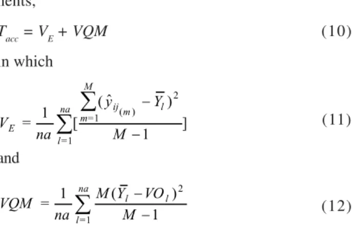
Tacc = VE + VQM (10)
in which
] 1
) ˆ
( [ 1 =
2 ) ( 1 =
1
=
-å
å
M Y y
na V
l m ij M
m na
l
E (11)
and
1 ) (
1 =
2
1
=
-å
M YM VOna
VQM l l
na
l
(12)
The first component (VE) represents the pooled variance between imputations within positions, there-fore the greater its value is, the smaller is the preci-sion of the multiple imputation method. However, a small value for this component does not necessarily mean that the imputation method is good, for the method may be biased. The second component (VQM) represents the average squared bias between the val-ues of and VO, so the smaller the bias is, the big-ger is the number of imputations that are similar to the original values and the greater is their accuracy. There-fore, the smaller are the values of VE and VQM, the larger is the multiple imputation method.
RESULTS AND DISCUSSION
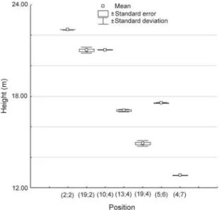
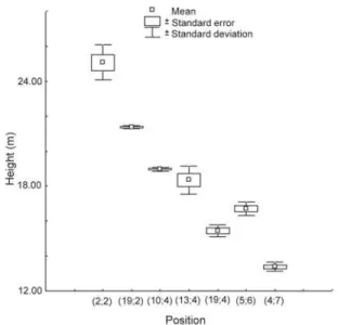
Table 1 gives the results for 5%, 10% and 30% of missing values of a random deletion in the matrix. The variability between imputations within each miss-ing value is relatively small, as shown by the small co-efficients of variation. Furthermore, this variability in-creases as the percentage of missing data rises from 5% to 10%, except at the position (19;2) (Figures 1 and 2). When the percentage of missing values in-creases from 10% to 30%, the variability inin-creases at positions (19;2), (10;4) and (19;4), and it decreases at positions (2;2), (13;4), (5;6) and (4;7) (Figures 2 and 3). The overall precision of multiple imputation is good for these data (Tables 1-2). As for the accuracy, which is the difference between the imputed values and the original values, this shows less consistency than the precision. Values of acc are nearly all larger than their counterparts Var in Table 1, but the pattern is more variable in the other table. So there is no clear relationship between precision and accuracy over the individual missing value positions.
percent-Table 1 - Imputations for mean heights (m) at each position (ith row; jth column) of a random deletion (5%, 10% and 30%
missing).
VO: Original value. : Imputations means. Var: Variance between imputations. CV : Coefficient of variation. acc : Accuracy. n
o i t e l e D
n o i t i s o
p VO
n o i t a t u p m I
1 2 3 4 5 Var CV acc
g n i s s i m % 5
) 2 ; 2
( 24.00 22.37 22.35 22.35 22.35 22.35 22.35 0.0001 0.04 3.380
) 2 ; 9 1
( 20.12 21.37 20.93 20.93 20.93 20.93 21.02 0.0387 0.94 1.051
) 4 ; 0 1
( 18.94 21.06 21.05 21.03 21.02 21.01 21.03 0.0004 0.10 5.469
) 4 ; 3 1
( 18.78 16.90 17.08 17.09 17.10 17.11 17.06 0.0077 0.52 3.724
) 4 ; 9 1
( 15.68 14.58 14.97 14.98 15.00 15.01 14.91 0.0339 1.23 0.776
) 6 ; 5
( 18.06 17.50 17.58 17.57 17.55 17.54 17.55 0.0010 0.18 0.327
) 7 ; 4
( 13.03 12.82 12.80 12.80 12.80 12.81 12.81 0.0001 0.07 0.064
g n i s s i m % 0 1
) 2 ; 2
( 24.00 23.30 25.62 25.13 25.65 25.64 25.07 1.0263 4.04 2.454
) 2 ; 9 1
( 20.12 21.53 21.33 21.26 21.40 21.33 21.37 0.0101 0.48 1.925
) 4 ; 0 1
( 18.94 18.85 18.92 18.90 19.06 19.06 18.96 0.0097 0.51 0.010
) 4 ; 3 1
( 18.78 16.88 18.71 18.67 18.74 18.73 18.35 0.6723 4.47 0.908
) 4 ; 9 1
( 15.68 14.82 15.53 15.55 15.68 15.68 15.45 0.1306 2.33 0.197
) 6 ; 5
( 18.06 16.78 16.03 16.92 16.89 16.89 16.70 0.1425 2.27 2.445
) 7 ; 4
( 13.03 12.92 13.52 13.56 13.46 13.45 13.38 0.0703 1.96 0.226
g n i s s i m % 0 3
) 2 ; 2
( 24.00 23.78 23.94 23.14 23.22 22.94 23.40 0.1855 1.85 0.630
) 2 ; 9 1
( 20.12 21.60 21.62 21.88 21.88 21.90 21.78 0.0226 0.70 3.441
) 4 ; 0 1
( 18.94 19.00 19.78 18.86 18.72 18.98 19.07 0.1725 2.17 0.193
) 4 ; 3 1
( 18.78 16.43 16.33 17.05 15.93 16.27 16.40 0.1666 2.49 7.219
) 4 ; 9 1
( 15.68 15.11 14.57 15.46 14.22 15.69 15.01 0.3703 4.07 0.932
) 6 ; 5
( 18.06 17.64 17.17 17.59 17.67 17.67 17.55 0.0458 1.22 0.375
) 7 ; 4
( 13.03 12.63 12.73 12.61 12.72 12.71 12.68 0.0030 0.44 0.155 Y
Table 2 - General performance measure of the proposed multiple imputation method, with 5%, 10% and 30% missing values.
y c a r u c c a l a r e n e G
g n i s s i
M VE VQM Tacc
%
5 0.0119 2.1012 2.1131
% 0
1 0.1700 1.2831 1.4531
% 0
3 0.2070 1.2011 1.4081
Figure 1 - Mean imputation height, standard error and standard deviation with 5% missing values.
age of missing values rises, the variation between im-putations defined by expression (11) increases while the average squared bias defined by expression (12) decreases. This results in an improvement of the overall performance, which can be seen through the decrease in the general measure as defined by expression (10).
assump-Figure 2 - Mean imputation height, standard error and standard deviation with 10% missing values, for the same positions as the data with 5% missing values.
Figure 3 - Mean imputation height, standard error and standard deviation with 30% missing values, for the same positions as the data with 5% missing values.
tions about the distribution or structure of the data. In the G × E interaction matrix for the E. grandis height data, the variability in relation to the mean of imputed values is small, indicating a high precision, and the bias in relation to the original values is also small, indicating good accuracy. However, its values are greater than the variability in relation to the imputed values mean, indicating less accuracy in the proposed model.
ACKNOWLEDGMENTS
To CAPES and CNPq for the award of a scholarship to G.C. Bergamo and C.T.S. Dias, respec-tively.
REFERENCES
GOOD, I.J. Some applications of the singular value decomposition of a matrix Technometrics, v.11, p.823-831, 1969. KRZANOWSKI, W.J. Cross-validation in principal component
analysis. Biometrics, v.43, p.575-584, 1987.
KRZANOWSKI, W.J. Missing value imputation in multivariate data using the singular value decomposition of a matrix.
Biometrical Letters, v.25, p.31-39, 1988.
LAVORANTI, O.J. Estabilidade e adaptabilidade fenotípica através da reamostragem “bootstrap” no modelo AMMI. Piracicaba: USP/ESALQ, 2003. 166p. Tese (Doutorado).
LITTLE, R.J.; RUBIN, D.B. Statistical analysis with missing
data. 2nd
ed. New York: John Wiley, 1987. 278p.
LITTLE, R.J.; RUBIN, D.B. Statistical analysis with missing data. New York: John Wiley, 2002. 381p.
MOLENBERGHS, G.; VERBEKE, G. Models for discrete
longitudinal data. New York: Springer Science, 2005. 683p. PENNY, K.I.; JOLLIFFE, I.T. Multivariate outlier detection applied to multiply imputed laboratory data. Statistics in Medicine, v.18, p.1879-1895, 1999.
RUBIN, D.B. Multiple imputation in sample surveys: a phenomenological Bayesian approach to nonresponce. In: SURVEY RESEARCH METHODS SECTION OF THE AMERICAN STATISTICAL ASSOCIATION, 1978.
Proceedings. p.20-34. Available at: http://www.amstat.org/ sections/srms/Proceedings/. Accessed 20 Nov. 2006.
RUBIN, D.B. Multiple imputation for nonresponce in surveys. New York: John Wiley, 1987. 258p.
RUBIN, D.B.; SCHENKER, N. Multiple imputation for interval estimation from simple random samples with ignorable nonresponse. Journal of the American Statistical
Association, v.81, p.366-374, 1986.
SAS INSTITUTE. SAS/IML 9.1: user‘s guide. Carey: SAS Institute, 2004a. 1040p.
SAS INSTITUTE. SAS/STAT 9.1: user‘s guide. Carey: SAS Institute, 2004b. 5121p.
SCHAFER, J.L. Analysis of incomplete multivariate data. London: Chapman & Hall, 1997. 430p.
SCHAFER, J.L. Multiple imputation: a primer. Statistical Methods in Medical Research, v.8, p.3-15, 1999.
TANNER, M.A.; WONG, W.H. The calculation of posterior distributions by data augmentation (with discussion). Journal
of the American Statistical Association, v.82, p.528-550, 1987.
ZHANG, P. Multiple imputation: theory and method.
International Statistical Review, v.71, p.581-592, 2003. Received March 29, 2007