Missing value imputation in multi-environment
trials: Reconsidering the Krzanowski method
Sergio Arciniegas-Alarcón
1*, Marisol García-Peña
1and Wojtek
Krzanowski
2Abstract:We propose a new methodology for multiple imputation when faced
with missing data in multi-environmental trials with genotype-by-environment interaction, based on the imputation system developed by Krzanowski that uses the singular value decomposition (SVD) of a matrix. Several different iterative variants are described; differential weights can also be included in each variant to represent the influence of different components of SVD in the imputation process.The methods are compared through a simulation study based on three real data matrices that have values deleted randomly at different percentages, using as measure of overall accuracy a combination of the variance between imputations and their mean square deviations relative to the deleted values. The best results are shown by two of the iterative schemes that use weights belonging to the interval [0.75, 1]. These schemes provide imputations that have higher quality when compared with other multiple imputation methods based on the Krzanowski method.
Key words: Singular value decomposition, weights, missing data,
genotype-by-environment interaction, plant breeding.
Crop Breeding and Applied Biotechnology 16: 77-85, 2016 Brazilian Society of Plant Breeding. Printed in Brazil
http://dx.doi.org/10.1590/1984-70332016v16n2a13
ARTICLE
*Corresponding author:
E-mail: [email protected]
Received: 06 November 2014 Accepted: 15 December 2015
1 Universidade de São Paulo/ESALQ,
Departa-mento de Ciências Exatas, C.P. 09, 13.418-900, Piracicaba, SP, Brazil.
2 University of Exeter, College of Engineering,
Mathematics and Physical Sciences, Harrison Building, North Park Road, Exeter, EX4 4QF, United Kingdom INTRODUCTION
In plant breeding, multi-environment trials are important in order to test the general and specific adaptation of cultivars. A cultivar which grows in different environments will show significant fluctuations of performance in production relative to other cultivars. These changes are influenced by different environmental conditions; and in crop science literature they are commonly referred to as genotype-by-environment interactions, or G×E. Some useful
references can be found in Arciniegas-Alarcón et al. (2013).
Although G×E trials are planned to be balanced, missing values occur for
various reasons, such as removal of underperforming genotypes, inclusion of new genotypes, human errors or natural causes. For instance, plants might be destroyed by animals, by floods, or during the harvest, while yield measurements may be erroneously carried out or incorrectly entered into the data base (Rodrigues et al. 2011).
values (Gabriel 2002, Arciniegas-Alarcón et al. 2014a).
Possible ways of analysing G×E trials containing missing values are: i) extracting a balanced subset of data, by deleting
those genotypes or environments which contain any missing values (Ceccarelli et al. 2007, Yan et al. 2011); ii) filling the missing cells with environmental means; or iii) filling the missing cells with values estimated from fitted multiplicative or mixed linear models (Arciniegas-Alarcón et al. 2011, Kumar et al. 2012). Some researchers prefer to use either the mixed linear model based on the statistical method of Restricted Maximum Likelihood/Best Linear Unbiased Prediction (REML/BLUP) or Bayesian approaches. For a description of these methodologies see, e.g., Fritsche-Neto et al. (2010), Crossa et al. (2011), Josse et al. (2014) and Omer et al. (2015).
These strategies may overcome the lack of balance in the data, but none of them is simple and effective (Yan 2013). The first strategy does not make use of all the available information; the second one may have problems when too many values are missing; and the third one involves multiple steps and complicated procedures. See Yan (2013) for details.
Krzanowski (1988) proposed a perfectly general imputation scheme free of any distributional and structural constraints, which uses SVD to impute missing values. The scheme can be used on any data set that can be arranged in matrix form and, therefore, can be applied in G×E trials. The procedure provides simple imputation; however, Josse
and Husson (2012) and van Buuren (2012) have warned that such methods do not take into account the uncertainty produced by the imputation. Moreover, if parameters are subsequently estimated from the imputed values, then the standard errors will be underestimated, which means that confidence intervals and tests will not be valid, even if the imputation model is correct.
In order to solve this problem, multiple imputation (MI) (Rubin 1987, Harel and Zhou 2007, Allison 2012, Rässler et al. 2013) can be used. This involves three distinct steps: i) Imputation: The missing values are estimated M times,
generating M completed data sets (observed+imputed); ii) Analysis: The M completed data sets are analyzed using
appropriate statistical procedures for the problem at hand; iii) Combination: The M separate sets of results are combined
into one single inference.
The literature and the associated statistical software provide several alternatives of MI, such as the parametric regression, the propensity score method, or the Markov chain Monte Carlo (MCMC) method (Zhang 2003, Yuan 2011). However, these methodologies require that certain assumptions are met. The assumption in all three methods is that the missing data depend on observed variables, which means that there is a missing at random mechanism (MAR), as defined by Little and Rubin (2002). Also, parametric regression and MCMC depend on the assumption of multivariate normality.
In this paper, a method is proposed for the first step of MI that does not make any distributional or structural assumptions in G×E experiments, by modifying the algorithm presented by Krzanowski (1988), and taking related
literature into account.
MATERIAL AND METHODS
In order to describe the Krzanowski method, consider a matrix Y (n×p) with elements y
ij (i = 1,...n; j=1...p) and n
> p (if n < p, the matrix should be first transposed). First, suppose there is just one missing value yij in Y. Then, delete
the i-th row from Yand calculate the SVD for the ((n – 1)×p) resulting matrix Y(–i) as Y(–i) = U D VT, U =(u
sh), V =(vsh), D =
(d1,...,dp). For the next step, delete the j-th column from Y in order to obtain the SVD for the (n×(p – 1)) matrix Y
(–j) as Y(–j)
= ~U~D~VT, ~U =(~ush), ~V =(~vsh) , ~D = (~d1,...,~dp–1) . The matrices U, V, ~U and ~V are orthonormal, while ~D and D are diagonal.
Afterwards, combine the two SVDs, Y(–i) and Y
(–j), and the imputed value will be given by
(
)
(
)
∑
=
= H
h
h jh h ih
ij u d v d
y 1
~ ~
ˆ (1)
whereH = min{n – 1, p – 1}. When there is more than one missing value, an iterative scheme is required as follows.
Initially replace all missing values by their respective column means, giving a completed matrix Y, and then standardize
the columns by subtracting mj and dividing the result by sj (where mj and sj represent the mean and the standard
deviation of the j-th column calculated only from the observed values). Using the standardized matrix, recalculate the
imputation for each missing value using the equation (1). Finally, return the matrix Yto its original scale, yij = mj + sjyˆij. Then iterate the process until stability is achieved in the imputations. In order to avoid convergence problems, a parity check should be done in each iteration by matching the sign of
(
u
~
ihd
~
h)
(
v
jhd
h)
in (1) to the sign of uihdhvjh obtained
from the SVD of the Ymatrix for each h = 1,...,H(Eastment and Krzanowski 1982).
It is possible to avoid the parity check by using an alternative expression for (1) following the results of Bro et al. (2008). The authors suggest updating the missing yij by the corresponding element of the matrix
S = (~U(~U)+)Y(V(V)+)T (2)
where (•)+ represents the Moore-Penrose generalized inverse. It is noted that for each missing observation a different
S matrix will be calculated; the inclusion of (2) in the algorithm makes the imputation be basically an expectation
maximization (EM) operation (Bro et al. 2008).
On the other hand, to obtain MI from the Krzanowski method, Bergamo et al. (2008) proposed a generalization to the exponents of ~dh and dh, replacing equation (1) by
(
)
(
)
∑
= −=
H h a h jh a h ihij
u
d
v
d
y
1
1
~
~
ˆ
(3)wherea is the weight in the interval [0,1] given to Y
(–j). Specification of a automatically determines the weight for Y(–i). For example, a weight a=0.4 for Y
(–j) gives the weight 1-a=0.6 for Y(–i). Bergamo et al. (2008) assert that 5 imputations for each missing value is enough to ensure variability among imputations. For this reason, the authors suggest using weights a=0.4, 0.45. 0.50, 0.55 and 0.60 in turn for Y
(–j), each value of a providing a different imputation.
Recently, Arciniegas-Alarcón et al. (2014b) have used a small modification for equation (3). They included two constants to eliminate the bias produced by the systematic underestimation of ~D and D in relation to D (Louwerse et
al. 1999), using the expression
(
)
(
)
(
(
)
)
∑
= −−
−
=
H h a h jh a h ihij
u
d
p
p
v
d
n
n
y
1 11
1
~
~
ˆ
(4)In (4), the number of components H needs first to be specified. Krzanowski (1988) and Bergamo et al. (2008) used H = min{n–1, p–1} with the objective of using the maximum available information in the matrix. However, this choice
can produce low efficiency of imputation in multi-environment trials (Arciniegas-Alarcón and Dias 2009) and lead to convergence problems (Hedderley and Wakeling 1995). For these reasons, the authors obtained better results by choosing H = min{A,B}, where A is such that
{ } 7 5 . 0 1 , 1 min 1 2 1 2 ≈
∑
∑
− − = = p n h h A h h dd and B is such that
{ }
75 . 0 ~ ~ min 1, 1
1 2 1 2 ≈
∑
∑
− − = = p n h h B h h d d .To propose an alternative methodology of MI based on the Krzanowski method, it is suggested that a multiplicative weight wt ϵ [0,1] is included in equation (1). Thus the following expression is used:
(
)
(
)
∑
= = H h h jh h ih tij w u d v d
y 1
~ ~
ˆ (5)
with t=1,...,M , where M represents the number of imputations, so that the inclusion of different weights will produce
different imputations for each missing value. Again, M=5 can be used, since this number produces good statistical
efficiency in many practical applications (van Buuren 2012). Each weight wt can be interpreted as the influence placed
on the SVD components in the final imputation, similar to that in the iterative scheme using mj + sjyˆij. For instance, if the weight wt is low, the imputation will depend more on the column means, which are updated in each iteration. Similarly,
the weight wt can also be included in equation (2) to obtain another MI form S
t = wt(
~
U(~U)+)Y(V(V)+)T (6)
The influence of the SVD in the imputation was defined in terms of percentage. Thus, the interval between 0 and 1 was used for wt, and seven groups of values were considered: Group1 = 0, 0.05, 0.1, 0.15, 0.2; Group2 = 0.25, 0.3, 0.35,
0.4, 0.45; Group3 = 0.5, 0.55, 0.60, 0.65, 0.7; Group4 = 0.75, 0.8, 0.85, 0.9, 0.95; Group5 = 0.96, 0.97, 0.98, 0.99, 1; Group 6: 0.2, 0.4, 0.6, 0.8, 1; and Group7 contains 5 random numbers from the uniform distribution, i.e.,wt ~U[0,1]. The groups
ih
ij
ij
ij ih jh
jh ih
ih jh
jh
were empirically defined following the work of Arciniegas-Alarcón et al. (2014a), which proposed MI in incomplete two-way tables through a variation in the exponents of the diagonal matrix elements obtained in the calculation of a SVD. With the seven groups for wt, and the two new proposed equations for imputation, there are in total 14 possible
variations of MI under the Krzanowski system. These variations are denoted “SVDi+PC” and “SVDi+EM”, with i =1,...,7. Here, “SVDi+PC” indicates the iterative scheme with parity check using equation (5) and group i for the values of w
t, while
“SVDi+EM” indicates the iterative scheme with EM imputation using the equation (6) and group i for the values of w t.
These 14 variations were assessed against the iterative scheme with parity check that uses equation (4) for imputation. This latter method was treated as the standard method (or “gold standard”), and was denoted “MIK-Adjusted”. An extension of “MIK-Adjusted” was also included by assuming that the exponent a can be chosen randomly, and a~U[0,1];
this extension was called “Unif-MIK-Adjusted”. Both “MIK-Adjusted” versions and the variations described above need the value of H (i.e. the number of components of SVD to be retained) to be previously determined. This value was obtained
using the cv.SVDImpute function of the imputation package from R, which carries out cross-validation in incomplete matrices (Wong 2013, García-Peña et al. 2014, Arciniegas-Alarcón et al. 2014b).
To evaluate the imputation systems, the methodology proposed by Yan (2013) was used, by taking complete real multi-environmental matrices, randomly deleting observations from them at different percentages, applying the algorithms, and then using appropriate summary statistics to compare the imputations with the real data. Molale et al. (2013) describe some of these performance measures, such as: the Root Mean Square Error (RMSE), the Mean Absolute Error (MAE), the Relative Absolute Error (RAE), and the Root Relative Squared Error (RRSE). These statistics serve to evaluate any imputation system; however, to assess new MI methods, it would be more appropriate to use statistics involving the variability between imputations. For this, Penny and Jolliffe (1999) introduced the Tacc statistics, which will be used in this study and which is described below.
Three data sets from G×E trials were considered, which had been previously used by Lavoranti et al. (2007), Yang
(2007) and Rad et al. (2013), respectively. The first data set (Rad et al. 2013) consists of a 36×6 matrix for 36 wheat
genotypes assessed in six environments under normal and drought stress conditions, at an experimental farm of the University of Putra, Malaysia. The studied variable was the mean plant grain yield (gr). The second data set (Lavoranti et al. 2007) comprises a 20×7 matrix, for 20 Eucalyptus grandis progenies assessed in seven locations in the south and
southeast regions of Brazil, and the studied variable was mean tree height (m). Lastly, the third data set (Yang 2007)
is a 6×18 matrix, corresponding to six barley genotypes assessed in 18 environments in Alberta, Canada. The studied
variable was yield (Mg ha-1).
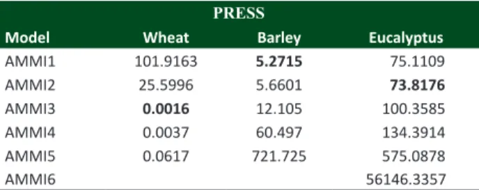
Table 1 shows the results from a preliminary study on the choice of the number of multiplicative components (to explain the G×E interaction) of the AMMI model that can be used for each selected data set, on which a simulation study is described below. The method of cross-validation “leave-one-out” by eigenvector (Bro et al. 2008, Gauch 2013) was used to select each model, and the best model was the one which has the lowest PRESS statistics. It can be seen that AMMI3 is an appropriate model for the wheat matrix; AMMI1 is appropriate for the barley matrix; and AMMI2 is appropriate for the eucalyptus matrix. Therefore, these three data sets represent a wide range of data sizes and structures typically found in G×E trials, and thus provide good basis for drawing general conclusions for such trials.
Each original data matrix (wheat, eucalyptus and barley) was submitted to random deletion of values at the three rates 10%, 20%, and 35%, since according to Yan (2013), in G×E trials, generally, the number of missing values is
lower that 40%. The process was repeated in each data set replicated 1000 times for each percentage of missing values, giving a total of 3000 different matrices with missing values. Altogether, therefore, 9000 incomplete data sets were available, and for each one, the missing values were imputed with the 16 MI algorithms, using computational code in R (R Core Team 2014).
Table 1.Values of Predicted REsidual Sum of Squares (PRESS)
us-ing cross validation by eigenvector in choosus-ing the AMMI model to explain the interaction in the original (complete) data matrices
PRESS
Model Wheat Barley Eucalyptus
AMMI1 101.9163 5.2715 75.1109
AMMI2 25.5996 5.6601 73.8176
AMMI3 0.0016 12.105 100.3585
AMMI4 0.0037 60.497 134.3914 AMMI5 0.0617 721.725 575.0878
The random deletion process for a matrix Y(n×p) was carried out as follows. Random numbers between 0 and 1 were
generated in the R software with the runif function. For a fixed r value (0< r <1), if the (pi + j)-th random number was
lower than r, then the element in the (i+1, j) position of the matrix was deleted (i =0,1,...,n–1; j =1,...,p). The expected
proportion of missing values in the matrix will be r (Krzanowski 1988, Arciniegas-Alarcón et al. 2013). This technique
was used with r = 0.1, 0.2 and 0.35.
The imputation accuracy was assessed with the Tacc statistics, proposed by Penny and Jolliffe (1999), which has been recently used by Bergamo et al. (2008) and Arciniegas-Alarcón et al. (2014a). Tacc is a measure of overall accuracy formed from the sum of the pooled variance between imputation within positions (VE) and the mean squared bias between the imputations mean and the original value deleted in the simulation study (VQM). Thus: Tacc = V
E+VQM,
where ( )
(
)
∑
∑
= =
− − = na
l M
m
l m ij
E
M Y y
n a V
1 1
2
1 ˆ 1
and
∑
(
)
= −
− = na
l
l l
M VO Y M n a VQM
1
2
1 1
; in which “na” is the total number of
deleted values from the G×E matrix. Each deleted value l has the corresponding position (i, j) in the matrix, that is, in
the i-th row and the j-th column. Mis the number of imputations for the missing value l; yˆij(m) is the m-th imputation for
that value according to the proposed methods; Y
l is the imputations mean produced for the missing value l; and VOlis
the original value l in the complete original data set.
According to Penny and Jolliffe (1999), a good MI method will be that with small values for VE and VQM, which implies
low values of Tacc. Thus, since “MIK-Adjusted” was treated as the standard method,any method having values for Tacc lower than those for “MIK-Adjusted” was considered as a good imputation method. It is worth pointing out that only having a reduced value of VE does not imply good imputation quality, since the method can be biased.
RESULTS
Wheat data
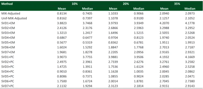
Table 2 shows the means and medians of Tacc, at the different percentages of values deleted randomly (10, 20 and 35%) for the wheat data set. The best results at each imputation percentage (minimizing the mean and median of Tacc) were obtained by SVD4+EM and SVD5+EM. At 35% imputation, SVD4+PC and SVD5+PC were also better than any of the MIK methods. These results indicate that the weights of wt should be chosen in the interval [0.75;1]. However, the values
Table 2.Means and medians of T
acc at different percentage levels for the wheat data
Method 10% 20% 35%
Mean Median Mean Median Mean Median
MIK-Adjusted 0.8134 0.7405 1.1033 0.9066 2.0940 2.0973
Unif-MIK-Adjusted 0.8162 0.7397 1.1078 0.9100 2.1257 2.1052
SVD1+EM 3.8823 3.7468 3.9793 3.9349 4.2070 4.1778
SVD2+EM 2.4126 2.3176 2.6866 2.5963 3.2988 3.2952
SVD3+EM 1.3213 1.2417 1.6496 1.5215 2.5055 2.5268
SVD4+EM 0.6867 0.6477 0.9704 0.8123 1.9740 2.0524
SVD5+EM 0.5677 0.5319 0.8362 0.6781 1.9511 1.9913
SVD6+EM 1.6024 1.5292 1.8847 1.7768 2.7013 2.7187
SVD7+EM 1.9681 1.8278 2.2205 2.0956 2.9165 2.9321
SVD1+PC 3.9073 3.7755 3.9881 3.9506 4.1932 4.1669
SVD2+PC 2.4975 2.3961 2.7339 2.6276 3.2761 3.2582
SVD3+PC 1.4725 1.3911 1.7536 1.6124 2.4960 2.5258
SVD4+PC 0.9010 0.8361 1.1628 1.0035 2.0045 2.0862
SVD5+PC 0.8086 0.7371 1.0855 0.9024 2.0285 2.0471
SVD6+PC 1.7500 1.6724 2.0014 1.8781 2.7045 2.7380
SVD7+PC 2.1132 1.9294 2.3123 2.1814 2.9151 2.9143
na na
of Tacc in all the remaining 11 imputation systems were higher than for MIK-Adjusted. Therefore, the least recommended algorithms are those with w
t in the interval [0;0.45], namely SVDi+PC and SVDi+EM, with i=1,2.
The algorithms that assumed a uniform distribution for a in the case of Unif-MIK-Adjusted; for w
t, in the case of
SVD7+EM and SVD7+PC deserve special comment. The mean and the median values of Unif-MIK-Adjusted are very close to those of MIK-Adjusted, but never lower, and as the percentage of imputation increases, differences remained the same or even increased. The performances of SVD3+EM and SVD3+PC are better than those of SVD7+EM and SVD7+PC at all the percentages, which means that the insertion of a random component did not improve the imputation efficiency. One of the initial intentions of the simulation study for wheat data was to determine a set of algorithms that were better than MIK-Ajusted, and this is clearly achieved by SVD4+EM, SVD5+EM, SVD4+PC and SVD5+PC. Thus, the results will be considered consistent if at least one of the four imputation systems minimizes Tacc in the other multi-environmental data matrices.
Eucalyptus data
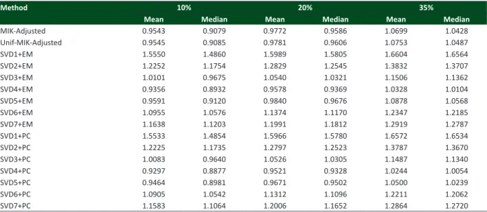
Table 3 shows the means and medians of Tacc, at the different percentages of values deleted randomly (10, 20 and 35%) for the eucalyptus data set. Similar behaviour was found to that described in the wheat data. For instance, i) Unif-MIK-Adjusted never beats the gold standard MIK-Adjusted, ii) SVD3+EM and SVD3+PC always perform better than SVD7+EM and SVD7+PC, respectively, and iii) the least recommended systems are SVDi+PC and SVDi+EM, with i=1,2, (i.e., the imputations less influenced by SVD due to the chosen weight), since they have the worst performance among the proposed methodologies.
SVD4+PC, SVD5+PC and SVD4+EM beat MIK-Adjusted in all the imputation percentages. It is worth mentioning that the means and medians of Tacc for SVD4+PC are lower than those of SVD4+EM, i.e., a method that involves a parity check beats an imputation of type EM – which is a different result from those found in wheat data. While in the wheat matrix SVD5+EM was better than MIK-Adjusted, here the opposite occurs.
Barley data
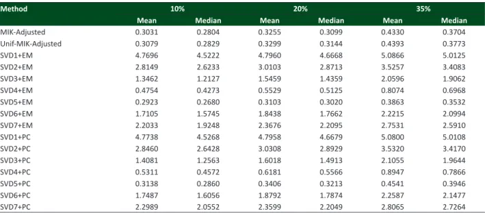
Table 4 shows the means and medians of Tacc, at the different percentages of values deleted randomly (10, 20 and 35%) for the barley data set. In this case, only SVD5+EM presents better results than MIK-Adjusted, while SVD4+EM, SVD4+PC and SVD5+PC exhibit higher values of Tacc than for the standard algorithm. The other 11 variations of the Krzanowski method presented the same behaviour of the wheat and eucalyptus data.
Table 3.Means and medians of T
acc at different percentage levels for the eucalyptus data
Method 10% 20% 35%
Mean Median Mean Median Mean Median
MIK-Adjusted 0.9543 0.9079 0.9772 0.9586 1.0699 1.0428
Unif-MIK-Adjusted 0.9545 0.9085 0.9781 0.9606 1.0753 1.0487
SVD1+EM 1.5550 1.4860 1.5989 1.5805 1.6604 1.6564
SVD2+EM 1.2252 1.1754 1.2829 1.2545 1.3832 1.3707
SVD3+EM 1.0101 0.9675 1.0540 1.0321 1.1506 1.1362
SVD4+EM 0.9356 0.8932 0.9578 0.9369 1.0328 1.0104
SVD5+EM 0.9591 0.9120 0.9840 0.9676 1.0878 1.0568
SVD6+EM 1.0955 1.0576 1.1374 1.1170 1.2347 1.2185
SVD7+EM 1.1638 1.1203 1.1991 1.1812 1.2919 1.2787
SVD1+PC 1.5533 1.4854 1.5966 1.5780 1.6572 1.6534
SVD2+PC 1.2225 1.1735 1.2797 1.2523 1.3787 1.3670
SVD3+PC 1.0083 0.9640 1.0526 1.0305 1.1487 1.1340
SVD4+PC 0.9297 0.8877 0.9521 0.9328 1.0244 1.0054
SVD5+PC 0.9464 0.8981 0.9671 0.9502 1.0500 1.0239
SVD6+PC 1.0905 1.0542 1.1312 1.1096 1.2211 1.2062
DISCUSSION
The main conclusion is that the MI methods which have been derived from the simple imputation system of Krzanowski may have advantages over the current standard method for a wide range of G×E interaction structures encountered
in practice. The four imputation systems SVDi+PC and SVDi+EM with i=4,5 showed better results than the standard method in simulations involving the largest matrix (216 observations), having the most complex interaction structure. For smaller matrices and less complex interactions, a subset of these four methods beat the standard. For the matrix with 140 observations and intermediate interaction structure, this subset comprised SVDi+PC and SVDj+EM for i=4,5 and j=4, while for the smallest matrix of 108 observations and simplest interaction structure, it contained just SVD5+EM.
In the light of these results, it is clear that it is only worthwhile considering weights w in the range [0.75, 1.0] (since
low values of w mean that the benefits of SVD are being ignored). However, some selection must be initially carried
out between the four sets of weights and the methods identified above as the best ones. A fast path in a practical case would be to test the set of four algorithms in order to determine the best one. However, a deeper analysis of the previous results should take into consideration the fact that each method has two parts: one related to the weight wt,
and the other related to the iterative scheme used (i.e. iterations with parity check or of type EM). According to Tacc, the best result is obtained when wt belongs to group 5 in the three considered matrices, as this always outperforms
MIK-Adjusted. On the other hand, a definitive conclusion about the iterative scheme could not be obtained. Thus, in a real situation of incomplete G×E matrices, it is recommended to test both systems SVD5+PC and SVD5+EM.
It is also worth commenting that in the context of cross-validation for components, Bro et al. (2008) pointed out that the Eastment and Krzanowski (EK) method (1982) has a problem of rotational freedom, and the parity check is a source of overfitting. However, in this study, it was found that, in some cases, the parity check within an iterative scheme can offer better predictions than the EM algorithm described by Bro et al. (2008). Thus a hypothesis to investigate in the future is that the influence of rotation problems and overfitting on the predictions might be minimized if EK is used iteratively.
Finally, the researcher may be interested in how to test SVD5+PC and SVD5+EM on a set of incomplete data. It is suggested that, starting with the observed data, some of the entries are randomly deleted (for instance, between 10% and 30%), the two algorithms are applied, and the Tacc statistic values are calculated. The deletion procedure is then repeated (for example, 100 times), and the mean and median of all the values are found. The method with the lowest mean or median will be the method to be used on the matrix with missing values. Another option is to choose the method according to the magnitude of the imputation uncertainty, using for the estimation the non-parametric methodology proposed by Heydarbeygie and Ahmadi (2013).
Table 4.Means and medians of T
acc at different percentage levels for the barley data
Method 10% 20% 35%
Mean Median Mean Median Mean Median
MIK-Adjusted 0.3031 0.2804 0.3255 0.3099 0.4330 0.3704
Unif-MIK-Adjusted 0.3079 0.2829 0.3299 0.3144 0.4393 0.3773
SVD1+EM 4.7696 4.5222 4.7960 4.6668 5.0866 5.0125
SVD2+EM 2.8149 2.6233 3.0103 2.8713 3.5257 3.4083
SVD3+EM 1.3462 1.2127 1.5459 1.4359 2.0596 1.9062
SVD4+EM 0.4754 0.4273 0.5529 0.5125 0.8074 0.6968
SVD5+EM 0.2923 0.2680 0.3103 0.3020 0.3863 0.3532
SVD6+EM 1.7105 1.5745 1.8438 1.7662 2.2215 2.0994
SVD7+EM 2.2033 1.9248 2.3676 2.2095 2.7531 2.5910
SVD1+PC 4.7738 4.5268 4.7958 4.6679 5.0800 5.0108
SVD2+PC 2.8460 2.6428 3.0308 2.8929 3.5320 3.4170
SVD3+PC 1.4081 1.2563 1.6018 1.4913 2.1055 1.9644
SVD4+PC 0.5311 0.4572 0.6181 0.5566 0.8947 0.7866
SVD5+PC 0.3138 0.2860 0.3406 0.3213 0.4541 0.3946
SVD6+PC 1.7487 1.6056 1.8792 1.7874 2.2587 2.1477
ACKNOWLEDGEMENTS
The first author thanks the Coordenação de Aperfeiçoamento de Pessoal de Nível Superior, CAPES, Brazil, (PEC-PG program) for the financial support. The second author thanks the National Council of Technological and Scientific Development, CNPq, Brazil, and the Academy of Sciences for the Developing World, TWAS, Italy, (CNPq-TWAS program) for the financial support.
REFERENCES
Allison PD (2012) Handling missing data by maximum likelihood. SAS Global Forum, Statistics and Data Analysis, 21p. (Paper 312).
Available at < http://www.statisticalhorizons.com/wp-content/ uploads/MissingDataByML.pdf > Accessed in May, 2016. Arciniegas-Alarcón S and Dias CTS (2009) Data imputation in trials with
genotype by environment interaction: an application on cotton data.
Biometric Brazilian Journal 27: 125-138.
Arciniegas-Alarcón S, Dias CTS and García-Peña M (2014a) Distribution-free multiple imputation in incomplete two-way tables. Pesquisa Agropecuária Brasileira49: 683-691.
Arciniegas-Alarcón S, García-Peña M and Dias CTS (2011) Data imputation in trials with genotype×environment interaction. Interciencia36:
444-449.
Arciniegas-Alarcón S, García-Peña M, Krzanowski WJ and Dias CTS (2013) Deterministic imputation in multienvironment trials. ISRN Agronomy 2013: 1-17.
Arciniegas-Alarcón S, García-Peña M, Krzanowski WJ and Dias CTS (2014b) Imputing missing values in multi-environment trials using the singular value decomposition: An empirical comparison. Communications in
Biometry and Crop Science 9:54-70.
Bergamo GC, Dias CTS and Krzanowski WJ (2008) Distribution free-multiple imputation in an interaction matrix through singular value decomposition. Scientia Agricola65: 422-427.
Bro R, Kjeldahl K, Smilde AK and Kiers HAL (2008) Cross-validation of component models: a critical look at current methods. Analytical
and Bioanalytical Chemistry 390: 1241-1251.
Ceccarelli S, Grando S and Baum M (2007) Participatory plant breeding in
water-limited environments. Experimental Agriculture 43: 411-435.
Crossa J, Perez-Elizalde S, Jarquin D, Cotes JM, Viele K, Liu G and Cornelius PL (2011) Bayesian estimation of the additive main effects and multiplicative interaction model. Crop Science 51: 1458-1469.
Eastment HT and Krzanowski WJ (1982) Cross-validatory choice of the number of components from a principal component analysis.
Technometrics24: 73-77.
Fritsche-Neto R, Gonçalves MC, Vencovsky R and Souza Junior CL (2010) Prediction of genotypic values of maize hybrids in unbalanced experiments. Crop Breeding and Applied Biotechnology 10: 32-39.
Gabriel KR (2002) Le biplot - outil d´exploration de données multidimensionelles. Journal de la Société Française de Statistique
143: 5-55.
García-Peña M, Arciniegas-Alarcón S and Barbin D (2014) Climate data imputation using the singular value decomposition: an empirical comparison. Revista Brasileira de Meteorologia29: 527-536.
Gauch H (2013) A simple protocol for AMMI analysis of yield trials. Crop Science53: 1860-1869.
Harel O and Zhou XH (2007) Multiple imputation: review of theory, implementation, and software. Statistics in Medicine26: 3057-3077.
Hedderley D and Wakeling I (1995) A comparison of imputation techniques for internal preference mapping, using Monte Carlo simulation. Food Quality and Preference 6: 281-297.
Heydarbeygie A and Ahmadi N (2013) Nonparametric methods for the estimation of imputation uncertainty. Journal of Applied Statistics
40: 693-698.
Josse J and Husson F (2012) Handling missing values in exploratory multivariate data analysis methods. Journal de la Société Française
de Statistique 153: 79-99.
Josse J, van Eeuwijk F, Piepho HP and Denis JB (2014) Another look at Bayesian analysis of AMMI models for genotype-environment data.
Journal of Agricultural, Biological, and Environmental Statistics
19: 240-257.
Krzanowski WJ (1988) Missing value imputation in multivariate data using the singular value decomposition of a matrix. Biometrical
Letters25: 31-39.
Kumar A, Verulkar SB, Mandal NP, Variar M, Shukla VD, Dwivedi JL, Singh BN, Singh ON, Swain P, Mall AK, Robin S, Chandrababu R,
Jain A, Haefele SM, Piepho HP and Raman A (2012) High-yielding,
drought-tolerant, stable rice genotypes for the shallow rainfed lowland droughtprone ecosystem. Field Crops Research133: 37-47.
Lavoranti OJ, Dias CTS and Krzanowski WJ (2007) Phenotypic stability and adaptability via AMMI model with bootstrap re-sampling. Pesquisa Florestal Brasileira 54: 45-52.
Little R and Rubin D (2002) Statistical analysis with missing data. 2nd edn,
John Wiley & Sons, New York, 408p.
Louwerse DJ, Smilde AK and Kiers HAL (1999) Cross-validation of multiway component models. Journal of Chemometrics 13: 491-510.
Penny KI and Jolliffe IT (1999) Multivariate outlier detection applied to multiply imputed laboratory data. Statistics in Medicine 18: 1879-1895.
R Core Team (2014) R: A language and environment for statistical
computing. R Foundation for Statistical Computing, Vienna. Available
at <http://www.R-project.org/.> Accessed in may 2014.
Rad MRN, Kadir MA, Rafii MY, Jaafar HZE, Naghavi MR and Ahmadi F (2013) Genotype × environment interaction by AMMI and GGE biplot analysis in three consecutive generations of wheat (Triticum aestivum) under normal and drought stress conditions. Australian Journal of Crop Science 7: 956-961.
Rässler S, Rubin DB and Zell ER (2013) Imputation. WIREs Computational
Statistics5: 20-29.
Rodrigues PC, Pereira DGS and Mexia JT (2011) A comparison between
joint regression analysis and the additive main and multiplicative interaction model: the robustness with increasing amounts of missing data. Scientia Agricola 68: 697-705.
Rubin DB (1987) Multiple imputation for nonresponse in surveys. John Wiley & Sons, New York, 258p.
van Buuren S (2012) Flexible imputation of missing data. CRC, Boca
Raton, 343p.
Wong J (2013) Imputation. Version 2.0.1. Available at: <http://CRAN. Rproject.org/package=imputation>. Accessed on October 15, 2013. Yan W (2013) Biplot analysis of incomplete two-way data. Crop Science
53: 48-57.
Yan W, Kang MS, Ma BL, Woods S and Cornelius PL (2007) GGE biplot
vs. AMMI analysis of genotype-by-environment data. Crop Science 47: 641-653.
Yan W, Pageau D, Frégeau-Reid J and Durand J (2011) Assessing the
representativeness and repeatability of test locations for genotype evaluation. Crop Science51: 1603-1610.
Yang RC (2007) Mixed-model analysis of crossover genotype–environment
interactions. Crop Science 47: 1051-1062.
Yang RC, Crossa J, Cornelius PL and Burgueño J (2009) Biplot analysis
of genotype × environment interaction: Proceed with caution. Crop Science 49: 1564-1576.
Yuan Y (2011) Multiple imputation using SAS software. Journal of
Statistical Software 45: 1-25.
Zhang P (2003) Multiple imputation: Theory and method. International