On the function of the floccular complex of the vertebrate cerebellum: implications in paleoneuroanatomy

On the function of the floccular complex of the vertebrate cerebellum:

implications in paleoneuroanatomy

Sérgio Filipe Ferreira Cardoso

Dissertação para obtenção do Grau de Mestre em Paleontologia

Orientador:

Doutor Rui Alexandre Ferreira Castanhinha

Co-orientadores:

Doutor Ricardo Miguel Nóbrega Araújo Prof. Doutor Miguel Telles Antunes

I

On the function of the floccular complex of the vertebrate cerebellum:

implications in paleoneuroanatomy

Sérgio Filipe Ferreira Cardoso

Dissertação para obtenção do Grau de Mestre em Paleontologia

Orientador:

Doutor Rui Alexandre Ferreira Castanhinha

Co-orientadores:

Doutor Ricardo Miguel Nóbrega Araújo Prof. Doutor Miguel Telles Antunes

Successfully defended on 18th November 2015 at FCT-UNL Campus, Portugal, before a juri presided over by:

Doutor Paulo Alexandre Rodrigues Roque Legoinha and consisting of:

Doutor Gabriel José Gonçalves Martins Doutor Rui Alexandre Ferreira Castanhinha

III

Direitos de autor - Copyright

Os direitos de autor deste documento pertencem a Sérgio Filipe Ferreira Cardoso, à FCT/UNL, à UNL e à UÉ. A Faculdade de Ciências e Tecnologia, a Universidade Nova de Lisboa e a Universidade de Évora têm o direito, perpétuo e sem limites geográficos, de arquivar e publicar esta dissertação através de exemplares impressos reproduzidos em papel ou de forma digital, ou por qualquer outro meio conhecido ou que venha a ser inventado, e de a divulgar através de repositórios científicos e de admitir a sua cópia e distribuição com objectivos educacionais ou de investigação, não comerciais, desde que seja dado crédito ao autor e editor.

Two peer-reviewed abstracts, resulting from this study, were accepted for oral communications (Appendix II).

Ferreira-Cardoso, S., Araújo, R., Castanhinha, R., Walsh, S., Martins, R.M.S., Martins, G.G. (2014). The Floccular Complex: neuroanatomy as a tool to unveil paleoecology. Journal of Vertebrate Paleontology, Program and Abstracts, 2014, p.128.

Ferreira-Cardoso, S., Castanhinha, R., Araújo, R., Walsh, S., Martins, N.E.V., Martins, R.M.S., Martins, G.G., Kardjilov, N., Hilger, A. (2015). Floccular Complex Lobe size does not correlate with vertebrate ecology and behavior. Journal of Vertebrate Paleontology, Program and Abstracts, 2015, p.123.

The latter was awarded with a Jackson School of Geosciences Student Member Travel Grant for the 2015 Society of Vertebrate Paleontology Annual Meeting.

At the moment, this study is in submission process to Scientific Reports journal, with the following list of authors: Sérgio Ferreira Cardoso, Ricardo Araújo, Stig Walsh, Nelson E. Martins, Gabriel G. Martins, Rui M.S. Martins, Nikolay Kardjilov, André Hilger, Ingo Manke and Rui Castanhinha.

I therefore request that this document is not made available for public consultation before the publishing process is completed.

IV

„Look I gotta go, yeah, I'm running outta change;

There's a lot of things if I could I'd rearrange‟.

Paul Hewson, David Evans, Adam Clayton & Lawrence Mullen, „The Fly‟, Achtung Baby.

V

Acknowledgments

I would like to thank my mother, Ana Ferreira, and father, Sérgio Cardoso, for supporting me in this adventure that is the study of evolution. I also want to thank the rest of my family, especially my sister, Jéssica, grandfather, Duarte and grandmother, Lourdes.

I would like to thank Rui Castanhinha and Ricardo Araújo for advising, guiding and helping me to understand science, the scientific world and, above everything else, the role of a scientist in the community. Their contribution for this study, in all its components, and for my improvement as a scientist and a person was essential.

I want to thank Professor Miguel Telles Antunes for his criticism and advices.

I would like to thank Professora Ausenda Balbino for her help and support.

I also want to thank: Nelson Martins (IGC), for his help with statistics; Gabriel Martins (IGC), for his contribution to solve 3D segmentation issues; Stig Walsh (National Museums Scotland), for sharing bird data and his ideas; Nikolay Kardjilov, André Hilger and Ingo Manke (HZB), for their essential contribution with mammal data scanning; Christiane Funk, for her help and availability to give me access to Museum für Naturkunde‟s mammal collections.

I would like to show my gratitude to Instituto Gulbenkian de Ciência, Helmholtz Zentrum Berlin, Museum für Naturkunde, Museu da Lourinhã and Digital Morphology Museum for allowing me to use their facilities, collections or data bases.

I want to thank Fundação para a Ciência e Tecnologia (FCT) for supporting this work through the project EXPL/BIA-EVF/0665/2013 (PALEOTECH).

Finally, I want to thank Zanildo Macungo, Albano Nhassengo and Nelson Nhamutole (Museu Nacional de Geologia) for making science and for letting me be part of their science and also Issaia Macaneta and all other people involved in the PalNiassa project for building a better world.

VII Abstract

The cerebellum floccular complex lobes (FCLs) are housed in the FCL fossa of the periotic complex. There is experimental evidence indicating that the FCLs integrate visual and vestibular information, responsible for the vestibulo-ocular reflex, vestibulo-collic reflex, smooth pursuit and gaze holding. Thus, the behavior of extinct animals has been correlated with FCLs dimension in multiple paleoneuroanatomy studies.

Here I analyzed braincase endocasts of a representative sample of Mammalia (48 species) and Aves (59 species) rendered using tomography and image segmentation and tested statistical correlations between the floccular complex volume, ecological and behavioral traits to assess various previously formulated paleobiological speculations.

My results demonstrate: 1) there is no significant correlation between relative FCL volume and body mass; 2) there is no significant correlation between relative FCL and optic lobes size in birds; 3) average relative FCL size is larger in diurnal than in nocturnal birds but there is no statistically significant difference in mammals; 4) feeding strategies are related with different FCL size patterns in birds, but not in mammals; 5) locomotion type is not related with relative FCL size in mammals; 6) agility is not significantly correlated with FCL size in mammals.

I conclude that, despite the apparent relation between FCL size and ecology in birds, the cerebellum of tetrapods is a highly plastic structure and may be adapted to control different functions across different taxonomic levels. For example, the european mole (Talpa europaea) which is fossorial and practically blind, has a FCL fossae relative size larger than those of bats, which are highly maneuverable. Therefore, variation in FCL size may be better explained by a combination of multiple factors with relation to anatomical and phylogenetic evolutionary constraints.

IX Resumo

Os lobos do complexo flocular (FCLs), alojados na fossa de FCL no complexo periótico, fazem parte do cerebelo. Existem provas experimentais da integração de informação visual e vestibular pelos FCLs, sendo responsáveis pelo reflexo vestibulo-ocular, vestibulo-cólico, pela manutenção do foco visual em objectos em movimento e pela estabilização da imagem. Assim, a dimensão dos FCLs e o comportamento de animais extintos têm sido associados em vários trabalhos sobre paleoneuroanatomia.

Analisei moldes da cavidade craniana de amostras representativas de mamíferos (48 espécies) e aves (59 espécies) produzidos a partir de tomografia e segmentação de imagens. Foram testadas correlações estatísticas entre volume do complexo flocular e variáveis ecológicas/comportamentais para investigar a veracidade das especulações paleobiológicas. Os dados foram analisados com recurso regressões linearres com correcção filogenética (PGLS). Os resultados mostram que: 1) não existe correlação entre volume relativo do FCL e massa corporal; 2) não existe correlação entre tamanho relativo do FCL e os lobos ópticos das aves; 3) a dimensão relativa de FCL é maior em aves diurnas que em aves nocturnas, não havendo significância estatística para os mamíferos; 4) as estratégias alimentares estão relacionadas com diferentes padrões dimensionais de FCL em aves, mas não em mamíferos; 5) o tipo de locomoção não está relacionado com o tamanho de FCL em mamíferos; 6) a agilidade não está correlacionada com a dimensão de FCL em mamíferos.

Conclui-se que, apesar da aparente relação entre dimensão de FCL e ecologia das aves, o cerebelo é uma estrutura altamente plástica, podendo sofrer adaptações para desempenhar funções distintas em diferentes grupos taxonómicos. Por exemplo, a toupeira europeia (Talpa europaea), que é fossorial e praticamente cega, tem fossas de FCL relativamente maiores que os morcegos, altamente manobráveis. Sendo assim, a variação da dimensão de FCL deverá estar relacionada com factores múltiplos, sejam eles ecológicos ou relacionados com constrangimentos anatómicos e filogenéticos. Palavras-chave: complexo flocular, cerebeloecologia, tomografia, PGLS

XI Index

Introduction……….……1

 A review of anatomy, histology, development and evolutionary context of the Cerebellum………..1

 The floccular complex lobes of the cerebellum………..………....…...…….5

 Paleobiological speculations on the floccular complex function……….7

 Testing paleobiological speculations...8

Materials and Methods……….…….……..…..9

 Important concepts of statistical analysis………..………9

 Micro-CT scans………..….………11

 Brain and FCL endocast segmentation protocol……….….…………..17

 Semicircular canals segmentation protocol……….….……...19

 Statistical analysis………..………21 Results………...………29 Discussion………...…..37  General considerations………..……37  Mammals………...…..39  Birds………...………...…...41

 FCL fossa size as a result of cranial architecture………...….42

XII

References………..45

Appendix I……….51

XIII Figures index

Figure 1.1 – Development of the cerebellum……...……….…1

Figure 1.2 – The cerebellum and the FCL fossa.……….………3

Figure 1.3 – The cerebellum of sharks………..4

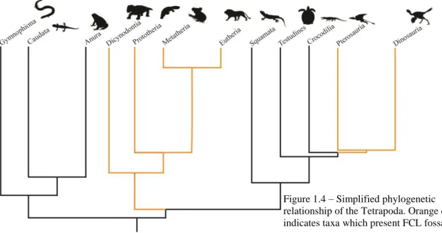
Figure 1.4 – Phylogenetic context of the FCL fossa………6

Figure 2.1 – Micro-CT setup………11

Figure 2.2 – Specimen preparation………...………..11

Figure 2.3 – Segmentation of the FCL…………..………..18

Figure 2.4 – Segmentation of the semicircular canals………...…...20

Figure 2.5 – Measurement of the semicircular canals….………...…..20

Figure 2.6 – FCL and brain size correlation (mammals)………...……..23

Figure 2.7 – FCL and brain size correlation (birds)………...…..24

Figure 2.8 – OL and brain size correlation………..………...……..25

Figure 2.9 – Mammal phylogeny………..….26

Figure 2.10 – Bird phylogeny……….………..………..27

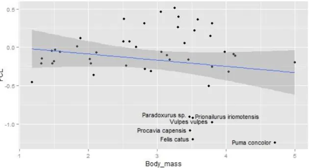
Figure 3.1 – FCL vs bodymass scatterplot (mammals)………..………..………...31

Figure 3.2 – FCL vs feeding ecology scatterplot (mammals)……….………31

Figure 3.3 – FCL vs locomotor type scatterplot…………..………...…………..32

XIV

Figure 3.5 – FCL vs agility scatterplot………..………..33

Figure 3.6 – FCL vs circadian activity pattern scatterplot (mammals)……….…...………..33

Figure 3.7 – FCL vs anterior semicircular canal scatterplot………...…………34

Figure 3.8 – FCL vs circadian activity pattern scatterplot (birds)………..34

Figure 3.9 – FCL vs feeding ecology scatterplot (birds)..………..35

Figure 3.10 – FCL vs bodymass scatterplot (birds)..……….…..………..35

XV Table Index

Table 1.1 – General divisions of the cerebellum………..………....……2

Table 2.1 – List of mammalian specimens………...…..12

Table 2.2 – List of bird specimens……….…………..14

Table 3.1 – Results (mammals)………...……….29

Table 3.2 – Results (mammals II)………...….30

Table 3.3 – Results (birds)………...…….30

XVII

Abbreviations and acronyms list

ASC – Anterior Semicircular Canal

BrainR – Brain reduced (Total Endocast Volume minus FCL) Brainr – Brain reduced (Total Endocast Volume minus optic lobes) CT – Computed Tomography

FCL – Floccular Complex Lobe

HZB – Helmholtz Zentrum Berlin, Berlin, Germany

KUPRI – Kyoto University Primate Research Institute, Kyoto, Japan MfN – Museum für Naturkunde, Berlin, Germany

ML – Museu da Lourinhã, Lourinhã, Portugal OL – Optic Lobes

PGLS – Phylogenetic Generalized Least-Squares Q-Q – Quantile-Quantile

VCR – Vestibulo-collic reflex VOR – Vestibulo-occular reflex

1

Figure 1.1 – Scheme of the development of the cerebellum, showing the early differentiation of the vestibulocerebellum of Homo sapiens. Brain at the end of the 5th week (A); sagittal section of the hindbrain at the age of 6 weeks (B); sagittal section of the hindbrain at the end of the 17th week. Phylopic.org silhouette – credits to T. Michaels Keesey.

Introduction

The full range of sensations that allow us to feel the world, along with its consequent set of actions (behavior), is processed and determined by a combination of neuronal circuits that exist in our nervous system. A central paradigm in neuroanatomy assumes that the volume of a certain neuroanatomical structure is proportional to its functional importance. This is the principle of proper mass (Jerison, 1973). This principle refers that the evolution of intelligence is a result of increasing information processing capacity and that the latter is correlated with the amount of brain tissue (Jerison, 1973). The study here proposed exploits this general rule and highlights the complexity and integration of neuronal tissues.

A review of the anatomy, histology, development and evolutionary framework of the cerebellum

Within the central nervous system, the cerebellum is particularly interesting. It regulates movement coordination, cognition and perception (Paulin, 1993). The cerebellar cortex is composed by four main types of neurons: Purkinje cells, granule cells, Golgi cells and stellate cells (Voogd & Glickstain, 1998). The cerebellum has two major inputs (mossy fibers and climbing fibers) and one single output (composed by Purkinje cells), and appears, therefore, to be a simple circuitry (Voogd &

2 Wylie, 2004). Granule cells, the most numerous cells in the cerebellar cortex, are contacted by mossy fibers via complex synapses on their dendritic terminations and their axons extend to the superficial layer of the cerebellar cortex, terminating either on dendrites of interneurons or Purkinje cells (Voogd & Glickstein, 1998). The cerebellum in hagfishes and lampreys is simply a group of modified cells of the acusticolateral area of the medulla oblongata (Johnston, 1901 in Larsell, 1967). In urodeles, the cerebellar structure is similar to those of hagfishes and lampreys but the corpus cerebelli, which receives proprioceptive and other sensory impulses, becomes more developed and eventually the predominant feature of the cerebella of selachians, teleosts and all amniotes (Larsell, 1967).

Table 1.1 – General divisions of the cerebella of mammals and birds according to Ziehen (1899)

Vermis lobules Hemispheral lobules Folia

Lingula Vinculum lingulae I

Lobulus centralis Ala lobuli centralis II & III

Culmen Lobulus quadrangularis (Pars anterior)

IV & V Declive Lobulus quadrangularis (Pars

posterior)

VI

Folium vermis Lobulus semilunaris superior VII A

Tuber vermis Lobulus semilunaris inferior VII B

Pyramis Lobulus biventer VIII

Uvula Tonsilla (dorsal paraflocculus) IX

3

Figure 1.2 – Schematic illustration of a Microcebus murinus floccular complex with bones of the periotic complex transversally cut (dorsal view) (above); schematic illustration (parasagittal section) of an adult

Columba livia cerebellum (adapted from Larsell, 1967) with identification of the 10 folia listed on table

4 During development, the ectodermal plate (Figure 1.1) begins folding dorsally, which originates the formation of the neural tube. The closure of the rostral neuropore originates the three primary brain vesicles: the prosencephalon (forebrain), the mesencephalon (midbrain) and the rhombencephalon (hindbrain) (Gilbert, 2010; Shekdar, 2011). Neural tube bending develops two flexures - cephalic and cervical – and later a new dorsal flexure is developed in the middle of the former two – the pontine flexure – thus dividing the rhombencephalon in two portions, the metencephalon and the myelencephalon (Gilbert, 2010; Shekdar, 2011). The cerebellum originates from both the rostral portion of the metencephalon and the caudal portion of the mesencephalon (Hallonet et al., 1990; Christensson, 2007; Fotos et al., 2011). It can be divided into three parts: the vestibulocerebellum (or archicerebellum), which is the phylogenetically oldest part of the cerebellum and has connections with the vestibular apparatus; the paleocerebellum, which is phylogenetically more recent than the vestibulocerebellum and is related to density data from limbs; the neocerebellum, which controls limb movements and is the part of the cerebellum that appeared more recently in the evolution of the brain (Voogd & Glickstain, 1998; Shekdar, 2011). The cerebellum is a folded structure typically divided in folia (Larsell, 1967; Voodg & Glickstein, 1998). The nomenclature here used is presented in table 1.1 (see Figure 1.2). This work will focus on the vestibulocerebellum, which

Figure 1.3 – Schematic illustration of a coronal section of a cerebellum of a Scyliorhinus canicula (Adapted from Pose Mendez (2013)). It is possible to see the auricle, which corresponds to the FCL, and the immediately adjacent octavorateral area, which functions are related with to detection of vibrational signals by the octavolateral system (which comprises the ear and the mechanosensory lateral line). Phylopic.org silhouette uncredited.

5 includes the flocculus, paraflocculus, nodulus and uvula, or simply: the floccular complex (Figures 1.2) that correspond to folia IX and X of Ziehen (1899) nomenclature (Larsell, 1967; Voogd & Glickstain, 1998; Kheradmand & Zee, 2011). It is difficult to establish homologies between specific folia in phylogenetically distant taxa but the basic functions of the floccular complex are common to all cerebella. This happens because the basic cerebellar divisions in all gnathostomes consists of auricles (which corresponds to the FCLs) and cerebellar body (Larsell, 1967; Paulin, 1993; Pose Mendez, 2013). According to Pose Mendez (2013), the upper and lower auricle leaves of the cerebellum of cartilaginous fishes are homologous to the vestibulocerebellum. Studies suggest that the upper auricle leaf (Figure 1.3) is homologous to the X folium of the amniote cerebellum, which corresponds to the flocculus and nodulus (Pose Mendez, 2013). In general, the eminentia granularis (a part of the vestibulolateral lobe of fish and amphibians cerebella that is the location of some nerve synapsis of the lateral line) performs functions related to vestibular and proprioceptive perceptions in fishes and even in anurans. Nevertheless, it is the torus longitudinalis (granular cells that develop in the cerebellum of teleost fishes) that is presumed to control posture, detect luminance levels and monitor saccadic movements in teleosts (Kotrschal et al., 1998; Albert, 2001). Larsell (1967) refers that the modified eminentia granularis of anurans is homologous to flocculi of birds and mammals.

The floccular complex of the cerebellum

The floccular complex of the cerebellum is a center for integration of visual and vestibular stimuli while controlling the extraocular muscles (Zee et al., 1981; Voogd & Wilie, 2004). There is a connection between the axes of the three semicircular canals, the three extraocular muscles and the rotation axes of the field of view, because floccular zones project to extraocular motorneurons, via cerebellar nuclei, which causes eye rotation according to the best response axis of the climbing fibers (De Zeeuw et al., 1994 in Wylie et al, 1994). The compartmentalization of the flocculus reflects the monitoring of eye rotation, because each compartment projects to two of the extraocular muscles (Winship & Wylie, 2003).

Several studies have focused on the retina image stabilization function (Ito, 1982; Nagao, 1992; Nagao et al, 1997; Winship & Wylie, 2003). The vestibulocerebellum‟s floccular complex is involved in posture, balance and head/eye movements control (Paulin, 1993; Netter et al., 2002). In mammals and birds, the vestibulocerebellum is composed by the: flocculus, paraflocculus, nodulus and ventral uvula (Larsell, 1967; Ito, 1982; Angelaki & Hess, 1994). The floccular complex regulates compensatory movement of the eyes to respond to rotational movements of the head (vestibulo-ocular reflex, VOR), or to track a moving object in the field of view (smooth pursuit) and also contributes to stabilize the head via cervical muscles (vestibule-collic reflex, VCR) (Ito, 1982; Waspe et al., 1983; Burdess, 1996; Voogd & Wylie, 2004). The flocculus/paraflocculus responds to brief vestibular stimuli, sustaining pursuit eye movements and gaze holding, while the nodulus/ventral uvula act during sustained vestibular responses (Kheradmand & Zee, 2011). VOR processing can adapt and

6 learning allows the reduction of error in rapid responses during flight speed alterations, acrobatic maneuvers in aquatic environments or prey tracking during high-speed pursuit predation (Ito, 1998; Witmer et al., 2003, Walsh et al., 2013). A signal is transferred from mossy fibers afferents to Purkinje cells and this signal can be “corrected” because of a unique dual input system existing in the cerebellum (Ito, 1982). Given the retinal errors, neuronal networks of the floccular complex may be reorganized by the visual climbing fiber afferents, resulting in improvement and adaptation of the VOR (Ito, 1982).

The present work focuses on the lateral projections of the cerebellum that comprise the flocculus and paraflocculus. Several terminologies have been used to refer both to the FCL and the fossa housing it, flocculus, paraflocculus, cerebellar auricula, fovea floccularis (Olson, 1944; Larsell, 1967; Hopson, 1979; Gannon et al., 1988; Ivakhnenko, 2008; Castanhinha et al., 2013). For simplicity and correction, and because I used bird and mammal endocasts, I will hereinafter refer to these lateral projections as floccular complex lobes (FCLs).

The FCLs protrude into the periotic and prootic bones (in mammals and birds, respectively) and are housed in the FCL fossa (Figure 1.2). FCL fossae are present in distinct groups of animals such as: dinosaurs (birds, non-avian theropods, ornithopods, sauropods) (Franzosa, 2004; Miyashita et al, 2011; Walsh et al., 2013; Thomas, 2015) pterosaurs (Witmer et al., 2003) mammal-like reptiles (Olson, 1944; Castanhinha et al., 2013; Laaß , 2015) and mammals (Olson, 1944; Gannon, 1988) (Figure 1.4). I assume that the FCL fossa volume is a good proxy to access the FCL volume as it is assumed that bird and mammal endocasts are good aproximations of brain morphology and size (Jerison, 1973; Hopson, 1979; Gannon, 1988; Iwaniuk & Nelson, 2002; Macrini et al., 2007). In fact, Edinger (1948 in Lyras, 2009) comments that the study of brain external morphology with endocasts provides, in most mammals, more reliable information than real brains.

Figure 1.4 – Simplified phylogenetic relationship of the Tetrapoda. Orange color indicates taxa which present FCL fossae.

7 Paleobiological speculations on the floccular complex function

There are several examples in the literature of direct or indirect association between FCL fossae size and high maneuverability and agility in birds (Milner & Walsh, 2009; Walsh & Milner, 2011), dinosaurs (Domínguez et al., 2004, Franzosa, 2004), and pterosaurs (Witmer et al., 2003). Therapsid large FCL fossae casts have also been associated to an active life style (Olson, 1944; Laaß, 2015), as well as to locomotion in three-dimensional environments such as aquatic environments (Ivakhnennko, 2008). In addition, Gannon (1988) noted a correlation between the increase of FCL fossae relative size and the decrease of body mass in mammals.

There are, however, some issues about the FCL function that may blur the analysis of the FCL size variation, namely the plasticity of the cerebellum and its unclear functional compartmentalization. Although FCLs are functionally related to eye movement and image stabilization, eye motor control is not exclusively performed by these lobes, but also by the ventral uvula, nodulus or oculomotor vermis, for example (Rambold et al., 2002; Kheradman & Zee, 2011).

Nevertheless, some interesting speculations have been proposed about the FCL and ecology. Franzosa (2004) observed that theropod dinosaur brain specimens tended to decrease in size and therefore body mass and suggested that during theropod evolution there was an enlargement of the optic lobes and cerebral hemispheres. Franzosa (2004) also suggested that as optic lobes increase, FCLs also increased in size. This would be explained by the fact that theropods became active predators (instead of scavengers) and a decrease in prey size demanded more speed and agility from the predator (Hopson, 1980). Increased optic lobes, cerebral hemispheres and FCLs size indicates that there was a selective pressure for improved agility and hand-eye coordination in theropods (Russel, 1969; Pearson, 1972). The conspicuity of the FCLs has also been related to the acquisition of flight capacity (Domínguez et al., 2004) which, once again, relates agility/maneuverability and the relative size of these structures.

Other than eye motor control functions were suggested by Witmer et al. (2003) for pterosaurs. It was hypothesized that the large FCLs of Rhamphorhynchus muesteri and Anhanguera santanae were related to processing of proprioceptive and somatosensory information produced by the membranous wings (Witmer et al., 2003). This suggestion was based on Winship & Wylie (2003) study. However, evidence to support such speculation is not clear. In primates, Gannon (1988) noted a negative correlation between body mass and FCL relative size. Great apes (e.g., Homo sapiens) lose the FCL fossa after birth, only remaining a smaller accessory paraflocculus (Spoor & Leakey, 1996). Probably, large FCLs are plesiomorphic to extant mammals (Kielen-Jaworowska, 1986). Olson (1944) briefly discusses variation in FCL fossa depth and refers that smaller and very active animals have large FCLs and tend to have large periotic bones. This could represent that the FCLs size is conditioned by a more complex set of morphological constraints. Paulin (1993) argues that FCLs function in bats may be associated with echolocation instead of eye movement control. The idea that

8 FCLs have other functions besides eye motor control (Paulin, 1993; Witmer et al., 2003) are supported by the cerebellum evolutionary history (Larsell, 1967) and its plasticity, and will be discussed later on.

Testing paleobiological speculations

I will use CT-scanned braincase endocasts (Balanoff et al., 2015) of extinct and extant species to test the relation between the relative volumes of the FCL fossa under the following hypotheses:

Hypothesis I, larger animals present proportionally smaller FCL. Rationale: the amount of neural tissue required to process a certain neural input might have a limit so in animals with bigger brains the quantity of neurons present in the a large cerebellum might be enough to process all the required inputs without the need of producing a larger FCL fossa (Gannon, 1988; Franzosa, 2004);

Hypothesis II, slower animals have smaller FCL fossae; Rationale: animals with more agility should need a larger amount of neural tissue to process visual and vestibular stimuli to improve image stabilization accuracy (Olson, 1944; Franzosa, 2004);

Hypothesis III, different locomotion strategies correspond to different FCL size patterns; Rationale: similar to Hypothesis II with a different categorization;

Hypothesis IV, feeding habits can be correlated with FCL size. Rationale: niches which primarily require an optimized vision should be occupied by animals with efficient eye movements (Hopson, 1980);

Hypothesis V, size of FCL and optic lobes of birds are positively correlated. Rationale: increased FCL fossa volumes suggest a better vision acuity and are possibly associated with enlargement of the optic lobes in vision-dependent animals (Franzosa, 2004);

Hypothesis VI, animals with different circadian activity patterns present different FCL sizes. Rationale: given the different level of reliance in vision of diurnal and nocturnal animals, there is a difference between FCL relative sizes in these two groups.

Hypothesis VII, size of FCL and area and perimeter of the anterior semicircular canal (ASC) are positively correlated. Rationale: since the FCLs are constricted by the ASC, it is expected that larger relative ASC areas and perimeters correspond to larger relative FCLs.

I will here discuss, basing on the results for each hypothesis, the reported assumptions that FCL fossa volume can shed light on animal ecology.

9 Material and Methods

Important concepts of statistical analyses

This section aims to facilitate the interpretation of the Materials and Methods section. The topics/concepts are ordered according to the order of appearance on the text.

Logarithmic base-10 transformation – Parametric statistical tests require data or residuals to be normally distributed, thus the original data may need to be transformed to meet such assumptions. Therefore, it is possible to perform a mathematical operation to transform data, thus it may fit a parametric statistical test, such as an Anova or a linear regression (McDonald, 2014). Many biological variables have log-normal distribution, which means that data is normal after a logarithmic transformation (McDonald, 2014). Logarithmic transformations are commonly used to transform size data and, by using a Log 10 transformation it is easy to see the magnitude of the original number (e.g., log(10)=1, log(100)=2, etc.) (Spoor et al., 2007; Walsh et al., 2013; McDonald, 2014). I here used base-10 log transformation to normalize data.

Linear regression / Residuals – When a linear regression is computed, each of the observed values of the predictor (x) and response (y) variables create a line showing a trend of the values along the x and y axes. This line is given by y=mx+b, where m is the estimated slope and b is the estimated intercept (value of y when x=0) (Verzani, 2014). To each data point there is a corresponding estimation, which is a point of the estimated regression line (Verzani, 2014). The difference between the response variable observed value and the predicted value (given by the interception of the regression line and the corresponding predictor value) is called a residual (Verzani, 2014). Geometrically, a residual is the vertical distance of a given point (xi,yi) to the regression line.

Generalized Least-squares – GLS is a technique to estimate unknown parameters of a linear regression model. When a regression line is produced in a graph, it minimizes the squared vertical distances between the data points and the line (Greene, 2003; McDonald, 2014). To each xi of a data

point corresponds a yi and an estimation, ̂. The difference between yi and ̂ is calculated and squared

and the sum of the squared deviates of all data points is a measure of how well the regression line fits the data (Greene, 2003; McDonald, 2014). Among the pool of possible lines to fit the data, the regression line is the chosen one with the smallest sum of squared deviates. It may happen that errors (or disturbances) have a non-constant variance (heterokedastic) or are correlated (autocorrelation) and in that case a Generelized Least-squares estimator can be used, converting a heterokedastic into a homokedastic model (Greene, 2003). For further reading on the theory of Generalized Least-squares estimation see chapter 10 of Econometric Analysis that deals with the detailed mathematics details involved in this process (Greene, 2003).

Prediction interval – In regression analysis there are two types of interval usually referred: confidence intervals and prediction intervals. Confidence intervals are related with estimation of parameters and contain all the null hypotheses that would not be rejected given a α% significance level

10 (Faraway, 2002). In practice, confidence intervals are related with the regression line and contain the parameter values that should not be rejected.

A prediction interval gives an estimate of a range of values where future observations will fall, taking into account the analyzed sample, with a confidence of 100(1-α)% (Garland and Ives, 2000). In this case, instead of a parametric distribution, the intervals predict the distribution of individual future points. On both cases there are two limits, the upper and the lower, which are frequently represented in regression plots (e.g., Figure 2.6).

Collinearity – Collinearity or multicollinearity among predictors (independent variables) is not desirable (Mundry, 2014). When two predictors, or a group of more than two, are strongly correlated, they provide the same information, which means they are redundant variables (Mundry, 2014). Collinearity has two main consequences: 1) conclusions about collinear predictors are unreliable, with increased standard errors of parameter estimates and unreliable non-significance (P > 0.05) being the main problems; 2) a model with collinearity is unstable and results can be altered by small changes (Mundry, 2014). To address this, the inspection of variance inflation factors and consequent drop of the problematic variable(s) is advisable (Mundry, 2014).

Covariance matrix – A covariance matrix (or variance-covariance matrix) is a theoretical matrix derived from a phylogenetic tree which quantifies species divergence from their common ancestor (variance) and resemblance among species (covariance) (Paradis, 2011). A matrix of this type is therefore essential to perform Phylogenetic Generalized Least-squares analysis, thus improving the linear model.

Ultrametric tree – Phylogenetic trees have branches which represent some kind of distance between species. These branch lengths have variable distance types, depending on data type and resources available to build a tree. An ultrametric phylogenetic tree is the one in which all tips (species) are equally distant from the common ancestor.

11 Micro-CT scans

A total of 47 extant mammal species and 1 Anomodontia species were selected to cover the widest ecological range possible (see Table 2.1). From these, I scanned 27 skulls from the mammal collections of the Museum für Naturkunde (MfN) at the micro-CT in Helmholtz Zentrum Berlin (HZB) (see Figure 2.1). The

selected skulls were placed into cylindrical plastic

containers and

accommodated with pieces of styrofoam, both to protect the specimen‟s fragile structures and avoid displacement from the original position (see Figure 2.2). X-ray µCT scanning was performed with a micro-focus 150 keV

Hamamatsu X-ray source with a tungsten target and a flat panel detector C7942 (120x120 mm, 2240×2368 pixel, pixel size 50 µm). All the specimens were scanned with an acceleration voltage of 100 keV and a beam current of 95 µA with an exposure time of 0,5 seconds. Image noise was reduced by using a 3-fold integration. The source-object distance was 220 mm and a source-detector distance of 300 mm was used, thus achieving a magnification factor of 1.36. The number of acquired projections varied between 800 and 1000. In the X-ray cabinet the sample was rotated in a precision rotation stage from Huber, Germany. I used Octupus V8.6 software to implement the back-projection algorithm with convolution and correction for cone beam. The average voxel size of the reconstructed volumes was 36,8 µm. The resulting data sets were binned (2x2x2, average binned) using software FIJI (Schindelin et al., 2012). This process performs an eight-fold reduction of data size to facilitate processing and handling.

Figure 2.1 – Micro-CT setup at the HZB.

Figure 2.2 – Cylindrical plastic containers pilled and glued, with specimens inside.

12

Table 2.1 – List of mammal and anomodont species used in this study and their meausured FCL fossae volume, braincase endocast volume, and FCL % of the endocast. Volumes result from the sum of both left and right FCLs. Species are ordered and phylogenetically grouped.

Species Common name FCL volume (mm3)

Endocast volume (mm3)

FCL %

Ornithorhynchus anatinus Platypus 56,63 9732,84 0,58

Cebus apella Tufted capuchin 252,58 68123,24 0,37

Brachyteles arachnoides Southern muriqui 232,07 110426,26 0,21

Lagothrix lagotricha Humboldt‟s

woolly monkey

561,00 95153,29 0,59

Alouatta caraya Black Howler 257,75 48899,50 0,53

Hylobates agilis Agile gibbon 90,56 105684,25 0,09

Otolemur crassicaudatus Brown greater

galago

50,05 9926,55 0,50

Presbytis melalophus Sumatran surili 130,58 73154,19 0,18

Microcebus murinus Grey mouse

lemur

25,13 1549,58 1,62

Varecia variegata Black-and-white

ruffed lemur

328,99 32013,42 1,03

Propithecus verreauxi Verreaux's sifaka 199,94 23437,61 0,85

Lepus capensis Cape hare 263,81 12106,82 2,18

Idiurus macrotis Long-eared

Flying Mouse

10,42 836,64 1,25

Anomalurus derbianus Lord Derby's

scaly-tailed squirrel

116,95 6655,76 1,76

Ondatra zibethicus Muskrat 39,59 4524,33 0,88

Arvicola terrestris European water

vole

8,73 1124,55 0,78

Mus musculus House mouse 3,81 390,18 0,98

Rattus norvegicus Brown rat 15,86 1904,64 0,83

Dipodomys deserti Desert kangaroo

rat

18,50 1766,76 1,05

Marmota marmota Alpine marmot 145,96 11615,83 1,26

Sciurus vulgaris Red squirrel 126,64 6151,98 2,06

Ratufa bicolor Black giant

squirrel

203,25 12005,61 1,69

Ratufa affinis Cream-coloured

giant squirrel

206,51 9686,79 2,13

13

Vulpes vulpes Red fox 19,65 50355,69 0,04

Ursus americanus American black

bear

296,54 238402,84 0,12

Lutra lutra European otter 84,43 44655,21 0,19

Meles meles European badger 133,27 40130,94 0,33

Paradoxurus sp. Palm civet 13,71 20450,59 0,07

Prionailurus iriomotensis Iriomote cat 18,24 34932,50 0,05

Felis catus Domestic cat 8,31 27506,92 0,03

Puma concolor Cougar 23,07 187732,02 0,01

Rousettus aegyptiacus Egyptian fruit bat 25,64 2221,33 1,15

Pteropus giganteus Indian flying fox 33,48 8963,99 0,37

Rhinolophus ferrumequinum Greater horseshoe bat

6,21 351,52 1,77

Diphylla ecaudata Hairy-legged

vampire bat

13,63 690,72 1,97

Desmodus rotundus Common vampire

bat

16,40 910,69 1,80

Molossus rufus Black mastiff bat 7,61 437,80 1,74

Procavia capensis Rock hyrax 7,23 13980,43 0,05

Potamogale velox Giant otter shrew 22,20 3968,67 0,56

Oryzorictes sp. Rice tenrec 11,10 521,63 2,13

Dasyurus hallucatus Northern quoll 45,51 3339,75 1,36

Petaurus sp. Flying phalanger 46,38 3444,60 1,35

Phascolarctos cinereus Koala 110,78 26275,29 0,42

Dromiciops gliroides Monito del monte 11,87 821,00 1,45

Monodelphis domestica Gray short-tailed

opossum

11,34 956,06 1,19

Didelphis virginiana North American

opossum

39,17 6608,01 0,59

Niassodon mfumukasi (ML ML1620

14

Table 2.2 – List of bird species used in this study and their meausured FCL volume, braincase endocast volume, and FCL % of the endocast. Volumes result from the sum of both left and right FCLs and OLs. Endocast and FCL volumes from Walsh et al. (2013). Species are ordered and phylogenetically grouped.

Species Common name FCL volume (mm3) Endocast volume (mm3) Optic lobes volume (mm3) FCL % Rhynchotus ruficens Red winged tinamou 14,86 3690,58 439,92 0,40

Apteryx haastii Great spotted kiwi 32,24 12496,13 88,72 0,26 Dromaius novaehollandiae Emu 236,13 27054,5 2002,03 0,87 Casuarius casuarius Cassowary 271,95 32724,27 2274,34 0,83

Struthio camelus Ostrich 195,92 36517,99 2585,47 0,54 Rhea americana Greater rea 153,76 13713,05 1364,45 1,12 Phasianus

colchicus Common

pheasant

29,78 4021,23 530,80 0,74

Gallus gallus Red junglefowl

35,87 3976,07 452,87 0,90

Cygnus olor Mute swan 149,53 17360,36 447,90 0,86 Aythya fuligula Tufted duck 38,97 5351 277,72 0,73 Tachyeres brachypterus Falkland steamer duck 92,15 6667,4 288,03 1,38 Phaethon lepturus White tailed tropic bird 40,5 2803,58 408,48 1,44 Opisthocomus hoazin Hoatzin 33,33 3370 194,79 0,99 Podiceps cristatus Great crested grebe 44,61 3303,11 334,27 1,35

Gavia immer Great northern loon 179,58 12284,93 829,23 1,46 Pelagodroma marina White faced storm petrel 3,92 496,91 51,28 0,79

15 Diomedea exulans Wandering albatross 192,4 29151,6 760,86 0,66 Pelecanoides urinatrix Common diving petrel 64,3 1351,72 90,29 4,76 Fulmarus glacialis Northern fulmar 48,96 7440,16 174,10 0,66

Eudyptula sp. Little penguin 64,3 8522,17 557,35 0,75 Ciconia ciconia White stork 56,15 11348,13 820,47 0,49 Threskiornis

aethiopicus

Sacred ibis 54,17 9643,49 428,17 0,56

Ardea cinerea Grey heron 69,61 4999,82 388,49 1,39 Pelecanus erythrorhynchos American white pelican 105,12 13012,42 356,54 0,81 Fregata magnificens Magnificent frigate bird 66,31 10402,14 422,33 0,64 Phalacrocorax carbo Great cormorant 82,2 13440,04 532,23 0,61 Phalacrocorax harrisi Galapagos cormorant 71,37 10936,73 708,70 0,65

Grus grus Common crane

166,06 19959,78 1157,67 0,83

Columba livia Rock dove 14,84 2134,52 222,20 0,70 Creagrus

furcatus Swallow

tailed gull

25,22 4927,97 327,71 0,51

Larus argentatus Herring gull 30,4 5719,9 602,88 0,53 Rhynchops niger Black

skimmer 8,45 1235,81 83,79 0,68 Gelochelidon nilotica Gull billed tern 17,36 1900,16 182,04 0,91

Stercorarius skua Skua 53,89 6785,19 402,36 0,79 Alca torda Razorbill 47,04 3285,72 197,80 1,43 Vultur gryphus Condor 383,23 27099,93 899,72 1,41

16 Circus cyaneus Hen harrier 25,86 3928,72 478,91 0,66 Buteo buteo Common

buzzard

33,22 7856,74 766,82 0,42

Aquila chrysaetos Golden eagle 104,74 21045,03 1073,30 0,50 Pandion haliaetus Osprey 80,57 10151,38 556,30 0,79 Sagittarius serpentarius Secretary bird 124,33 12912,27 1035,56 0,96

Tyto alba Barn owl 22,65 6522,84 113,50 0,35 Trogon curucui Blue crowned

trogon 6,33 890,72 88,09 0,71 Coracias garrulus European roller 12,70 1970,03 280,34 0,64

Alcedo atthis Common kingfisher 8,12 741,51 98,99 1,10 Ramphastos dicolorus Toucan 34,45 4525,02 466,53 0,76 Falco tinnunculus Common kestrel 20,17 3154,65 286,44 0,64

Falco subbuteo Eurasian hobby

18,65 2994,73 256,95 0,62

Amazona aestiva Blue fronted amazon

35,24 8511,51 305,56 0,41

Ara macao Scarlet

macaw 29,08 15157,87 715,45 0,19 Strigops habroptila Kakapo 26,06 8849,56 30,09 0,29 Tyrannus tyrannus Eastern kingbird 1,18 532,71 59,58 0,22 Acanthorhynchus superciliosus Western spinebill 28,89 2369,64 318,24 1,22

Corvus corax Raven 1022,46

17 Podargus strigoides Tawny frogmouth 14,84 2322,97 239,67 0,64 Selasphorus rufus Rufus hummingbird 1,64 157,29 17,60 1,04

Apus apus Common

swift

5,25 707,83 50,89 0,74

Steatornis caripensis

Oilbird 14,55 2039,77 103,32 0,71

Brain and FCL endocast segmentation protocol

The data were processed using Amira 5.3.3 (Visualization Sciences Group. France). Processing consisted of five parts: 1) reorientation of the scan to obtain digital skulls in orthogonal anatomical orientation by using the Transform Editor and applying the transformation using a standard interpolation in extended mode and preserving voxel size; 2) bone segmentation by using the Masking tool of the Segmentation Editor to select all bone material in each slice; 3) manual segmentation of the braincase cavity using “Magic Wand” or “Brush” tools; 4) selection of both FCL fossae volumes by using the 3d “lasso” tool – this process consisted of 3 steps: a) making a sagittal cut of the skull which made the periotic area visible; b) selecting the volume inside the fossae; c) cut the volume that exceeds the contour (corresponding to the anterior semicircular canal) that results from the change of angle between the braincase lateral wall and the fossa itself (Walsh et al., 2013) (Figure 2.3); 5) measurement of brain cavity and FCL fossae volumes (combined volume of left and right structures). The FCL fossae volumes were measured trice by different people in order to detect relevant measurement errors. No significant differences were noticed between different measurements. This procedure was applied to all CT scans.

Braincase cavity and FCL fossae volumes for Monodelphis domestica. Didelphis virginiana. Phascolarctos cinereus. Dasyurus hallucatus and Dromiciops gliroides were obtained from Macrini at el. (2007). I used Castanhinha et al. (2013) values and semicircular canal images of Niassodon mfumukasi.

17 skull CT scans were downloaded from the Kyoto University Primate Research Institute‟s (KUPRI) online collection (http://dmm.pri.kyoto-u.ac.jp/). Although the voxel size of these scans was larger it did not compromise our analysis, because the resolution allowed detection and a detailed segmentation of the FCLs fossae. These specimens were not used to perform measurements with the semicircular canals because scan quality did not allow for an accurate selection of these structures.

Our bird dataset is composed of 59 species of extant birds (Table 2.2). I used published FCL fossae cast and endocast volumes (Walsh et al. 2013). The optic lobes (OL) are part of the

18 mesencephalon (midbrain) and are especially prominent in birds (Alonso et al., 2004; Kundrát. 2007). which makes them distinguishable and possible to separate from the rest of the brain structures. I used a similar protocol to the one described above for mammals to digitally segment the FCL volumes.

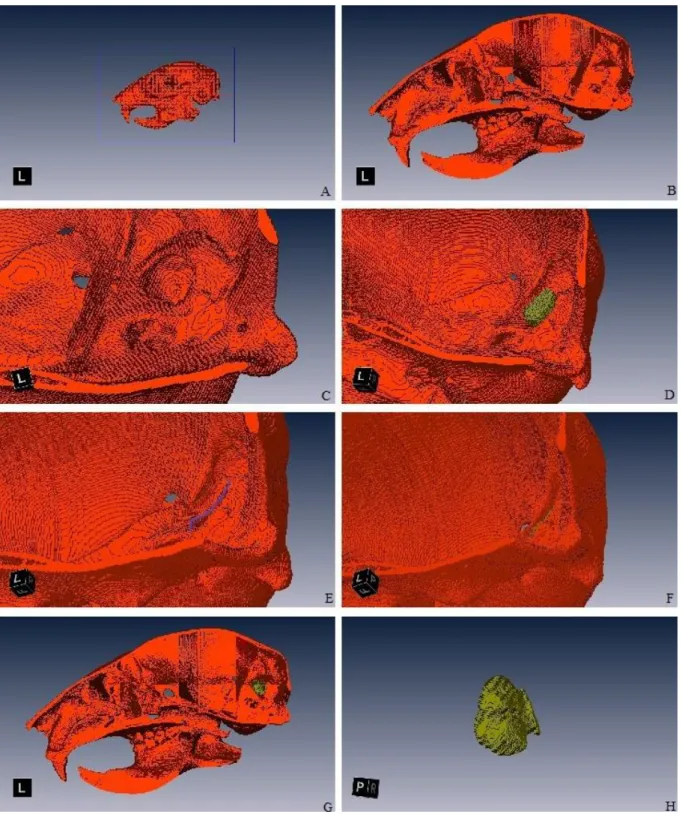
Figure 2.3 – Segmentation process of FCLs: lateral view of a Sciurus vulgaris (red squirrel) skull (A); sagittal view after cutting the proximal part of the skull (B); detail of the periotic and the FCL fossa (C); volume of the FCL fossa roughly selected (D); selection of the plane delimiting the fossa (E); extraction of the exceeding volume (F); sagittal view of the skull with FCL fossa volume selected (G); a cast of the FCL fossa (H).

19 Semicircular canals segmentation protocol

The segmentation of the semicircular canals was only performed on the MfN specimens because the quality of the CT-scans allowed a satisfactory reconstruction of these structures. To improve resolution in some of the smaller animals the original (non-binned) data was used for semicircular canals segmentation. The process was similar to braincase cavity segmentation and consisted of the first three parts of the abovementioned procedure. In most cases, the threshold of the masking tool was adjusted multiple times during semicircular canals manual segmentation. This was important because some parts of these small structures could not be selected with the same threshold values used to segment the braincase cavity. After segmentation, a 3D image of each anterior semicircular canal was created using “SurfaceGen” function with constrained smoothing of the surface and a minimal edge length of 0,4. The surface was displayed with the “SurfaceView” module and the following setting was applied: “Draw style” was defined as Shaded, which displays an opaque shaded surface with no visible edges; in “More options”, I selected Opaque, Both faces; the last group options I selected Direct normals and used constrained smoothing in the surface rendering.

Then the perspective was changed to orthographic and the “two viewers” option was enabled to allow the visualization of the surface from two different angles. I oriented the anterior semicircular canal on a longitudinal plane on the first camera using the transform editor trackball manipulator to obtain a sagittal view on the second camera because the camera positions are positioned at 90º, (see Figure 2.4). A scale was then created and the background was turned black in order to increase contrast. Then I produced snapshots and opened the resulting images using FIJI (Schindelin et al.. 2012). Using “Set scale” function to define a reference known distance I calibrate them. Then I selected the “Wand” tool and set tolerance to 10 to select the inner area outlined by the anterior semicircular canal (see Figure 2.5). In order to obtain a smoother selection, all the forms were interpolated before being measured using an interval of 20 pixels. I used “Measure” from “Analyze” menu to obtain area and perimeter values.

20

Figure 2.5 – Measurement of a Lutra lutra (European otter) anterior semicircular canal area and perimeter.

Figure 2.4 – Reorientation process of the anterior semicircular canal of Ratufa bicolor (Black giant squirrel) with double view option and “trackball” transformation tool.

21 Statistical analysis

To obtain relative values for FCL, optic lobes and anterior semicircular canal areas I performed a log 10 transformation on the original FCL, optic lobes (OL), Total Endocast Volume minus FCL (BrainR) and Total Endocast Volume minus optic lobes (Brainr), anterior semicircular canal areas (ASC) and calculated phylogenetic residuals from linear phylogenetic regressions on: FCL and BrainR for mammals and birds; OL and Brainr for birds; ASC and BrainR. To calculate these residuals I used R package phytools (v 0.3-72) that fits phylogenetic regressions and computes the residuals which was designed for phylogenetic size correction using GLS regression (Revell, 2009). This package requires the input of a dependent (e.g., FCL volume) and at least an independent variable (e.g., BrainR volume) as well as a phylogenetic tree (see below) in R‟s “phylo” format which can be loaded both on Nexus or Newick file formats. The phylogenetic residuals obtained were used as relative FCL, OL and ASC size in the subsequent analyses. Residuals were analyzed and normality was tested, following Butler et al. (2000), using histograms, Q-Q plots and Shapiro-Wilk normality tests. In all situations I used PDAP package (Garland et al.. 1993) in Mesquite 3.03 (Maddison & Maddison. 2009) to run phylogenetically correct regressions and map the prediction intervals onto the original tip data space (see Figures 2.6, 2.7, 2.8) to detect the existence of outliers before the analyses (Garland & Ives. 2000). For OL relative values calculation Apteryx haasti (great spotted kiwi) and Strigops habroptila (kakapo) were dropped because they were significant outliers, i.e., they fell out of the phylogenetic prediction interval. Body mass values for birds were obtained from Walsh et al. (2013) and from Felisa et al. (2003) for mammals. These values were also log 10 transformed.

I built a phylogenetic tree (Figure 2.9) based on the topology of Meredith et al. (2011). Mesquite 3.03 was used to build the tree and modify branch lengths. I used divergence time as branch lengths and data was collected from several publications. Spoor et al. (2007) was used for higher taxonomic levels. while divergence times that separate families and genera were collected from the following works: Meredith et al. (2008) for Marsupialia; Arnasson et al. (2008) and Poux et al. (2008) for Afrotheria; Nyakatura & Bininda-Emonds (2012) for Carnivora; Agnarsson et al. (2011) for Chiroptera; Steppan et al. (2004) and Blang-Kanfi et al. (2009) for Rodentia; Perelman et al. (2011) for Primates. Niassodon mfumukasi was added as outgroup to all the other clades and the divergence time between Anomodontia and Theriodontia (the clade in which class Mammalia is included) was fixed at 261 million years. The most primitive anomodonts were found in Dashankou locality (Liu et al., 2009) in China. There are no theriodonts in Dashankou and, therefore, I assume that divergence happened before the Lower Pristerognathus zone. Given that no dating is available, we consider Rubidge et al. (2005) U-Pb dating of 261 million years as a minimum age for divergence. The phylogenetic tree for birds data set was pruned using R drop.tip() function of package ape which allowed the selection of 59 of the 9872 species in the original tree file from Hedges et al. (2015) (Figure 2.10). The original tree had divergence time (million years) as branch lengths.

22 I divided the data set in ecological categories related to feeding, activity pattern, dimension of locomotion and locomotor type.

For both birds and mammals I classified them according to:

1. Feeding strategy - (0) gatherer. (1) occasional predator. (2) predator - in which gatherers do not engage in any kind of predation. occasional predators predate but are predominantly omnivores and predators which obtain most of their resources by hunting;

2. Activity pattern – (0) nocturnal. (1) nocturnal/diurnal. (2) diurnal - being nocturnal/diurnal category for those animals which do not fit a strictly nocturnal or diurnal pattern.

Additionally, I created 3 more divisions for our mammalian data set:

1. Dimension of locomotion – (0) 2D, (1) 3D - in which groups include animals which move mainly on a horizontal plane and which consistently move both horizontally and vertically;

2. Locomotor type – (0) fossorial, (1) semiaquatic, (2) terrestrial, (3) scansorial, (4) arboreal, (5) flyer – adapted and modified from Van Valkenburgh (1985), fossorials forage and shelter underground, semiaquatics forage on water but shelter on dry land or built platforms, terrestrials forage and shelter on the ground and rarely or never climb, scansorials move on the ground but regularly climb, arboreals forage and shelter on trees;

3. Agility – (0) slow, (1) medium slow, (2) medium, (3) medium fast, fast (4) – adapted from Spoor et al., 2007.

Analyses of variance were performed to find out if there are significant differences in FCL relative size of the created categories. The data was assembled on a *.csv file and loaded to R software to check for collinearity issues between predictors (Mundry, 2014). R packages car. MASS and nnet were used. In the case of mammals, a large Generalized Variance Inflation Factor was revealed for locomotion dimension and locomotor type. Therefore as an internal control I ran multiple regressions with and without these predictors in the model to see if they were influential in our results. The results were not altered.

I performed Phylogenetic Generalized Least-Squares (PGLS) analyses, a type of regression that takes into account the phylogenetic relationships between tip data (Grafen, 1989; Lavin et al.; 2008; Gartner et al., 2010). I exported tip data and covariance matrices from the built phylogenetic tree in ASCII text file format using PDTREE.EXE and PDDIST.EXE from Mesquite and used Regressionv2.m to perform all the calculations on MATLAB (Lavin et al., 2008). Multiple regressions were performed using a PGLS with ultrametric trees with divergence time (million years) as branch lengths. In the case of the mammalian analyses the tree was not ultrametric due to the presence of a fossil specimen. I also performed a PGLS with all branch lengths set to 1 as in Walsh et al. (2013).

23

Figure 2.6– Mammals plot of phylogenetically correct regression of Log10 transformed BrainR (x axis) and Log10 transformed FCL (y axis) values from specimens in table 2.1. All specimens lie within the 95% prediction interval. Felis catus and Puma concolor are the two specimens falling closer to the 95% prediction interval lower limit.

24

Figure 2.7– Birds plot of phylogenetically correct regression of Log10 transformed BrainR (x axis) and Log10 transformed FCL (y axis) values from Walsh et al. (2013). All specimens lie within the 95% prediction intervals except fot Tyrannus tyranus which is slightly outside the 95% prediction interval.

25

Figure 2.8 - Birds plot of phylogenetically correct regression of Log10 transformed BrainR (x axis) and Log10 transformed OL (y axis) values. OL and Brainr were measured with the same data from Walsh et al. (2013). Strigops habroptila and Apteryx haasti fall outside the 95%prediction interval.

26

Figure 2.9 – Mammalia phylogenetic tree used in this study based on Meredith et al. (2011). Colours represent different orders.

27

Figure 2.10 – Bird phylogenetic tree used in this study based on Hedges et al. (2015). Colours represent different orders.

29 Results

Mammals

In absolute terms, the specimen with the largest FCL fossae volume of our data set is the Lagotrix lagotricha (Humboldt‟s wolly monkey) with 460.74 mm3 and the specimen with the smallest FCL fossae volume is the Mus musculus (house mouse) with 3.70 mm3. Proportionally, the specimen with the largest FCL fossae volume value is the Talpa europaea (European mole) with 2.42% of the total brain endocast and the smallest value belongs to Vulpes vulpes (red fox) at 0.03%. However, the relative FCL fossae volume values obtained from an ordinary least-squares regression show Lepus capensis (Cape hare) as the largest relative FCL size while Puma concolor (cougar) is the smallest.

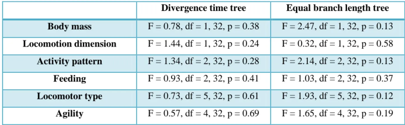
There is no significant correlation between FCL relative size and bodymass (all p values >0.13). Agility categories do not separate species according to FCL relative sizes (all p values >0.19). The FCL relative size does not vary with locomotion dimension (all p values >0.24) and locomotor type (all p values >0.12). The results remained unaltered when “fossorial” category (which had only 2 specimens) was removed from the analysis. The analysis revealed no difference between activity pattern (p value >0.13) and feeding categories (p value >0.37). When “Diurnal/Nocturnal” category was removed from the analysis the results did not change. The analysis of scatterplots reveals considerable variability within each ecological category (Figures 3.2, 3.3, 3.4, 3.5, 3.6). See table 3.1 for analyses result details.

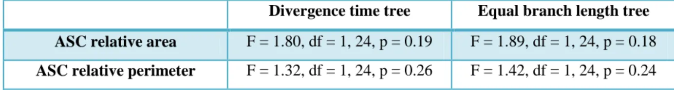
In what concerns the relative area of ASCs, I found no significant correlation with FCL relative size (p value>0.18, table 3.2, Figure 3.7). I also tested a correlation with ASCs perimeter, but it was also non-significant (table 3.2).

Table 3.1 – Results of the analyses of variance of the mammal data set. Statistics of the effect of each predictor on FCL relative size variation (F-test value, degrees of freedom and p value).

Divergence time tree Equal branch length tree Body mass F = 0.78, df = 1, 32, p = 0.38 F = 2.47, df = 1, 32, p = 0.13 Locomotion dimension F = 1.44, df = 1, 32, p = 0.24 F = 0.32, df = 1, 32, p = 0.58 Activity pattern F = 1.34, df = 2, 32, p = 0.28 F = 2.14, df = 2, 32, p = 0.13 Feeding F = 0.93, df = 2, 32, p = 0.41 F = 1.03, df = 2, 32, p = 0.37 Locomotor type F = 0.73, df = 5, 32, p = 0.61 F = 1.93, df = 5, 32, p = 0.12 Agility F = 0.57, df = 4, 32, p = 0.69 F = 1.65, df = 4, 32, p = 0.19

30

Table 3.2 - Results of the analyses of variance of the mammal data set. Statistics of the effect of ASC relative area and perimeter on FCL relative size variation (F-test value, degrees of freedom and p value).

Birds

The specimen with the largest optic lobes absolute volume is the Struthio camelus (ostrich) with 2585.47 mm3, while Selasphorus rufus (rufus hummingbird) had the smallest volume (17.60 mm3). Proportionally, Hirundo rustica (barn swallow) had the largest optic lobes relative size (15.54%) and the smallest value is observed in Strigops habroptila (0.34%). Phaethon lepturus (white-tailed tropicbird) has the largest relative optic lobes value and Tyto alba (barn owl) has the smallest, according to the residuals from an ordinary least-squares regression (see Materials and Methods).

Our analysis on bird data revealed no significant correlation between FCL relative size and body mass (all p values >0.31). The analysis of variance showed a difference in average relative size of nocturnal and diurnal birds (all p values <0.03) and feeding categories (all p values >0.02) (Figures 3.8, 3.9). When OL relative size was added to the analysis, no significant correlation with between FCL was obtained when using the divergence times tree (p = 0.16) but the equal branch tree returned a marginally significant result (p = 0.04) (see table 3.3).

Table 3.3 - Results of the analyses of variance of the bird data set. Statistics of the effect of each predictor on FCL relative size variation (F-test value, degrees of freedom and p value).

Divergence time tree Equal branch length tree Body mass F = 2.22, df = 1, 54, p = 0.14 F = 2.81, df = 1, 54, p = 0.09

Feeding F = 4.69, df = 2, 54, p = 0.01 F = 4.07, df = 2, 54, p = 0.02 Activity pattern F = 7.81, df = 1, 54, p < 0.01 F = 8.98, df = 1, 54, p < 0.01 Optic Lobes F = 2.02, df = 1, 51, p = 0.16 F = 4.32, df = 1, 51, p = 0.04

In sum, FCL relative size differs from feeding and activity pattern categories in birds. In mammals, no significant result was yielded for ecological categories. Both in mammals and birds, FCL relative size does not correlate with body mass.

Divergence time tree Equal branch length tree ASC relative area F = 1.80, df = 1, 24, p = 0.19 F = 1.89, df = 1, 24, p = 0.18 ASC relative perimeter F = 1.32, df = 1, 24, p = 0.26 F = 1.42, df = 1, 24, p = 0.24

31

Figure 3.1 – Mammals data scatterplot set with x = log10 body mass and y = FCL relative size. The blue line is an ordinary least-squares regression line and the grey area is the 95% confidence interval. Note six severe outliers in the bottom.

Figure 3.2 – Mammals data scatterplot set with x = feeding ecology and y = FCL relative size (residuals). For each category, error bars are presented. Both categories have some severe outliers like Procavia capensis (Gatherer), Paradoxurus sp. and Vulpes vulpes (Occasional predator), Puma concolor, Felis catus and

32

Figure 3.3 – Scatterplot of the mammals data set with x = locomotor type and y = FCL relative size (residuals). For each category, error bars are presented. Note the variability of Arboreal, Terrestrial and Scansorial

categories.

Figure 3.4 – Scatterplot of the mammals data set with x = locomotion dimension and y = FCL relative size (residuals). Note the variability within the 2D category.

33

Figure 3.5 – Scatterplot of the mammals data set with x = agility and y = FCL relative size (residuals). For each category, error bars are presented. Note the outlier in the Very Slow category, Procavia capensis. Medium category present highly variable values.

Figure 3.6 – Mammals data Scatterplot of the set with x = circadian activity pattern and y = FCL relative size (residuals). Values in all categories are highly variable.

34

Figure 3.7 – Mammals data scatterplot set with x = anterior semicircular canal relative area and y = FCL relative size. The blue line is an ordinary least-squares regression line and the grey area is the 95% confidence interval. The most severe outlier, in the bottom, is Procavia capensis.

Figure 3.8 – Birds data scatterplot of the set with x = circadian activity pattern and y = FCL relative size. The Diurnal category has variable values. Tyrannus tyrannus and Ara macao are severe outliers in the Diurnal group.