Gonçalo Morgado
152109078
Dissertation submitted in partial fulfillment of requirements for the degree of Masters of Science in Economics, at the Universidade Católica Portuguesa, December 2011
Dedicated To my parents, for all their love. For everything. And Girlfriend.
Abstract
Valuation is as important as difficult and is far from being an exact science. The aim of this dissertation is to analyze EDP – Energias de Portugal, SA under the theories and works of many authors that give all their work to develop the best techniques and assumptions to came up with the best valuation possible. Still, the debate will continue and many other opinions will appear.
Group EDP is enormous. Hence, this dissertation focuses on the most important business segment: Electrical business in Portugal and Spain. This work is done meanwhile Portugal is under financial intervention and it will affect directly EDP as it will be totally private.
The final objective is to compare my work with Caixa Banco de Investimento in their report of December 2010.
Table of Contents
I – LITERATURE REVIEW ... 7
1. INTRODUCTION... 7
1.1 WHAT IS VALUATION?... 7
1.2. DIFFERENT VALUATION METHODS – GENERAL REVIEW... 8
2. VALUATION METHODS... 11
2.1 RELATIVE VALUATION -‐ MULTIPLES... 11
2.2 DISCOUNTED CASH FLOW (DFC) METHODS... 15
2.2.1 WEIGHTED AVERAGE COST OF CAPITAL (WACC) -‐ IN DETAIL... 16
2.2.2 TAX SHIELDS... 17
2.2.3 ADJUSTED PRESENT VALUE (APV) ... 19
2.3 EQUITY CASH FLOWS (ECF) – FCFE... 20
2.4 OPTION VALUATION... 20
3. RISK FACTOR... 22
3.1 RISKFREE RATE... 22
3.2 BETAS -‐ Β... 24
3.3 EQUITY RISK PREMIUM (ERP)... 25
4. GROWTH RATES... 26
4.1 ESTIMATING GROWTH... 26
4.2 TERMINAL VALUE... 27
5. CROSS BORDER VALUATION... 27
6. CONCLUSION... 30
II – COMPANY ANALYSIS AND INDUSTRY REVIEW ... 30
1. PORTUGUESE AND SPANISH MACROECONOMIC ENVIRONMENTS... 31
1.1 PORTUGUESE MACROECONOMIC SCENARIO... 31
1.2. PORTUGAL: MEMORANDUM OF UNDERSTANDING ON SPECIFIC ECONOMIC POLICY CONDITIONALITY – ELECTRICAL MARKET. ... 32
1.3 SPANISH MACROECONOMIC SCENARIO... 33
2. PORTUGUESE ELECTRICAL MARKET – MARKET SHARES BY SECTOR. ... 34
3. SPAIN – MARKET ANALYSIS... 38
3.1 PREVIOUS YEAR DEMAND REVIEW... 38
3.2 SPANISH ELECTRICAL INDUSTRY DEFICITS AND CHALLENGES... 38
4. CAPEX AND ROCE PERSPECTIVES... 39
5. INDUSTRY DEBT LEVELS – A CONCERN... 41
6. COMPARING IBERIAN COMPANIES PERFORMANCE WITH THEIR EUROPEAN PEERS... 41
7. COMPANY ANALYSIS... 42
7.1 EDP – ACTIVITY FIGURES... 42
7.2 EDP INSTALLED CAPACITY AND KEY FACTORS... 44
7.3 EMISSIONS TRADING... 46
7.4 EDP CAPITAL STRUCTURE AND MARKET PERFORMANCE... 46
7.5 COMPANY BUSINESSES STRUCTURE... 49
7.6 COMPETITORS... 50
III – VALUATION... 51
1. INVESTMENT CASE... 51
2. METHODOLOGY... 53
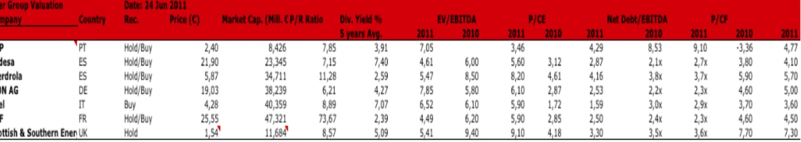
2.1. PEER GROUP CONSIDERATIONS... 54
4. DATA... 56
4.1. GROWTH RATE... 56
4.2. COST STRUCTURE AND OTHER REVENUES DATA... 57
4.3. DATA ASSUMPTIONS... 58
4.4. EDP RATING... 60
5. DIVIDEND POLICY... 60
6. FINANCIAL RATIOS FORECAST... 61
7. EDP PROFIT & LOSSES STATEMENTS PER AREA: PRODUCTION, DISTRIBUTION AND COMMERCIALIZATION ... 63 8. DEBT... 63 9. MULTIPLES VALUATION... 64 10. GAS VALUATION... 65 11. DCF VALUATION... 65 11.1 TANGIBLE ASSETS... 65 11.2. INTANGIBLE ASSETS... 66
11.3. INVENTORY, CLIENTS, TRADE DEBTORS, CURRENT ASSETS, TRADE CREDITORS AND OTHER CREDITORS ... 66
11.4 NET WORKING CAPITAL... 67
11.5 CAPEX ... 68
13. SUM-‐OF-‐PARTS VALUATION... 69
14. COMPARISON WITH CAIXA INVESTMENT BANK REPORT... 70
ANNEXES ... 74
A. NATURAL MONOPOLY... 74
B. MIBEL AND OMIP... 74
B.1 MIBEL – MERCADO IBÉRICO DE ELECTRICIDADE -‐ IN DETAIL... 74
B.2 OMIP -‐ PRACTICAL PART OF MIBEL ... 76
C. EDP SWAT ANALYSIS... 78
1. EDP FINANCIAL STATEMENTS – HISTORICAL RESUME... 79
3. COUNTRY RISK PREMIUM... 80
4. CAPITAL STRUCTURE TARGET... 81
5. EDP RATINGS... 81
5.1. MOODY’S RATINGS... 81
6. EDP IBERIAN PRODUCTION P&L ... 82
7. EDP IBERIAN DISTRIBUTION P&L ... 83
8. EDP IBERIAN COMMERCIALIZATION P&L ... 84
9. EDP IBERIAN CONSOLIDATED P&L AND BALANCE SHEET... 85
10. DEBT... 87
10.1 DEBT PER CURRENCIES... 88
10.2 DEBT MARKET VALUE... 89
11. GAS P&L ... 90
12. TANGIBLE ASSETS... 91
13. INTANGIBLE ASSETS... 91
14. INVENTORY, CLIENTS, TRADE DEBTORS, OTHER TRADE DEBTORS, OTHER CURRENT ASSETS AND TRADE CREDITORS AND OTHER CREDITORS... 92
15. NET WORKING CAPITAL... 92
16. CAPEX ... 92
17. EDP FINANCIAL INVESTMENTS... 92
17.1 EDP RENOVÁVEIS... 92
17.3. BCP ... 93
18. COMPARISON WITH CAIXA BI – BANCO DE INVESTIMENTO... 94 BIBLIOGRAPHY... 95
I – Literature Review
1. Introduction1.1 What is Valuation?
“Every asset, financial as well as real, has a value” (Damodaran, 2002). Knowing that, the point is how and when to measure it. There are plenty of options to do it. Somehow, there are some saturation of different methods, so it is fundamental to choose the best one giving the different assets as “managing assets lies in understanding not only what the value is but also the sources of the value” (Damodaran, 2002).
Valuation is an Art. It is a tough job to do it giving that there are some ideas that do not correspond to the truth. Damodaran (2002) points out some “Myths” that must be taken into consideration. The first one is that “Since Valuation Models are quantitative, valuation is objective” (Damodaran, 2002). The true behind this myth is that, a correct valuation is somehow in the middle of a strong quantitative evaluation but also taking into account several points that are not pure “sum-‐of-‐ parts”. All businesses and companies are different, even though sharing some characteristics that an Analyst can exploit to come up with better evaluations. A simple example is that, evaluate a Mature company is not the same as evaluate a start up, not only because of their cash flows but also because one can be in a stable market and the other in a turmoil situation. It is easy to understand that only by looking at different Equity Research from different Investment companies. Evaluation is also a question of beliefs in the future and since future is unpredictable, people may analyse it in a different way, hence, different values will come up.
“When the facts change, I change my mind. And what do you do, sir?” – Lord Keynes (Damodaran, 2002). This sentence explains other myth that Damodaran stresses: “A well-‐research and well-‐done valuation is timeless”. Everything changes, even more in the economy, so all the assumption that analysts take to evaluate one company can change quickly so; they must be aware of that and change it on a regular basis in order to have credible final value. The author continue to point other myths such as “A good valuation provides a precise estimate of value” or that “the more quantitative a model, the better the valuation” (Damodaran, 2002) among
others that are not important to focus now for the rest of the work, but to remember meanwhile analysts develop their evaluations.
1.2. Different Valuation Methods – General Review
Source: Pablo Fernandéz, Company Valuation Methods, 2002.
As mentioned above, there are plenty of options to do a company valuation, and Fernandéz (2002) summarizes it quite well in the table above. There are several ways to evaluate and all of them will come up with different values as all of them start and focus on different assumptions – the price is not the point, the value is. “A company’s value is different for different buyers and it may also be different for the buyer and the seller” (Fernandéz, 2002). Not surprisingly, it is of extreme importance to understand whether there is some manipulation or not of the different methods.
Fernandéz (2002) develop an extensive explanation whether one method is better than other knowing that people may prefer different ones. The purpose of this work is not to describe each one of them but to have a brief idea of all the option and the reason why to focus on a specific one.
Starting with the balance sheet methodology we have that some valuations can be made through the observation of the balance sheet forgetting future opportunities, only looking to the “year photo” of the company. Inside this method we have the Adjusted Book Value and “this method seeks to overcome the shortcomings that appear when purely accounting criteria are applied in the valuation” (Fernandéz, 2002). The aim here is to match book values with market values.
The second valuation option mentioned by Fernandéz, P. (See table above) is the income statement-‐based methods which “seek to determine the company’s value through the size of its earnings, sales and other indicators” (Fernandéz, 2002) commonly known as Multiples that are one of the most important evaluation methods and will be deeply analyze afterwards given their importance and appliance to any valuation. The third one, Mixed (Goodwill) – “Goodwill is the value that a company has above its book value or above Adjusted Book Value. (…) Seeks to represent the value of the company’s intangible assets (…), contribute an advantage with respect to other companies operating in the industry” (Fernandéz, 2002)
The 4th given method, Cash flow Discount, is the most important one. Any credible valuation must have it and this work will focus on it this method, as well as with the Multiples. It is a very well known method and its likely to be the only one that can be assumed to base final decisions. Fernandéz (2002) summarizes it as all other authors as “this method seeks to determine the company’s value by estimating the cash flows it will generate in the future and discounting them at the discount rate matched to the flow’s risk” (2002).
Still, it is important to clarify the statement “discount rate matched to the flow’s risk” and it can be summarized in the table below.
Source: Fernandéz, P. “Company Valuation Methods” (2002)
A company valuation can be made from different perspectives; generally speaking, it can be whether focusing on free cash flow from operations or from equity cash flows. Giving that, we must be aware that they have different risks, so they must be discounted at different discounts rate.
The fifth method, value creation is more used to evaluate some projects inside the company, as they are easy to compute and directly compare the return and associated risk.
Finally, Options valuation is very useful to do valuations when dealing with commodities traded in the market or investment opportunities whether to develop or stop. Hence, companies with high exposure to this kind of assets must consider this valuation tool as a good option.
After this brief introduction about all available methods to do companies valuation according to the actual state of art, Fernandéz (2002) presents a table from Morgan Stanley that put it clear that the PER is the most widely used method – See table below. The reason behind it might be that it is an easy method to compute and get the information as well as simple to compare between two companies. All the others are more complex and require more assumption mainly – again – DCF methods.
Source: Morgan Stanley Dean witter Research – Paper: Fernandéz, P. – Valuation using multiples, 2001.
Fernandéz (2001) states that “Multiples are useful in a second stage of valuation: After performing the valuation using another method, a comparison with the multiples of comparable firms enable us to gauge the valuation performed and identify differences between the firm valued and the firms it is compared with”.
0% 10% 20% 30% 40% 50% 60%
PER to growth EV/FCF EV/Sales FCF DCF Residual Income PER
Percentage of Analysts that use each
method
2. Valuation Methods
2.1 Relative Valuation -‐ Multiples
Multiples are widely used as confirmed before. They are a rich and useful valuation method. “The valuation principle behind Multiples is the relative valuation” as Damodaran, A. (2006) points out – “In relative valuation we value an asset based upon how similar assets are priced in the market” (Damodaran, 2006). In relative valuation we can compare everything, the big problem is what can be compare exactly. Compare two different companies, even though, they are in the same industry is much harder and easy to make mistakes. All companies are different, no matter if in terms of business or in their financial statements and that affect decisively the conclusions and efficiency of the Multiples doing valuations. Damodaran, A. (2006) put it clear comparing with the DCF methods in a simple way: “In discounting cash flows, we are attempting to estimate the intrinsic value of an asset based upon its capacity to generate cash flows in the future. In relative valuation, (…) making a judgement on how much an asset is worth by looking at what the market is paying for similar assets”. Still, Damodaran, A. (2006) points one common factor between these two methods: “Every Multiple, (…), is a function of the same three variables – Risk, Growth and cash flow generating potential” as well as DCF assumptions. In line with this finding, other authors find that “Investment banks and appraisers regularly use valuation by multiples, such as P/E multiple, instead of or as a supplement to DCF analysis” (Lie and Lie, 2002).
Damodaran, A. (2006) distinguishes Multiples into three major groups: Earnings, Revenues and Book Value. Moreover, Damodaran, A. (2006) and other authors stresses the fact of what is a “comparable firm”, the main difficulty to correctly use Multiples. Damodaran (2006) defines it, as “one with cash flows, growth potential, and risk are similar to this firm being valued”. Goedhart et al. (2005) make it clear: “Multiples are often misunderstood and, even more often, misapplied. (…) The use of the Industry average (…) overlooks the fact that companies, even in the same Industry can have drastically different expected growth rates, return on invested capital and capital structure”. Goedhart et al. (2005) suggest that the way to do that is by “matching those (companies) with similar expectations for growth and ROIC”.
Goedhart et al, (2005) goes more into detail in where he defines as a “well-‐tempered Multiples”. The author states that the best way to avoid errors that can put in stake the valuation results are:
i. Use peer with similar prospects for ROIC and growth; ii. Use forward-‐looking multiples
iii. Use enterprise-‐value multiples;
iv. Adjust the Enterprise-‐value-‐to-‐EBITA multiple for non-‐operating items.
It is important to notice that is possible to end up with only one “comparable” firm. However, Andreas Schreiner (2007) argues, “If we end up with fewer than two peers, we must either ease the restrictions or use another valuation method. If we have more than two peers, an examination of financial ratios and multiples of the remaining follow”. Adding to that, when computing the multiples it is fundamental to have high sensitivity to the specific business and Goedhart et al. (2005) consider it as the difference between “sophisticated veterans from newcomers”. In the second point, Goedhart (2005) find with evidence that there is lower dispersion comparing forward-‐looking multiples than with historical data. This point agrees with the findings of Lie and Lie (2002) where they find out “that the P/E multiple based on forecast earnings provides more accurate estimates than the P/E based on historical earnings” (Lie and Lie, 2002). Third, the opinion that we should use enterprise-‐value multiples come up from the two flaws of the P/E multiples. First, “systematically affected by capital structure” (Goedhart et al., 2005) and, second, “P/E ratio is based on earning, which include many non-‐operating items”. Hence, his “alternative to the P/E ratio is the ratio of enterprise value to EBITA. (…) Is less susceptible to manipulation by changes in capital structure” (Goedhart et al., 2005). Finally, the author finds it essential to adjust the Enterprise-‐value-‐EBITA multiple for non-‐ operating items because, otherwise, we will be generating “misleading results” (Goedhart et al., 2005).
Lie and Lie (2002) states that “a direct comparison of the multiples that provide estimates of Equity value versus those that provide estimates of total
enterprise value may not be entirely fair but (…) provide valuable insights”. Their three main findings are interesting in this point of the study:
i. Forecasted against historical values. Same conclusion as Goedhart et al. (2005)
ii. Adjusting for the cash levels has an ambiguous and marginal effect on valuation accuracy. Here, we have same discussion when comparing the two authors, Goedhart (2005) and Lie and Lie (2002).
iii. Of the total enterprise value multiples the asset multiple provides the most accurate and the sales multiples the least accurate estimate. (Lie and Lie, 2002)
Table: Fundamentals determining Equity Multiples.
Source: Damodaran, A. Valuation Approaches and Metrics, 2006.
A clear common factor in the table above is the expected growth rate. Still, even in the same industry companies can be in different growth stages and that affect their cash flows.
According to Fernandéz (2001) the most widely used Multiples are: PER and EV/EBITDA. However, he notices that depending on the Industry some Multiples may have more relevance than others. To confirm, separate different industries and checked which multiples are more useful.
PER = Market Capitalization / Total Net Income = Share Price / Earning per share (Price Earning Ratio)
P/CE = Market Capitalization / (net income before depreciation and Amortization) (Price to Cash Offering)
Source: Fernandéz, P. Valuation using multiples. 2001
Again, according to Fernandéz, P. (2001), similarly with Damodaran (2006), divides the multiples into three groups:
i. Multiples based on the company capitalization (Equity Value: E) ii. Multiples based on company’s value (Equity and Debt value: E+D) iii. Growth reference multiples.
However, Fernandéz (2001), points out that multiples show high dispersion and the PER, the most used one is also the one with higher dispersion. The table below represents the average volatility of several parameters used for multiples.
Source: Fernandéz, P. Valuation using Multiples. How do analysts reach their conclusions, 2001. Multiples of 26 Spanish companies between 1991-‐1999.
Fernandéz (2001) presents that multiples are useful and important but face some important limitations, where the first one, is their dispersion and that may affect brokers decisions.
Adding to “dispersion” Lie and Lie (2002) found that “valuations are more accurate for large companies”. The second conclusion is clear: “large companies are undervalue”. Third, no matter company size, “the asset multiple yielded the most accurate assessments whereas the earning-‐based multiples yielded the least accurate” and, finally, “a combination of multiples perform better than individual multiples. (…) Companies with high earnings, earnings-‐based multiples produce
positive valuation biases whereas the asset multiples yield negative biases”. (Lie and Lie, 2002).
Andreas Schreiner (2007) concludes, in line with other authors, the strengths and weaknesses of Multiples (See Table)
Strengths and Weaknesses of the Standard Multiples methods
Source: Andreas Schreiner, Equity valuation using Multiples, 2007
2.2 Discounted Cash Flow (DFC) Methods
“Value – measured in terms of discounted cash flows – is the best metric for company performance that we know” (Thomas E. Copeland, 1994)
Discounted Cash Flow (DCF) is the best method to evaluate a company, and it is impossible to run a firm valuation without considering it. Among other reasons, because cash flows are believed to be less susceptible to manipulation as some accounting standards (Juliet Estridge and Barbara Lougee, 2007). Cash Flows are kings in valuation. In fact, there are several methods to do valuation but also when considering DCF there are some different approaches. Fernandéz, P. (2002) considers 10 methods from 9 theories. The most important conclusion is that results should be the same as all of them evaluate the same reality under the same assumptions (Fernandéz, 2002). Jacob Oded and Allen Michel (2007) summarize in four methods as well as Cooper and Nyborg (2006). And they are:
i. Adjusted Present Value (APV) ii. Capital Cash Flow (CCF)
iii. Equity Cash Flow (ECF) iv. Firm Cash Flow (FCF)
There is consensus here, the discussion is that, when to use each method. In the case, and according to literature, the more appropriate is Discounting the free cash flow with WACC (Cooper and Nyborg, 2006). These two authors defend existing literature and explore the well-‐known theory of Modigliani-‐Miller and Milles-‐Ezzell. The way to run valuations is by discounting future cash flows – nothing new here – but with which discount rate? WACC appear to be the best one as combines the Kd and Ke, depending on the specific weight of Equity and Debt. Moreover, it should be After-‐Tax, in order to get the tax shields. According to literature the problem remains how to evaluate the Tax shields, as literature dos not give an exact method. All the rest are, more or less, well explained in the actual state of art. Finally, Jacob Oded and Allen Michel (2007) argue that it is possible to reconcile all DCF methods and they will have all the “unique value” of the firm. The authors criticize the fact that the choice of each method depends on the debt rebalancing. In their opinion, it is not necessary, as all methods should lead to the same firm value even if companies change their debt.
2.2.1 Weighted Average Cost of Capital (WACC) -‐ in detail
The traditional approach of WACC is well known and it is as follow:
WACC = Rd (1-‐T)(D/V) + Re (E/V)
Although not common, Ross, Westerfield and Jordan (2006) recall the fact that we should add to the WACC formula Rp1. (P2/V) whenever we are valuing a company
with preferred stock as financing source.
WACC is fundamental to run any valuation through DCF. It is the required rate of return on the overall firm (Ross, Westerfield and Jordan, 2006). The criticism about the formula is because of their assumptions. Ramiz ur Rehman and Awais Raoof (2010) summarize it:
i. All Dividends should be paid out as dividends
1 Cost of Preferred Stock 2 Value of the Preferred Stock
ii. Growth rate will be zero
iii. Market value of Debt is equal to book value
According to the literature, it is more accurate to value a company through the sum of the PV of debt and the PV of Equity at their specific discount rate, Rd and Re, respectively (Fernando Llano-‐Ferro, 2009). Rehman and Raoof (2010) although points out some criticisms about the paper of Llano-‐Ferro (2009) even though agree with the fact that the alternative approach to get the WACC is more accurate and provide better results.
2.2.2 Tax Shields
When considering the value of the tax shields (VTS), literature is not conclusive. Hardly we get a clear way to calculate it even though such an important value to consider when valuing companies. In a perfect scenario there are no taxes so it is indifferent whether to use or not debt (Modigliani-‐Miller, 1963). Still, real world is much more complex and there are taxes and other external costs, such as bankruptcy costs. Giving that, companies to maximize value use different debt strategies whether by using fixed target debt ratios or adapting it frequently. As it depends on many factors, literature does not provide a clear answer, it leaves on the decision of who is performing a valuation (Copeland, Koller and Murrin, 2000, Fernandéz, 2002). The following table summarizes the different perspectives of different authors, considering the Value of Tax Shields (VTS) in perpetuities.
Source: Fernandéz, P., 2002. Table 1. Comparison of the VTS in Perpetuities3
3 VTS = Value of the tax shields; Ku = Unlevered cost of Equity; Kd = required return
on debt; T = Corporate tax rate; D = Debt Value; Rf = Riskfree rate; PV (Ku; D T Ku) = Present value of D T Ku discounted at the rate Ku.
Even though there is some discussion on how should be calculate the tax shields, some authors must be taken into consideration more carefully, such as Fernandéz (2002) and Ian A. Cooper and Kjell G. Nyborg (2005) that contradicts the first one, defending past authors and existing literature.
The first one to consider is Fernandéz (2002) that come up with a new way to calculate the tax shields going against some existing literature normally accepted. His point is clear: Tax savings should not be thinking as the Present Value (PV) of a cash flow, but the difference between the cash flows of an unlevered company with a levered one (Fernandéz, 2002). The author also adds “”discounting value of tax shields” in itself is senseless” (2002). The way he sees it is as: VTS = Gu4 – Gl5. It is
this difference that gives us the VTS that increases company’s value and not the PV of tax shields due to interest payments (Fernandéz, 2002) and that leads us, to a well know formula: VTS = D.T. Even though it is not a new idea in the specific literature the author derives it in a different way as previous literature add an “α” (Fernandéz, 2002). For this specific α, Modigliani-‐Miller (1963) suggests the Rf6 and Myers (1974)
the Kd7. Fernandéz (2002) maintain it simple and, in this specific case of perpetuities,
the author concludes, again, “the value of tax shields is the difference between Gu and Gl, which are the present values of the two cash flows with different risks: The taxes paid by the unlevered company and the taxes paid by the levered company” (Fernandéz, 2002).
In his paper, Fernandéz, P. (2002) agrees that the VTS should be calculated differently depending on company’s debt strategy. If the strategy is to have a fixed debt target (D/(D+E)), according to Milles-‐Ezzell (1980) the first year should be discounted at Kd and the rest with Ku8. On the other hand, if the company has a
more flexible debt target, it should be calculated according to Myers (1974).
In the opposite way, Cooper and Nyborg (2005) defend the existing literature by pointing out some results that are not correct under Fernandéz (2002) theory.
4 PV of the taxes paid by the unlevered company 5 PV of the taxes paid by the levered company 6 Risk-‐free rate
7 Cost of Debt
The main conclusion is simply that “the value of debt tax saving is the present value of the tax savings from interest” (Cooper and Nyborg, 2005). What they criticize in Fernandéz (2002) is that he mixed Miles and Ezzell and Modigliani-‐Miller framework. Moreover, Fernandéz (2002) used some assumptions that must be proved and not only assumed, such as Ke9 that does not grow even though we have a g10 > 0. Adding to that, Fernandéz (2002) is supposed to be working in a standard Milles-‐Ezzell (1980) framework but with “an alternative interpretation” (Cooper and Nyborg, 2005). The author works with a constant leverage ratio, thus, his assumption of VTS = DT is not correct, as the tax shield is risky. The authors also critic that “if the discount rate for the cash flows is a constant that is independent of growth, Fernandéz’s assumptions are internally inconsistent” (2005)
To conclude, its clear that there are no consensus in this field, that Fernandéz (2002) presented a good idea to calculate the VTS but he made few mistakes according to Cooper and Nyborg (2005) that defend the existing theory. Thus, and also regarding those other authors, as mentioned above, leave to the preference of each reader to decide, it is more coherent to focus on the existing literature in spite of adapt to a new theory that, per se, is not conclusive.
2.2.3 Adjusted Present Value (APV)
“APV always work when WACC11 does, and sometimes when WACC
doesn’t because it requires fewer restrictive assumptions” (Luehrman, 1997) First of all, APV is also a DCF method. However, the idea that WACC is obsolete and only a standard method gave to APV the belief that this new method is more “transparent” (Luehrman, 1997). Another similar characteristic is that APV is useful to value operations and assets-‐in-‐place. The main difference to mention is that APV relies on value adding by splitting the problem in as much as possible different situations. The method general formula is as follow:
APV = Base Case Value + Value of all financing side effects.
9 Cost of Equity 10 Growth rate
In the base case it is considered the value of the unlevered company all Equity financed. Therefore, the discount factor will be the Ke12. From financing side effects it is considered parts such as interest tax shields, costs of financial distress, subsidies among others. The discount factor should reflect only time value and riskiness of the project (Luehrman, 1997). When comparing with WACC that gather everything in the same model, here we have to focus on all separate parts and, finally, sum them all. To conclude, APV is an interesting method, believe to be the best one and is substituting the WACC that all people are used to. The reason behind that is because its simpler and separate operations that as consequence, provide better information to take decision and understand exactly from where value is being created.
2.3 Equity Cash Flows (ECF) – FCFE
Luehrman (1997) believe that it is a more specific method and it is important as a third possible method. The support of this method is that sometimes it is worth to accept projects with negative NPV. Moreover, when considering companies with high leverage and in business trouble, shareholders can act as if they own an Option. This means, if equity gains are high enough, they will exercise it, otherwise, they do not and left the company to debtholders (Luehrman, 1997). This method are good to know how shareholders are being remunerated and if they are satisfied or not. ECF is a good method to do financial institutions (Banks and Insurance) valuation. It is not the case hence this point will not be further developed.
2.4 Option Valuation
Literature finds it more useful than ever. It presents a variety of opportunities for business decision makers, however, some problems for those who want to do valuation considering it. First of all, Options can be used with success in every Industry. In the case, we are evaluating an electric company; several benefits can be exploit from their use. Thomas E. Copeland and Philip T. Keenan (1998) summarizes it as follows:
Source: Thomas E. Copeland and Philip T. Keenan, Making Real Options Real, 1998.
By revising the literature about the usefulness of Option valuation it is possible to find that all the authors agree that Option Valuation is an important complement to DCF methods, but not a complete substitute. A common thing they present in their papers: DCF undervalues Investment opportunities. (Simon Wooley and Fabio Cannizzo, 2005). In the same line, Thomas E. Copeland and Philip T. Keenan (1998) points that the exclusive use of “Net Present Value (NPV) and Economic Profit have been responsible for systematic underinvestment and stagnation” (1998).
The main advantage of using real option valuation is Flexibility. Moreover, when we are considering assets traded in the market and long-‐term investment periods. “In the long-‐run, commodity prices tend to revert to fundamental levels, a characteristic know as “mean reversion” (Simon Wooley and Fabio Cannizzo, 2005), hence, the use of Black-‐Scholes tend to overvalue long term options. In order to avoid that, the authors found as solution the use of the same discount rate as in the DCF method and not the Riskfree rate as previous authors believed. Finally, these two author conclude that, if in one hand, an increase in the volatility of the project increase their value, on the other hand, an increase in the rate of the mean reversion leads to a reduction in the project value (2005). Tom Arnold (2004) shows that using risk-‐adjusted discount rates produces a real option valuation identical to that obtained from a risk-‐neutral option valuation, this means that, NPV and risk neutral option valuation are equivalent.
Considering an Electric utility (as It is the case) the importance of options valuation is to do some “pecking order” of the different possibilities to produce energy whether it should be done, at a certain moment in time, by coal, gas, nuclear plants or renewable sources. All the different possibilities, face different prices in the markets so, by using option contracts, the Electric Company can do some kind of “pecking order” with their resources in order to maximize their profits over time.
Moreover, the decision of construct a new central will depend on the value of the resources in the market. All these decisions can be based in options valuation. Thomas E. Copeland and Philip T. Keenan (1998) separate these options in two groups:
1. Compound Options: When exercised gives the option to enter in a new option (continue investing in a new investment)
2. Learning Options: Learn about the uncertainty (Prices volatility in the market) Still, the authors conclude that, the value of each option is more valuable than the sum of each one of them. Adding to that, they found it extremely useful in Cyclical Industries (as EDP with different demand in the summer and winter) that must decide over time the use of different factories or supply contracts. Again, an option contract is only useful whenever the information can modify future investment decision (Thomas E. Copeland and Philip T. Keenan, 1998)
However, Option valuation presents a considerable problem. They are hard to analyse and, most times, only the top managers are aware of them and can value. Outside people hardly know whether there exist or not, and even more difficult to understand what is its value. Concluding, authors found it extremely useful as a complement to DCF methods or other, but of difficult access for outside investors that are not in the decision-‐making.
3. Risk Factor
3.1 Riskfree Rate
Damodaran (2008) define the riskfree asset as: “An investment can be riskfree only if it is issued by an entity with no default risk, and the specific instrument used to derive the riskfree rate will vary depending upon the period over which you want the return to be guaranteed”
Usually, the Riskfree rate is simplified with looking at the rate of government bonds in a specific market and must have the two following characteristics:
i. No default risk
Considering the first point, automatically exclude corporate bonds because, even if it is an extremely stable and profitable company, it always copes with default risk. Hence, only government bonds can be considered as riskfree rates, but not always. The principle behind it is that the government print their currency, so, at least, in nominal terms the repayment is guaranteed (Damodaran, 2008). The riskfree rate is very important and the starting point of any valuation as it influences all other rates and, as consequence, will impact on the company value that can lead to lower company value. (Damodaran, 2008) That impact influence both Equity premium and Debt rate. The riskfree rate is the base and we only add the Equity premium or Spread -‐ the base of CAPM13. So, the higher the
riskfree, the higher will be both Equity premiums and Debt that will influence negatively the valuation of the company.
Another point to take into consideration when considering which riskfree rate we will use is the Duration. Damodaran (2008) think that, when comparing 10 or 30 years government bond rates, should be used the 10-‐year bond rate to discount cash flows, at least in mature markets. (Damodaran, 2008) After that, Damodaran focus the point that, the choice of the riskfree rate must be considering the country’s currency. In his paper (2008) he notices the specific case of Europe that, even though all government trade their bonds in Euros, they all have different rates, as investors are aware that the capacity to repay the bonds differs considerably. Consequently, Damodaran (2008) believes that in Europe the different countries face some default risk, as they do not control their currency. Giving that, 10-‐years German bonds are assumed as the riskfree rate in the European market (And this Equity Research will have it as Riskfree rate too).
Finally, riskfree rate must be in real terms instead of nominal, in order to know the real return. Moreover, the riskfree rate is highly influenced by the inflation, so the lower it is, the lower it will be the riskfree rate (Damodaran, 2008).
3.2 Betas -‐ β
Betas (β) represent the systematic risk that cannot be eliminated by diversification (Barr Rosenberg and James Guy, 1995). It affects all Industries even though in different levels depending on the Industry volatility and market impact on their results. As characteristics Damodaran, A. (1996) defines it more generally as:
i. Risk Added on to a diversified Portfolio; ii. Measure the relative risk.
Barr Rosenberg and James Guy (1995) identify the use of Betas for three different purposes:
i. Performance valuation; ii. Investment Strategy;
iii. Valuation: “The higher the underlying risk, the more likely the security price change (…) Knowledge the value of Beta permits prediction of one important element of risk”
Continue with the same authors they believe that Beta vary between 0 and 3 but also “recall that we never observe the “true” Beta but rather outcomes that are randomly distributed about an expected value” (1995).
According to Damodaran (1996) when considering Betas some points must be considered. First of all, the more securities an Index has, the better it is. Secondly, it is important to consider a time horizon relatively large in order to get better results even though companies change that may affect the true values. Finally, choose the return interval. If it is too long, it decreases the number of observations that, consequently, will lead to lower correlations.
Other authors considered in this specific point, Paul D. Kaplan and James D. Peterson (1998) prove that when considering the Beta should be from the same Industry, what they call “Pure Plays Portfolio” (1998). It is extremely difficult to get companies that are 100% in the same Industry. But only when considering it, we have the better outcomes. Additionally, they found out that conglomerates and companies with high market capitalization tend to have lower betas than small companies.
To conclude, beta is fundamental to get information about the Industries that are being evaluated. Moreover, as it defines Industry and are affected by the economic environment, the higher the beta in one Industry, the higher company’s returns will fluctuate. Electric companies are expected to have values approximate or lower than 1, this means, follow the market movements in a slower level.
Source: Damodaran, A. Data base, Betas By Industy
3.3 Equity Risk Premium (ERP)
“Equity risk Premium is a key component of every valuation” (Damodaran, A., 2008). And it is generally defined as the difference between the risky security return and the risk free security. However, it is still a narrow subject as its values depend on different perceptions of the market by the different players. It is a fundamental part to assess the risks of the Industry, company or asset, so a correct value is essential to run valuations. More generally, Damodaran (2008) considers the determinants of the Equity Risk Premium (ERP) as: Risk Aversion;
Economic Risk; Information; Liquidity; Catastrophic Risk; Behavioural/irrational component.
Fernandéz (2011) separate it into four parts:
• Historical Equity Premium: Easy to calculate and equal to all investors
• Expected Equity Premium: Investors and Academics have different expectations
• Required Equity Premium: Crucial parameter to determine both Equity return and WACC
• Implied Equity Premium: is the implicit REP used in the valuation of a Stock (or market index) that matches the current market prices. Still, it is no common for all investors.