Multiplier adjustment in data envelopment analysis

35

MULTIPLIER ADJUSTMENT IN DATA ENVELOPMENT ANALYSIS

Jorge Azevedo Santos (Universidade de Évora)

Luís Cavique Santos (Universidade Aberta)

Armando Brito Mendes (Universidade dos Açores).

Abstract – Weights restriction is a well-known tech-nique in the DEA field. When those techtech-niques are applied, weights cluster around its new limits, making its evaluation dependent of its levels. This paper introduces a new ap-proach to weights adjustment by Goal Programming tech-niques, avoiding the imposition of hard restrictions that can even lead to unfeasibility. This method results in mod-els that are more flexible.

Keywords: Data Envelopment Analysis, Efficiency, Weights Restriction, Evaluation, Goal Programming.

I. INTRODUCTION

Data Envelopment Analysis (DEA) is a mathemati-cal programming based technique to evaluate the rela-tive performance of organisations. While the main ap-plications have been in the evaluation of not-for-profit organisations, the technique can be successfully applied to other organisations, as a recent evaluation of banks in India has demonstrated [1].

With this paper, we have two objectives in mind. The first one is to present DEA-Data Envelopment Analysis, a technique which may have useful applications in many evaluation contexts, namely when assessing not-for-profit organisations. In addition to allowing the ranking of the organisations traditionally termed decision-making units, DEA also creates the conditions to im-prove performance through target setting and role-model identification. We also briefly describe the technique of deleted domain, also known as Superefficiency.

The second objective is to introduce an entirely new way of adjusting multipliers by means of Goal Pro-gramming Techniques. This adjustment is a much more general way of dealing with the incorporation of exoge-nous structure preferences so far relying only in weights restriction techniques, which, in our point of view leads to the concentration of the weights in its upper and lower limits.

DEA is suited for this type of evaluation because it enables results to be compared making allowances for factors [2]. DEA makes it possible to identify efficient and inefficient units in a framework where results are considered in their particular context. In addition, DEA also provides information that enables the comparison of each inefficient unit with its "peer group", that is to say,

a group of efficient units that are identical with the units under analysis. These role-model units can then be stud-ied in order to identify the success factors that other comparable units can attempt to follow. Thanassoulis et al [3] argue that DEA is preferable to other methods, such as regression analysis, which also make it possible to contextualize results.

The present paper is structured as follows. The next section describes the development and fields of applica-tion of the technique, while secapplica-tion III introduces the DEA models followed by a numerical example. In sec-tion IV, we present Superefficiency evaluasec-tion, an ex-tension of DEA also known as deleted domain. Section V and VI deal with the graphical solution in the weights space and makes a very short description of the weights restrictions technique respectively.

In section VII, a new concept of multiplier adjust-ment is introduced and exemplified through a small data set.

In section VIII, a case with artificially generated data is solved to highlight the potentialities of this technique. This paper ends up with a final section with the conclu-sions and directions of future work. Readership not familiar with DEA, may find the brief introduction to the method presented below useful, but for those who wish to follow the matter further there is a good review of DEA in Boussofiane et al [4].

II. HISTORY AND APPLICATIONS OF DEA DEA is a mathematical programming technique pre-sented in 1978 by Charnes, Cooper and Rhodes [5], although its roots may be found as early as 1957 in Far-rel`s seminal work [6]. This technique is usually intro-duced as a non-parametric one, but in fact, it rests on the assumption of linearity [7] and for the original models even in the more stringent assumption of proportional-ity.

Its application has been focused mainly on the effi-ciency assessment of not-for-profit organizations, since these cannot be evaluated on the basis of traditional economic and financial indicators used for commercial companies.

The first application of DEA was in the field of Edu-cation, in the analysis of the Program Follow Through, conducted in the USA, in the late seventies [8]. Since then, it has been used to assess efficiency in areas such as health [9, 10], prisons [11], courts [12], universities and many other not-for-profit sectors. Nowadays, DEA can be seen to have spread to other fields such as Transit [13], Mining [14], Air Transportation [15], and even Banking and Finance [16].

However, many applications belong to the field of education and range from primary education [17, 18], to secondary [19, 20, 21] and university levels [22].

In Data Envelopment Analysis, the organizational units to be assessed should be relatively homogeneous and were originally termed Decision Making Units. As the whole technique is based on, the comparison of each DMU with all the remaining ones a considerable large set of units is necessary for the assessment to be mean-ingful. We will assume that each DMU produces N outputs by means of M inputs.

III. DEA FORMULATIONS WITH A NUMERICAL EXAMPLE

In DEA, efficiency (hj’) of a specific decision mak-ing unit (DMU j’) is defined as the ratio between a weighted sum of its N outputs Ynj’ and a weighted sum of its M inputs Xmj’, a natural extension of the concept of efficiency used in the fields of physics and engineer-ing [23]:

∑

∑

= =

=

M m mj mj N n njnj

x

y

v

h

1 ' ' 1 ' ' '

µ

(1)

When assessing a set of J organisations, where Xmj stands for the mth input of the jth DMU, with a similar meaning for Ynj , the weights µmj’ and νnj’, in expres-sion (1), are chosen for each j’ DMU under evaluation as those that maximize its efficiency as defined by hj’. Several constraints have to be added to the maximiza-tion problem:

• The strict positivity [24] of the weights µ_mj’,

νnj’ (also known as virtual multipliers or simply as “multipliers”).

• For scaling purposes, all J DMUs under analysis must have efficiencies not exceeding an agreed value, typically one or 100%, as is usual in engineering definitions of efficiency.

•A third kind of restriction has to be included, since otherwise this linear fractional program would yield an infinite number of solutions. In fact, if a set of weights

µmj’, νnj’ returns the optimal solution, so would kµ_{mj’, k}ν_{nj’. Making the denominator, in}

Expres-sion (1), equal to one or 100%, circumvents this situa-tion.

Therefore, we have to solve the following maximiza-tion problem for each one of the J DMUs under analy-sis: Max j nj nj n N mj mj m M

h

v y

x

' ' _' ' '

=

= =

∑

∑

1 1

µ

(2) s.t. µ_{mj’ > 0} m=1...M (3) νnj’ > 0 n=1...N (4) j nj nj n N mj mj m M

h

v y

x

=

= =

∑

∑

' _' ' ' 1 1

µ

≤ 1 j=1...J (5)

µ

mj mj m M

x

' ' =

∑

1 = 1 (6)

This Fractional Linear Program can be solved by means of the Charnes and Cooper transformation [25] which yield the following Linear Program:

Max _j nj nj n N

h

_'

v y

' _'

=

=

∑

1 (7) s.t.

µ

mj mj m M

x

' ' =

∑

1 = 1 (8)

v y

nj nj n N ' =

∑

1 ≤

µ

mj mj m M

x

' =

∑

1 j=1...J (9) µmj’ ≥ε > 0 m=1...M (10) νnj’ ≥ε > 0 n=1...N (11)

The problem above is known as the multiplier prob-lem, since its unknowns are the weights, which are usu-ally lower bounded by a small quantity ε (Expressions: 10-11) so that all Inputs and Outputs are considered in the evaluation [24], even if with a minor weight ε, set in all the following formulations equal to 10-6.

The dual of this problem, which we shall call the en-velopment problem, provides important information about economies that could be achieved in all the inputs; it also indicates which efficient units the inefficient unit being assessed should emulate. Those efficient units are usually referred to as the reference set or peer group of the unit under evaluation.

To illustrate the Data Envelopment Analysis tech-nique, an example is introduced in Table I, with 12 DMUs producing two Outputs Y1 and Y2 from a single Input X1, under the assumption of constant returns to

scale, which simply means that if one doubles the Inputs of any unit it would be expected that its Outputs would also double. In algebraic form, this can be stated as: if xj

yields Outputs yj then Inputs kxj should produce Outputs

kyj.

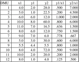
Table I- Outputs normalised by Input X1

DMU x1 y1 y2 y1/x1 y2/x1

1 4.0 2.0 28.0 .500 7.000 2 5.0 1.0 22.5 .200 4.500 3 6.0 6.0 12.0 1.000 2.000 4 10.0 8.0 60.0 .800 6.000 5 11.0 7.0 16.5 .636 1.500 6 8.0 6.0 12.0 .750 1.500 7 9.0 7.0 6.0 .778 .667 8 5.0 3.0 30.0 .600 6.000 9 5.5 4.4 5.5 .800 1.000 10 8.0 4.0 72.0 .500 9.000 11 10.0 2.0 20.0 .200 2.000 12 8.0 1.0 4.0 .125 .500

In this simple example, we can normalise the Outputs by the only Input and plot them in the plane. This is also equivalent to consider that we are dealing with a con-stant input of 1. This way we will be working in the plane defined by x=1 in the 3 dimensional one input two outputs space.

From Figure 1 it is easy to understand the reason for naming this technique Data Envelopment Analysis; in fact each DMU is analysed against the envelope of the most efficient units. For instance, the efficiency of DMU 8 is 0.857 (see Table II). This means that it could reduce its input to 85.7% of its current value reaching its target, Ci 8 (where Ci stands for Composite unit under minimi-sation of inputs), which is the same as for DMU 11 except that, for the latter, a reduction to 28.6% of X₁’s current level of inputs would be necessary for this DMU to become efficient, since its efficiency is only 0.286.

y1/x 0 1 2 3 4 5 6 7 8 9 0 0.1 0.2 0.3 0.4 0.5 0.6 0.7 0.8 0.9 1 12 11 10 9 8 7 6 5 4 3 2 1 Ci8;Ci11 C i 2 C i 9

Figure 1- Efficient frontier and radial projections for ineffi-cient units.

Although the results could be obtained graphically, we present in table II the results obtained by any stan-dard linear optimisation software.

Table II- Results for the multiplier problem

DMU _{µµµµ1111 νννν1111 νννν2222} Efficiency 1 0.250 0.179 0.018 0.857 2 0.200 0.000 0.022 0.500 3 0.167 0.152 0.008 1.000 4 0.100 0.091 0.005 1.000 5 0.091 0.083 0.004 0.647 6 0.125 0.114 0.006 0.750 7 0.111 0.111 0.000 0.778 8 0.200 0.143 0.014 0.857 9 0.182 0.182 0.000 0.800 10 0.125 0.089 0.009 1.000 11 0.100 0.071 0.007 0.286 12 0.125 0.114 0.006 0.136

IV. SUPEREFFICIENCY /DELETED DOMAIN EXTENSION

We arrive at the concept of Superefficiency by al-lowing the efficiency of the DMU being assessed to be greater than unity. This is achieved by removing the corresponding constraint from the set of J constraints in Expression (9). This is the reason why this technique is also known as deleted domain. The Superefficiency only affects units deemed as efficient, as the removed con-straint is not binding for the inefficient units, since their efficiency is, by definition, less than unity.

This extension to DEA was first published by Ander-sen and PeterAnder-sen [26] and its use is strongly recom-mended by the authors as a consequence of its simplicity and usefulness.

By using Superefficiency, it is possible to rank all units, even the efficient ones that by standard DEA techniques would all be rated as equal - their efficiency having reached the top value of 100%.

For the example presented in the previous section, the Superefficiency for the 3 efficient DMUs would be as presented in table III.

Table III- Superefficiency scores for the efficient units

Unit Superefficiency Unit 4 107.50% Unit 3 125.00% Unit 10 128.57%

Units 3 and 10 are efficient and robust, while any small increase in the Input or decrease in the Outputs of Unit 4 may make it inefficient.

An important additional benefit from this extension to the DEA model is that the set of weights is uniquely, determined for the efficient units in all practical applica-tions [21].

V. GRAPHICAL SOLUTION

The linear program defined by expressions (7) through (11) can be solved by the traditional graphical method if we have to deal with only 2 variables.

To reduce the problem from 3 to 2 variables, we will exploit the fact that we assume to be working under the constant returns to scale assumption and so we will scale all data to unity input level, so that our new data set will be the following one:

DMU Xn1 Yn1=y1/x1 Yn2=y2/x1

1 1 0.500 7.000 2 1 0.200 4.500 3 1 1.000 2.000 4 1 0.800 6.000 5 1 0.636 1.500 6 1 0.750 1.500 7 1 0.778 0.667 8 1 0.600 6.000 9 1 0.800 1.000 10 1 0.500 9.000 11 1 0.200 2.000 12 1 0.125 0.500

Table IV- Normalized data to unity input level

Since xn1=1 its multiplier µn1=1 and we have to solve

the linear program just for νn1 and νn2, we will illustrate

the results from the software EMS developed by Holger Scheel that uses an interior point solver.

Its results are presented in figure 2

Figure 2- Results obtained with the software EMS.

We can confirm the correctness of our results, namely that µn1=1 and that the values obtained for the efficiency

are equal to those previously presented in table II. It is worthy to note that DMUs F3, F7 and F9 place a minimal weight on Output2 while DMUs F2 and F10 choose to ignore Output1. This kind of problem is usu-ally solved by a technique known as weight restrictions in the sense of avoiding such a flexible set of weights and incorporating value judgments.

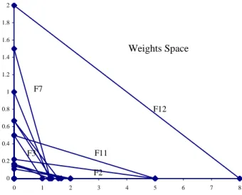
By solving graphically, we get the graph shown in figure 3 where we have 12 line segments, one for each constraint. The feasible region is the intersection of the twelve (lower) half planes containing the origin. It is

clear that inefficient units like F12 correspond to non-binding constraints and that the objective function is parallel to the respective DMU constraint.

0 0.2 0.4 0.6 0.8 1 1.2 1.4 1.6 1.8 2 0 1 2 3 4 5 6 7 8 Weights Space F12 F7 F11 F2 F3

Figure 3- Restrictions imposed by the 12 units in the Weights Space

For the sake of clarity, we will expand the previous picture just to the efficient units, in order to highlight the feasible region defined by the pentagon ABCD0 (in the clockwise direction). This feasible region is always the same for inefficient units for the efficient ones, it de-pends on the kind of model we are working with.

In the case of the traditional model the feasible re-gion is always identical, in the deleted domain case, also known as Superefficiency, the constraint related to the DMU being analysed is deleted, and even a non efficient Unit can pop-up in its reference set [21], this is the case of unit 10. In fact, its reference set is unit 1, since the feasible region on the weights space is EFCD0 (in the clockwise direction) and the objective function is paral-lel to the line segment 10, where it takes the unity value.

0 0 0 0 0 0 0 0 0 0 0 0 0 0.111... 0.1428... 1 1.25 0 0.05 0.1 0.15 0 0.5 1 1.5

10

3

4

A

B

C

D

1

Weights Space

E

F

Figure 4- Detail around the origin of the constraints imposed by the 12 units in the Weights Space

VI. WEIGHTS RESTRICTIONS

To avoid a given DMU “to choose” a rather unbal-anced set of weights (as is the case of units F2 and F10 which ignore Output 1 while F3, F7 and F9 ignore Out-put 2), it is current practice to place some restrictions on the weights or in the virtual inputs/outputs.

This is a usual way to incorporate judgment values and increase the discriminating potential of the model.

Restrictions on weights can be divided in two broad categories: Relative and absolute weights restrictions. As far as we know, only linear weights restrictions have been considered in the literature, thus we may present the weights restrictions in matrix form as follows:

BxµT +ByνT≤C

Where Bx∈ ℜcxm and By∈ ℜ cxn.

Dimension c refers to the number of constraints. If C ≠ 0 we refer to them as absolute weights restric-tions. The absolute weights restrictions are typically imposing a range for an individual weight. This ap-proach was developed by Dyson and Thanassoulis in 1988 [27] and generalized by Roll et al in 1991 [28]. Virtual weights restrictions introduced by Wong and Beasley in 1990 [29] belong to this category also. If C = 0 we speak about relative weights restrictions since if µ₀,ν₀ is a feasible solution so is k µ₀, k ν₀. The class of relative weights restrictions includes, among others, the assurance region models of Type I or II by Thompson et al in 1986 [30] and 1990 [31] respectively, as well as cone ratio DEA models from Charnes et al. in 1989 [32].

We can say that the most general approach is to re-strict the weights to belong to a closed set, being it a polytope or a polyhedral cone.

VII.WEIGHT ADJUSTMENT BY GOAL PROGRAMMING With standard DEA, it is common that many weights are null in the optimal solution. One way to avoid this situation is to place restrictions on the weights, but, in this case, weights typically used to cluster in the upper or lower limits. By including some non-linear but con-vex penalty in the objective function, penalizing devia-tions from a preference region in the weights space, it is possible to have a more uniform distribution of the weights.

This can be accomplished by the model, described by expressions 12 through 18 where G stands for Global objective function,

P

(d

r

)

is a penalizing function of the deviations dm and dn of the weights from the

exoge-nously imposed goals gm and gn.

The penalizing function will always be a convex one, for avoiding difficulties with local minima; it is worth recalling that since the feasible region is convex and the symmetric of the objective function is also convex, a local maximum is also a global maximum [33]. The definition of efficiency remains unchanged, so that this model just adjusts multipliers by a penalizing function

appended to the objective function scaled by a constant k. Max

(

)

1 ' ' '

v

y

k

P

d

N n njnj j

G

=

∑

−

×

r

= (12) s.t. dm=µmj’-gm m=1...M (13) dn=νnj’-gn n=1...N (14)

µ

mj mj m M

x

' ' =

∑

1 = 1 (15)

v y

nj nj n N ' =

∑

1 ≤

µ

mj mj m M

x

' =

∑

1 j=1...J (16) µmj’ ≥ε > 0 m=1...M (17) νnj’ ≥ε > 0 n=1...N (18) We will illustrate this technique with a simple exam-ple originating from the previous data set with 12 DMUs.

The preferred location for the weights is around the line 0.4ν_1j’=4ν_2j’. We are not interested in justifying this choice, neither other details like the value for the con-stant k, or the explicit kind of penalizing function, we also remind that our goal is just to exemplify a way to adjust weights in a smoother way than the usual hard restriction techniques do.

Therefore, the Global objective function will take the following form:

(

)

4

4

4

3

4

4

4

2

1

4

4

4

3

4

4

4

2

1

3

2

1

r Concave Strictly d P k Convex Strictly Penality Efficiency L N n njnj j is

y

v

G

→  × − = =

−

×

−

=

_∑

) ( ) ( 2 2 1 1 ' ' '

2

0

.

4

ν

4

ν

(19)

We will now illustrate the graphical solution for the evaluation of Unit 10 under the constant returns to scale assumption and deleted domain technique.

0 0.2 0.4 0.6 0.8 1 1.2 1.4 1.6 0 0.02 0.04 0.06 0.08 0.1 0.12 0.14 0.16 0.1-0.6 0.6-1.1 1.1-1.6 1.6-2.1 2.1-2.6

10

3

4

L=100.00%

G=.6

G=1.1

G=1.6

G=2.1

1

4

L=128.57%

In figure 5, the dotted lines correspond to constraints related to units 1, 3 and 4. The solid curves represent the isoquants of the Global objective function for G=0.6, 1.1, 1.6 and finally 2.1.

We can also see 3 solid straight lines:

1. The isoquant for L=100.00% that coincides with the constraint that was removed be-cause of the deleted domain technique. 2. The isoquant for L=114.06% as determined

by the exact quadratic programming solu-tion shown in table V.

3. The isoquant for L=128.57% that equals the score value from the Superefficiency tech-nique depicted in figure 2.

The optimal solution of the Superefficiency CCR model is the basic solution defined by the intersection of the constraint relative to unit 1 and µ₁≥ε > 0. It is inter-esting to note that an inefficient unit (DMU 1) is defin-ing the optimal solution for an efficient one, a fact first published in 1994 [21] by Santos and Themido.

The solution of the quadratic program can be ob-tained in a rough manner by the graphical method as exemplified in figure 5, or by the results shown in the line corresponding to DMU 10 in Table V.

Since the constraint relative to DMU 4 is the only binding one its Lagrange multiplier is the only one non-zero (λ4=1.000).

The optimum value for the objective function is G=1.070, which occurs at the point ν₁=0.51 ν₂=0.0982, deviating d= -0.188 from the preferred linear relation between weights, as a result we get the final value for efficiency of L=114.06%. This value is lower than the score obtained by the EMS software, since this new result has multipliers that are more desirable in the point of view of the incorporated weights preference structure, by the preferred linear relation between weights.

D

ν1 ν2 G d L λ3 λ4 λ10 1 .71 .0714 0.857 0.000 85.71% .000 0.24 .619 2 .68 .0732 0.465 -0.020 46.59% .000 0.00 .464 3 .92 .0434 0.934 0.196 101.15% .000 0.86 .000 4 .87 .0625 1.055 0.100 107.50% .245 0.00 .790 5 .83 .0547 0.589 0.117 61.60% .000 0.56 .000 6 .87 .0504 0.686 0.147 72.97% .000 0.64 .000 7 .90 .0455 0.671 0.182 73.76% .014 0.59 .000 8 .71 .0714 0.857 0.000 85.71% .000 0.57 .286 9 .90 .0459 0.707 0.179 77.04% .000 0.64 .000 10 .51 .0982 1.070 -0.188 114.06% .000 1.00 .000 11 .71 .0714 0.286 0.000 28.57% .000 0.19 .095 12 .73 .0692 0.125 0.016 12.60% .000 0.13 .000

Table V- Exact quadratic programming solutions

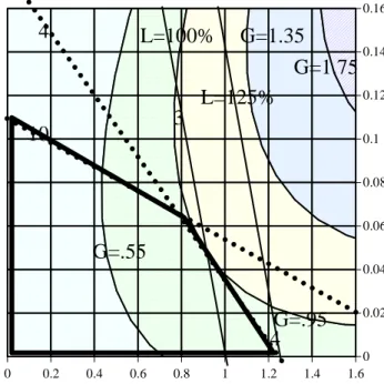
The objective function depends on the DMU being evaluated, in the previous picture DMU 10 was consid-ered; now we will show the graphical solution for DMU 3. 0 0.2 0.4 0.6 0.8 1 1.2 1.4 1.6 0 0.02 0.04 0.06 0.08 0.1 0.12 0.14 0.16

10

3

4

_L=100%

G=.55

G=.95

G=1.75

4

G=1.35

L=125%

Figure 6- Graphical solution for the evaluation of Unit 10

In figure 6 the dotted lines correspond to constraints related to units 10 and 4. The solid curves represent the isoquants of the Global objective function for G=0.55, 0.95, 1.35 and finally 1.75.

We can also see 2 solid straight lines:

1. The isoquant for L=100.00% that coincides with the constraint that was removed be-cause of the deleted domain technique, very close to the isoquant for L=101.15% as de-termined by the exact quadratic program-ming solution shown in table V.

2. The isoquant for L=125.00% that equals the score value from the Superefficiency tech-nique depicted in figure 2.

It is interesting to remark that the quadratic objective function isoquants have a different orientation from those depicted in figure 5, since the slope of the linear traditional linear objective functions were different too

Since the constraint relative to DMU 4 is the only binding one its Lagrange multiplier is the only one non-zero (λ4=0.857).

The optimum value for the objective function is G=0.934, which occurs at the point ν1=0.92 ν2=0.0434, deviating d= 0.196 from the preferred linear relation between weights, as a result we get the final value for efficiency of L=101.15%. Again, this value is lower than the score obtained by the EMS software, since this new result has multipliers that are more evenly distributed, around our goal: the line ν₂=0.1ν₁. The results without weight adjustment were an efficiency score of

L=125.00% but with a weight pattern neglecting output 2 (ν1=1.00 ν2=0).

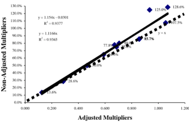
We can compare the score efficiencies obtained by the two models. The results are as depicted in figure 7

85.7% 50.0% 125.0% 107.5% 64.6% 75.0% 85.7% 80.0% 128.6% 28.6% 13.6% 77.8% y = 1.154x - 0.0301 R2 = 0.9377 y = 1.1166x R2 = 0.9365 y = x 0.0% 10.0% 20.0% 30.0% 40.0% 50.0% 60.0% 70.0% 80.0% 90.0% 100.0% 110.0% 120.0% 130.0% 0.000 0.200 0.400 0.600 0.800 1.000 1.200 Adjusted Multipliers N o n -A d ju st ed M u lt ip li er s

Figure 7- Comparison of efficiency scores

The dotted line is the line defined by y=x (restricted to the first orthant), to make it easy to see that all points are above or on that line, meaning that efficiency scores obtained with weight adjustment are not bigger than the ones obtained without adjustment. There are 3 DMUs (1, 8 and 11) which efficiency score remained un-changed, as a result of the fact that their optimal weights as shown in the EMS results in figure 2 were already complying with our later specification of staying on the line ν₂=0.1ν₁.

We can get the full detailed results for the other re-maining 10 DMUs by table V and locating their optimal weights in figures 5 or 6.

It is now worth noting that DMUs 1 and 8 have ex-actly the same score and the same optimal weights, since the relation ν₂=0.1ν₁ implies an intrinsic marginal rate of substitution of y1 by y2 of ν1/ν2=10 which is exactly

the case for their outputs. The fact that two of its La-grange multipliers are the only non-zero ones (λ4and λ10) means that its optimal weights are in the intersection of the two straight lines relative to the bind-ing restrictions of DMUs 4 and 10.

Now we will introduce a last graphical example of the solution of the CCR Model of the data set presented in figure 8 where we consider one input X=1 and two outputs YC1 and YC2 whose name comes from the

ap-pearance of the 99 points in circular layers in the first orthant.

It is time to explain that the solver for non-linear programs we are using is limited to 100 constraints and this is the reason why we do not solve bigger instances.

In the figure 9, we also present the results of the EMS software under deleted domain and Constant Re-turns to Scale assumption.

0 0.2 0.4 0.6 0.8 1 0 0.2 0.4 0.6 0.8 1 YC1 Y C 2 D1 D34 D99 D33 D66 D67 L=100.13% L=80.00% L=90.00 %

Figure 8- Data for an example of absolute weights adjust-ment

This time the deviation at the penalizing function was defined as the squared distance from the average of the standard DEA weights normalized by its standard devia-tion. 2 2 1 2 1 1 2 1 ) (                −    +                −    =

σ

µ

ν

σ

µ

ν

ν ν ν ν d P r (20)

The meanings of the parameters in expression 20 are as follows:

νj is the unknown weight for YCj.

µνj is the average of the weight νj determined solving the

standard DEA CCR model under deleted domain.

σνj is the standard deviation of the weight νj found

solv-ing the standard DEA CCR model under deleted do-main.

The efficiency scores for this absolute adjustment are shown in figure 9, where the highest efficiency score of 100.13% is attained by a single DMU. In fact, the 17th DMU has the same weights than those obtained by the standard minimization of inputs DEA CCR model under deleted domain

0.6800 0.7800 0.8800 0.9800

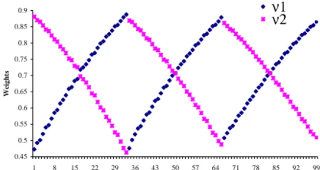
In figure 10, we present the resulting weights that in-stead of clustering at the upper and lower limits of its absolute weights restrictions, as happens with traditional weights restriction techniques, now they spread around the central previously defined value νννν=(0.6;0.6). We do not know of any other public work that can ac-complish such versatility as this technique.

This method can be further enhanced by the introduction of special types of penalty functions like Tchebychev polynomials, or maximally flat polynomials.

0.45 0.5 0.55 0.6 0.65 0.7 0.75 0.8 0.85 0.9 1 8 15 22 29 36 43 50 57 64 71 78 85 92 99 W ei g h ts ν1 ν2

Figure 10- Optimal weights distributing around 0.6

VIII. APPLICATION TO A CASE WITH ARTIFICIALLY GENERATED DATA

Finally we will apply this multiplier adjustment tech-nique to a case with two outputs and four inputs, with simulated data.

Data generating process

When generating the data for the experiments re-ported in this section we considered two factors: produc-tion technology, and inefficiency distribuproduc-tion

Production technology

We considered a two outputs and four inputs produc-tion technology. This was obtained through the genera-tion of a single aggregate output incorporating an ineffi-ciency stochastic factor and later split in two outputs as suggested in 1997 by Durchholz and Barr [34].

The single Cobb-Douglas aggregate output and four inputs production technology is specified in terms of its efficient production function z = f (x1, x2 x3, x4), where z

represents the maximum aggregate output that can be produced from the levels x1, x2, x3 and x4 of the four

inputs. Specifically, we used the following shifted Cobb-Douglas production function:

i i i i

x

z

_a

(

α

)

β 4 1 0

−

=

∏

= (21)

ao is a constant scale factor.

αi is the shift from the origin for input i.

βi is the factor elasticity for input i.

z is the single Cobb-Douglas aggregate output If ∑βi = 1, then only constant returns to scale exist in the production process. For ∑βi < 1, decreasing returns to scale are present, while ∑βi > 1 indicates increasing returns to scale.

In DEA, increasing returns to scale are not used be-cause the function results in only a few DEA efficient points, since for higher levels of input than those defined by the Most Productive Scale Size the Production Pos-sibilities Set is the polyhedral cone from the CCR model. Although this does not pose a problem, it does not represent realistic data.

We made ao= 1, α1= α2= α3= α4= 5, the input levels

x1, x2, x3 and x4 were generated randomly from four

independent uniform probability distributions over the interval [10, 20], and the coefficients β1, β2, β3, and β4

were randomly generated from independent uniform probability distributions over the interval [0.20, 0.25]. Since the sum of β1, β2, β3, and β4 is less than one, the

production function in expression 21 satisfies the DEA-BCC models assumption of a strictly concave produc-tion funcproduc-tion, while the shifts α1= α2= α3= α4= 5 > 0

allow both increasing and decreasing returns to scale to prevail.

Inefficiency distribution

We generated the logarithm of the inefficiency, u=ln θ from a half-normal distribution | N (

0

;

σ

2

u ) |,

where the parameter

σ

2

u itself is drawn from a uniform

distribution on the interval [0, 0.1989]. The range of values for the distribution of

σ

2

u is chosen in such a

way that the mean efficiency given by E(h=1/θ)=

e

u π

σ

2/ − is between 0.7 and 1.0. Simulated observations

We first generated random values for βi between 0.2 and 0.25, and a value

σ

2

u between 0 and 0.1989. Next,

we simulated 90 observations of the four inputs x1

through x4between 10 and 20. Those values were then

substituted into the efficient production function speci-fied in expression 21 to obtain the corresponding values zj = f (xij) for the efficient output quantity. Then, we

randomly generated the logarithm of actual inefficiency values uk=lnθk, for each one of the 90 observations from

the half-normal distribution | N (

0

;

σ

2

u ) |.

Finally, we obtained the values for observed aggre-gated output quantities yj as: yj = f(xij)/exp(uj) and the

true efficiency value hk=1/exp(uk).

Once the single aggregate output level y was

calculated, the two individual output levels were

determined by assigning each individual output as

a percentage of the aggregate. The percentages for

each individual output were drawn from normal

distributions with predetermined means and

stan-dard deviations. The means of the normal

distribu-tions were chosen so that the percentages sum up

to one. In our specific case, we chose each normal

distribution to have a mean of 0.5 and a standard

deviation of 0.1.

The results from the unbounded model solved

by the EMS software are summarized in table VI:

Eff. µ1µ1µ1µ1 µ2µ2µ2 µ3µ2 µ3 µ4µ3µ3 µ4µ4µ4 ν1ν1ν1 ν2ν1 ν2ν2ν2 Average 84% .03 .01 .01 .02 .09 .18 Standard Dev. 19% .03 .02 .02 .03 .08 .09 Coef. of Var. .222 .99 1.53 1.98 1.31 .87 .51 Maximum 127% .10 .10 .10 .10 .28 .32 Percentile 75% 97% .06 .02 .01 .04 .14 .24 Percentile 50% 85% .03 .00 .00 .01 .06 .20 Percentile 25% 70% .00 .00 .00 .00 .03 .15 Percentile 4% 55% .00 .00 .00 .00 .00 .00 Minimum 44% .00 .00 .00 .00 .00 .00 Table VI- Statistical descriptors of the results for the EMS

software (CCR model, minimization of inputs).

Eff. µ1µ1µ1µ1 µ2µ2µ2µ2 µ3µ3 µ4µ3µ3 µ4µ4µ4 ν1ν1ν1 ν2ν1 ν2ν2ν2 Average 74% .035 .012 .007 .018 .074 .176 StandardDev. 16% .014 .005 .003 .011 .051 .064 Coef.of Var. .221 .403 .421 .393 .633 .692 .367 Maximum 123% .066 .024 .014 .042 .247 .276 Percentile 75%90% .045 .015 .008 .027 .098 .218 Percentile 50%81% .034 .011 .007 .017 .052 .192 Percentile 25%65% .023 .009 .005 .008 .042 .155 Percentile 4% 48% .015 .003 .002 .000 .027 .035 Minimum 42% .012 .002 .001 .000 .002 .000 Table VII- Statistical descriptors of the results for our new

model (CCR model, minimization of inputs).

From the comparison between table VI and table VII we notice that:

The Statistical descriptors of the efficiency scores in our model are always lower. This was expected since penalties may occur and our global objective function never exceeds the traditional linear one.

The Average efficiency score in the classical CCR model is 84%, as was expected from the assumptions about the Half Normal distribution of the inefficiency.

The standard deviation of any multiplier is lower than the corresponding one in the non-adjusted case (this could originate from the decrease in the average values; that lead us also to compute the coefficient of variation, confirming that, even in relative terms, the weights are not as spread as in the original model.

The same conclusion also holds to any other measure (Maximum and percentiles).

Only when it comes to the minima of µ4 and ν2, we

have a tie, but even in this case it is sufficient to take into account the values for the lower percentiles. In fact,

µ4 vanishes 35 times in the traditional linear model, in

opposition to just 5 zeros in our model.

In the case of ν2, the proportion is similar: there are

only two null weights in the adjusted case against 13 on the classic one.

It should be noted that it would be easy to avoid the occurrence of null weights simply by increasing the steepness of the convex penalty function, although this was not our choice, since it could lead to a point that no DMU at all would reach the 100% efficiency score

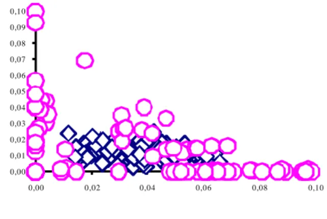
In an effort to show our results in the 6 dimensional weights space, we illustrate in figures 11 through 13 its projections on the bidimensional spaces. In these fig-ures, the circles represent the weights for the traditional model and the diamonds correspond to those obtained by our model. 0,00 0,01 0,02 0,03 0,04 0,05 0,06 0,07 0,08 0,09 0,10 0,00 0,02 0,04 0,06 0,08 0,10

Figure 11- Distribution of µ1 (in the vertical axis) and µ2 (in the horizontal axis)

In figure 11, we can confirm that µ1 and µ2 cluster

over the both axes, if we do not apply our adjustments on multipliers. In fact, µ1 vanishes 31 times and about µ2

this happens 43 times.

0,00 0,01 0,02 0,03 0,04 0,05 0,06 0,07 0,08 0,09 0,10 0,00 0,02 0,04 0,06 0,08 0,10

Figure 12- Distribution of µ3 (in the vertical axis) and µ4 (in the horizontal axis)

The considerations made about figure 11 also apply to figure 12 but here µ3 has 38 zeros and µ4 has 35. As a

result of applying our technique only µ4 kept some

ze-ros, but nevertheless its number dropped to 5. It is worth mentioning that not only did we avoid the occurrence of zeros, but we also reduced its maximal values.

0, 00 0, 05 0, 10 0, 15 0, 20 0, 25 0, 30 0, 35 0,00 0, 05 0, 10 0,15 0, 20 0, 25 0,30

Figure 13- Distribution of ν1 (in the vertical axis) and ν2 (in the horizontal axis)

In figure 13, since we are dealing with only two out-puts, the benefits of our method are not as evident as in the input case. Regardless of that, from the initial 13 DMUs that presented a null weight in output Y2, this number decreased to only 2 of the initial 13, namely DMU 41 and DMU 61.

If we had had more outputs, our technique would have been more useful, in the sense that the number of zeros to reduce would have been greater.

We tried to make this representation in several graphic ways, but this one seemed to us to be the best. We also investigated if the use of a data reduction technique like factor analysis, could be of some help, but the correla-tion matrix did not allow for an easy alternate represen-tation of the data.

y = 1.03 22 x + 0.04 R2 = 0 .9 244 y = 1.0 81 1x R2 = 0.92 22 30 % 40 % 50 % 60 % 70 % 80 % 90 % 100 % 110 % 120 % 130 % 30% 40% 50 % 60% 70% 80% 90 % 100% 1 10% 120% 130% 6 1

Figure 14- Representation of the Score obtained by the EMS software and our efficiency values

In figure 14, we plot the results for both the score ob-tained by the EMS software and our efficiency values. We notice that our values never exceed those from the CCR model and that in some cases there is a substantial reduction on the original value as is the case by instance

of DMU 61 whose efficiency value dropped from an original value of 124% to 102%.

Despite this fact, it is important to remark the existence of a strong correlation between the two variables, and so we made a linear regression on it.

Although the model with a constant leads to a higher determination coefficient of 0.9244, this constant has a p value of 0.11, and therefore, it is not significant. Thus we conclude that the EMS Scores exceed in 8% those from our model.

IX. CONCLUSIONS

This paper introduces a new way of adjusting weights, a matter that has already deserved many publi-cations in the Data Envelopment Analysis field. This new method adds greater flexibility to the weight restric-tions techniques. It is not our concern to present the potentialities or the details of weight restrictions. This matter is already extensively covered in the existing literature, namely on how to set up the specific values for the restrictions.

Since we are dealing with a non-linear concave ob-jective function, we have the possibility to locate the optimal set of weights in a continuous way in contrast to the linear case where optimality always occurs at a ver-tex of the feasible solution set.

We used the simplest convex penalty function for the sake of clarity, but other convex functions like maxi-mally flat polynomials or Tchebychev polynomials could also be used.

Even the convexity restriction can be dropped leading to more complicated programs, that can be used for instance in discriminating analysis.

REFERENCES

[1] Milind Sathye (2003), “Efficiency of banks in a developing economy: The case of India”.

Euro-pean Journal of Operational Research, 148, (3)

662-671

[2] Thanassoulis, E. and P. Dunstan, (1994), “Guiding schools to improved performance using data en-velopment analysis: An illustration with data from a local education authority”, Journal of the

Opera-tional Research Society, 45, (11), 1247-1262.

[3] Thanassoulis, E., (1993), “Comparison of regres-sion analysis and data envelopment analysis as al-ternative methods for performance assessments”,

Journal of the Operational Research Society, 44,

(11), 1129-44.

[4] Boussofiane, A., R. G. Dyson, Thanassoulis, E., (1991), “Applied data envelopment analysis”,

European Journal of Operational Research, 52,

(1), 1-15.

[5] Charnes, A., Cooper, W. W., Rhodes, E., (1978), “Measuring the efficiency of decision making

units”, European Journal of Operations Research, 2, (6), 429-44.

[6] Farrell, M. J., (1957), “The measurement of pro-ductive efficiency”, Journal of Royal Statistical

Society A, 120, 253-281.

[7] Chang, K.-P. and Y.-Y. Guh, (1991), “Linear production functions and the data envelopment analysis”, European Journal of Operational

Re-search, 52, (2), 215-23

[8] Rhodes, E., (1978), “Data envelopment analysis and related approaches for measuring the effi-ciency of decision-making units with an applica-tion to program follow through in U.S. educaapplica-tion”, unpublished doctoral thesis, School of Urban and Public Affairs, Carnegie - Mellon University. [9] Nunamaker, T. R. and A. Y. Lewin, (1983),

“Measuring routine nursing service efficiency: A comparison of cost per patient day and data envel-opment analysis models”, Health Services

Re-search, 18, (2 (Part 1)), 183-208.

[10] Thanassoulis, E., A. Boussofiane, R. G. Dyson,(1995), “Exploring output quality targets in the provision of prenatal care in England using data envelopment analysis”, European Journal of

Operational Research, 80, (3), 588-607.

[11] Ganley, J. A., Cubbin, J. S., (1992), Public Sector

Efficiency Measurement - Applications of Data Envelopment Analysis, North - Holland, 57-80.

[12] Lewin, A. Y. and R. C. Morey, Cook, T.J., (1982), “Evaluating the Administrative Efficiency of Courts”, Omega, 10 ,(4), 401-11.

[13] Chu, X. and G. J. Fielding, (1992), “Measuring transit performance using data envelopment analysis”,

Transportation Research Part A (Policy and

Prac-tice), 26A, (3), 223-30.

[14] Thompson, R. G., Dharmapala, P. S., Thrall, R., (1995), “Sensitivity analysis of efficiency measures with applications to Kansas farming and Illinois coal mining”, Data Envelopment Analysis: Theory,

Meth-odology and Applications,. A. Charnes, W. W.

Coo-per, A. Lewin and L. M. Seiford. Boston, Kluwer Academic Publishers, 89-94.

[15] Schefczyk, M., (1993), “Operational performance of airlines: an extension of traditional measure-ment paradigms”, Strategic Managemeasure-ment Journal, 14, 301-317.

[16] Vassiloglou, M. and D. Giokas, (1990), “A study of the relative efficiency of bank branches: an ap-plication of data envelopment analysis”, Journal of

the Operational Research Society , 41, ( 7), 591-7.

[17] Bessent, A., Bessent, W., Kennington, J., e Regan, B., (1982), “An application of Mathematical Pro-gramming to assess productivity in the Houston independent school district”, Management

Sci-ence, Vol. 28, No. 12, 1355-67.

[18] Charnes, A., Cooper, W.W., Rhodes, E., (1981), “Evaluating program and managerial efficiency: an application of Data Envelopment Analysis to Pro-gram Follow Through”, Management Science, 27, (6), 668-97.

[19] Charnes, A., Cooper, W.W., e Rhodes, E., (1978), “Measuring the efficiency of decision making units”, European Journal of Operational

Re-search, 2, (6), 429-44.

[20] Castro, R., (1993), “O método DEA - Aplicação à avaliação da eficiência comparativa das escolas secundárias do distrito do Porto”, unpublished Msc. thesis, Faculdade de Economia, University of Oporto.

[21] Santos, J., (1994), “Ordenação de unidades eficientes por técnicas de data envelopment analysis”, unpublished Msc. thesis, Instituto Superior Técnico, Technical University of Lisbon.

[22] Beasley, J.E., (1990), “Comparing university de-partments”, Omega, 18, 171-83.

[23] Charnes, A., Cooper, W.W., Rhodes, E., (1978), “Measuring the efficiency of decision making units”, European Journal of Operational

Re-search, 2, (6), 429-44.

[24] Charnes, A., Cooper, W. W., Rhodes, E., (1979), “Short communication: measuring the efficiency of de-cision making units”, European Journal of Operational

Research, 3, (4), 339.

[25] Charnes, A., Cooper, W.W., (1962), “Program-ming with linear fractional functionals”, Naval

Re-search Logistics Quarterly, 9, 181-185.

[26] Andersen, P., Petersen, N.C., (1993), “A proce-dure for ranking efficient units in data envelop-ment analysis”, Manageenvelop-ment Science, 39 ,(10), 1261-4.

[27] Dyson, R. G. and E. Thanassoulis (1988). "Reduc-ing weight flexibility in data envelopment analy-sis." Journal of the Operational Research Society 39( 6): 563-76

[28] Roll, Y., W. Cook, et al. (1991). "Controlling factor weights in data envelopment analysis." IIE

Transactions 23( 1): 2-9.

[29] Wong, Y.-H. B. and J. E. Beasley (1990). "Re-stricting weight flexibility in data envelopment analysis." Journal of the Operational Research

Society 41( 9): 829-35.

[30] Thompson, R. G., F. D. Singleton, Jr., et al. (1986). "Comparative site evaluations for locating a high-energy physics lab in Texas." Interfaces 16( 6): 35-49.

[31] Thompson, R. G., L. N. Langemeier, et al. (1990). "The role of multiplier bounds in efficiency analy-sis with application to Kansas farming." Journal of

[32] Charnes, A., Cooper, W., Wei, Q., and Huang, Z. (1989), “Cone Ratio Data Envelopment Analysis and Multi-Objective Programming”, International

Journal of Systems Science 20, 1099-1118.

[33] Frederick S. Hillier, Gerald J. Lieberman,

Intro-duction to Operations Research, Mc Graw Hill,

1990.

[34] Durchholz, M. and R. Barr (1997). "Parallel and hierarchical decomposition approaches for solving large-scale data envelopment analysis models."