CERN-EP/2017-035 2017/03/21
CMS-B2G-16-013
Search for a heavy resonance decaying to a top quark and a
vector-like top quark at
√
s
=
13 TeV
The CMS Collaboration
∗Abstract
A search is presented for massive spin-1 Z0 resonances decaying to a top quark and a heavy vector-like top quark partner T. The search is based on a 2.6 fb−1 sample of proton-proton collisions at 13 TeV collected with the CMS detector at the LHC. The analysis is optimized for final states in which the T quark decays to a W boson and a bottom quark. The focus is on all-jet final states in which both the W boson and the top quark decay into quarks that evolve into jets. The decay products of the top quark and of the W boson are assumed to be highly Lorentz-boosted and cannot be reconstructed as separate jets, but are instead reconstructed as merged, wide jets. Techniques for the identification of jet substructure and jet flavour are used to distinguish signal from background events. Several models for Z0 bosons decaying to T quarks are excluded at 95% confidence level, with upper limits on the cross section ranging from 0.13 to 10 pb, depending on the chosen hypotheses. This is the first search for a neutral spin-1 heavy resonance decaying to a top quark and a vector-like T quark in the all-hadronic final state.
Submitted to the Journal of High Energy Physics
c
2017 CERN for the benefit of the CMS Collaboration. CC-BY-3.0 license
∗See Appendix A for the list of collaboration members
arXiv:1703.06352v1 [hep-ex] 18 Mar 2017
1
Introduction
Many theoretical models of physics beyond the standard model (SM) predict the existence of heavy bosonic resonances [1–9]. Such resonances include Z0gauge bosons [10–12] and Kaluza– Klein excitations of a gluon in Randall–Sundrum models [13, 14]. In many cases the couplings of these resonances to third-generation SM quarks are enhanced, leading to decay channels containing top quarks.
The CMS and ATLAS Collaborations at the CERN LHC have performed several searches for heavy resonances decaying to top quark-antiquark pairs (tt) [15–21], placing very stringent limits on their production cross sections. However, in models with a heavy gluon [22, 23], a composite Higgs boson [24], or extra spatial dimensions [22, 25], an additional fermionic sector may be present in the form of a nonchiral (or vector-like) fourth generation of quarks. Topologies in which the Z0 boson decays into vector-like quarks have not yet been investigated experimentally. This search focuses on the kinematic range in which Z0 boson decays to tT dominate over those to TT, where T is a vector-like heavy quark with a charge of two thirds. Vector-like quarks are fermions whose left- and right-handed components transform in the same way under the electroweak symmetry group of the SM. Consequently, their masses can be generated through direct mass terms in the Lagrangian, rather than via Yukawa couplings. This feature makes theories that include a heavy vector-like quark sector compatible with current Higgs boson measurements [26].
We present results of the first search for neutral spin-1 heavy resonances decaying to a top quark and a vector-like T quark, in all-jet final states. The search is optimized for the T →bW
decay mode, but also considers T → tH and T → TZ decays. The analysis is based on data
from proton-proton collisions collected by the CMS experiment at a centre-of-mass energy of 13 TeV, corresponding to a total integrated luminosity of 2.6 fb−1.
The results of the analysis are compared with the predictions of two theoretical models. The first model [22] is an effective theory with one warped extra dimension that considers only the lowest-energy spin-1 and spin-1/2 resonances to describe the decays of the lightest Kaluza– Klein excitation of the gluon, G∗, to one SM particle and one heavy fermion. We consider the specific case where the G∗resonance decays to a top quark and a heavy top quark partner T. The model assumes branching fractions (B) to be 50/25/25% for T quark decay to the bW/tH/tZ channels. Benchmark values of tan θ3 =0.44, sin φtR =0.6, and Y∗ = 3 are used for the model
parameters. The definitions of the parameters, the choice of their values, and their impact on the cross section are explained in [22].
The second model [24] is a minimal composite effective theory of the Higgs boson based on the coset SO(5)/SO(4), describing the phenomenology of heavy vector resonances, with particular focus on their interactions with top quark partners. The results of the analysis are compared with the cross section for the production of a neutral spin-1 resonance ρ0L decaying to a top quark and a heavy top quark partner T. The model assumes T branching fractions to tH/tZ channels of 50/50%. The following are benchmark values of the model parameters: yL =c3 =
c2 = 1, and gρL =3. The model parameters and the choice of benchmark values are described
in [24]. This model is used to simulate signal samples.
The G∗ and the ρ0L resonances are candidates for the Z0 of this search and are both produced through quark-antiquark pair interactions at the LHC. The kinematic distributions of the decay modes considered are comparable between the two models. Hypothetical top quark flavour-changing neutral currents generated in the interaction between the top quark, Z0 boson, and T quark are estimated to be below the reach of current measurements [27] because of the large
2 2 The CMS detector
suppression generated by off-shell effects of the Z0 boson and the T quark. The leading order Feynman diagram for the production of the Z0boson and the decay chain under consideration is depicted in Fig. 1.
Z
′¯
t
T
W, H, Z
b, t
¯
q
q
Figure 1: The leading order Feynman diagram showing the production mode of the Z0 boson
and its decay chain.
Because of the large difference in mass between the W boson and the T quark, the W boson receives a large Lorentz boost, such that its decay products appear as merged jets (in a highly-boosted topology). Jet substructure algorithms are employed to reconstruct and identify the W boson originating from the decay of the T quark. If the mass difference between the Z0 boson and the T quark is much larger than the mass of the top quark, the top quark from the decay of the Z0boson also receives a large transverse momentum (pT), in which case jet-substructure
techniques can also be used to identify and reconstruct the all-jets decay of the top quark. The dominant background is from SM events and is comprised of jets produced through the strong interaction, i.e. quantum chromodynamics (QCD) multijet events, followed by events from tt pair production and from single top quark production. The contribution of the latter processes is estimated from simulation, while the multijet QCD background is estimated from data using signal-depleted control regions.
This paper is organized as follows: Section 2 gives a description of the CMS detector and the reconstruction of events. Section 3 describes the data and the simulated samples used in the analysis. An overview of the jet-substructure algorithms and the details of the selection for the analysis are given in Section 4. Estimation of SM background processes is discussed in Section 5, while Section 6 describes the systematic uncertainties. The results of the analysis and a summary are given in Sections 7 and 8, respectively.
2
The CMS detector
The central feature of the CMS apparatus is a superconducting solenoid of 6 m internal diame-ter, providing a magnetic field of 3.8 T. Within the solenoid volume are a silicon pixel and strip tracker, a lead tungstate crystal electromagnetic calorimeter (ECAL), and a brass and scintilla-tor hadron calorimeter (HCAL), each composed of a barrel and two endcap sections. Forward calorimeters extend the pseudorapidity (η) coverage provided by the barrel and endcap detec-tors. Muons are measured in gas-ionization detectors embedded in the steel flux-return yoke outside the solenoid.
A particle-flow event algorithm [28, 29] reconstructs and identifies each individual particle with an optimized combination of information from the various elements of the CMS detector.
The energy of photons is directly obtained from the ECAL measurement, corrected for zero-suppression effects. The energy of electrons is determined from a combination of the electron momentum at the primary interaction vertex as determined by the tracker, the energy of the corresponding ECAL cluster, and the energy sum of all bremsstrahlung photons spatially com-patible with originating from the electron track. The energy of muons is obtained from the curvature of the corresponding track. The energy of charged hadrons is determined from a combination of their momentum measured in the tracker and the matching ECAL and HCAL energy deposits, corrected for zero-suppression effects and for the response function of the calorimeters to hadronic showers. Finally, the energy of neutral hadrons is obtained from the corresponding corrected sum of ECAL and HCAL energies. Primary vertices are reconstructed using a deterministic annealing filter algorithm [30]. The vertex with the largest sum of the squares of the associated track pT values is taken to be the primary event vertex. A more
de-tailed description of the CMS detector, together with a definition of the coordinate system used and the relevant kinematic variables, can be found in Ref. [31].
3
Data and simulation samples
The events are selected with an online trigger that required the scalar pT sum of the jets (HT)
to be larger than 800 GeV. The offline HT is required to be larger than 850 GeV. After this
selection, the trigger is more than 97% efficient in selecting those events that would pass the analysis selection. The trigger and offline HTselections do not significantly impact the overall
signal efficiency because the masses of the spin-1 resonances considered in this analysis are at least 1.5 TeV.
The signal processes are simulated using MADGRAPHv5.2.2.2 [32]. Neutral spin-1 resonances (Z0boson) decaying exclusively to a top quark and an up-type heavy vector-like quark (T) are generated. Data samples are produced for three values of mass of the Z0boson and a width of 1% the mass. For the T quark samples the width of the quark is fixed to 1 MeV. The values of the width are chosen to be much smaller than the detector resolution. The T quark is generated with left-handed chirality. The impact of the chirality of the T quark on the analysis is assessed on a single signal configuration and is found to be insignificant, and for this reason the right-handed chirality case is not explicitly considered.
The simulation of the signal event production is based on a simplified low-energy effective theory describing the phenomenology of heavy vector resonances in the minimal composite Higgs model [24]. Signal samples are generated for three decay modes of the T quark: T→bW, tH, and tZ. Several mass hypotheses for the Z0 (T) resonance are considered ranging from 1.5 to 2.5 (0.7 to 1.5) TeV. The combination of the Z0 and T masses is chosen such that the mass of the T quark is roughly 1/2, 2/3, or 5/6 of the Z0 boson mass. With this choice of masses, the Z0 decay into a T quark-antiquark pair is kinematically suppressed. For some of the samples generated, the top quark from the decay of the Z0boson receives a small pTand its decay does
not result in a boosted topology.
The decay of heavy resonances in signal events is processed with MADSPIN[33] to correctly treat the spin correlations in the decay chain. The matrix element calculations for signal pro-cesses include one extra parton at most emitted at tree level. To model fragmentation and parton showering, thePYTHIA8.2 [34] tune CUETP8M1 [35] is used, and the MLM scheme [36] is used to match parton emission in the matrix element with the parton shower. Differential jet rates are checked for smoothness to ensure that the matching scale is chosen correctly.
4 4 Event reconstruction and selection
POWHEG V2 [37–41]. The tt event sample is normalized to the next-to-next-to-leading order
(NNLO) cross section of σtt = 831.76 pb [42]. Background events from single top quark pro-duction in the tW channel are also generated withPOWHEG V2 and are normalized to a cross section of 71.7 pb [43]. Single top quark production in the s and t channels without an associ-ated W boson is generassoci-ated with MADGRAPHv5.2.2.2 [32] and the cross sections are normalized to 10.32 and 216.99 pb, respectively [44, 45]. All samples are interfaced toPYTHIA8.2 for frag-mentation and parton showering. The multijet QCD production is estimated from data. Simu-lated multijet QCD events are used only to validate the method of background estimation and are generated with PYTHIA8.2, binned in HT to increase the event sample in the high-energy
region.
All events were generated with the NNPDF 3.0 parton distribution functions (PDFs) [46]. All simulated event samples include the simulation of additional inelastic proton-proton interac-tions within the same or adjacent bunch crossings (pileup). The detector response is simulated with the GEANT4 package [47, 48]. Simulated events are processed through the same software chain as used for collision data and are reweighted to match the observed distribution of the number of pileup interactions in data.
4
Event reconstruction and selection
For each event, hadronic jets are clustered from the reconstructed particles with the infrared and collinear safe anti-kT algorithm [49], using the FASTJET3.0 software package [50? ] with
the distance parameters R= 0.4 (AK4 jets) and 0.8 (AK8 jets). The two types of jets are recon-structed independently. Charged hadrons not associated with the primary vertex of the inter-action are not considered when clustering. Corrections based on the jet area [51] are applied to remove the energy contribution of neutral hadrons arising from pileup collisions. Further corrections are used to account for the nonlinear calorimeter response as a function of η and pT [52], derived from simulation and from data-to-simulation correction factors. Spurious jets
due to detector noise effects are removed by requiring that neutral particles contribute less than 99% of the electromagnetic and hadronic energy in a jet. Only jets with|η| <2.4 are considered;
no requirements on lepton or imbalance in transverse momentum are applied.
This analysis considers signal events characterized by a three-jet topology. One of the jets corresponds to the boosted top quark from the decay of the Z0 boson, the second originates from the W boson of the T quark decay, and the third is from the b quark emitted in the T quark decay. These selection criteria are optimized for the decay of the T quark to bW, but the analysis is sensitive to the other decay modes of the T quark as well. To identify t jets, the jets associated with top quarks, the “CMS top tagger v2” [53] algorithm is used. In this algorithm, the constituents of the AK8 jets are reclustered using the Cambridge–Aachen algorithm [54, 55]. The modified mass-drop tagger algorithm [56], also known as the “soft drop” algorithm with angular exponent β = 0, soft threshold zcut < 0.1, and characteristic radius R0 = 0.8 [57], is
used to remove soft, wide-angle radiation from the jet. This algorithm identifies two subjets within the AK8 jet corresponding to the b jet and the decay of the W boson. Additionally, the “N-subjettiness” variables τN [58, 59] are used. These variables, calculated using all the
particle-flow constituents of the AK8 jet, quantify the degree to which a jet can be regarded as composed of N subjets.
For the identification of top quark candidates, the soft-drop mass, mSD, is required to satisfy
110< mSD<210 GeV and the N-subjettiness variable is required to satisfy τ3/τ2<0.86. These
selections correspond to a misidentification rate of 10% for multijet QCD, and an efficiency greater than 70%. To ensure that the decays of the top quark are merged in a single jet, AK8 jets
are required to have pT > 400 GeV. Jets satisfying the aforementioned momentum, mass, and
N-subjettiness selections are referred to as “t-tagged”.
For the identification of W jets, the same jet reclustering procedure as in the t tagging algorithm is chosen. Additionally, jets are required to fulfill 70 < mSD < 100 GeV, τ2/τ1 < 0.6, and
pT > 200 GeV. These criteria correspond to a misidentification rate of approximately 5% for
multijet QCD, and an efficiency of approximately 60% for genuine W bosons not coming from the decay of a top quark. Jets satisfying these requirements are referred to as “W-tagged”. The Combined Secondary Vertex v2 (CSVv2) algorithm [60, 61] is used to identify AK4 jets originating from b quarks (b tagging). The ‘medium’ working point of the algorithm is used, which provides an efficiency of approximately 70% for the identification of genuine b quark jets while rejecting 99% of light-flavour jets. The ‘loose’ working point of the algorithm is used for the background estimation, providing an efficiency of approximately 85% and a light-flavour rejection rate of 90%. Additionally, t-tagged jets with a b-tagged subjet [20, 61] are used to improve the discrimination power against background processes. The CSVv2 algorithm with the ‘medium’ working point is used for subjet b tagging.
The events are required to have at least one b-tagged AK4 jet [60], with pT > 100 GeV and
|η| < 2.4. To avoid possible overlaps, the AK4 jet is required to have an angular separation,
∆R, of at least 0.8 with respect to the t-tagged jet and the W-tagged jet. The angular separation variable ∆R is defined as√(∆φ)2+ (∆η)2, where φ is the azimuthal angle. Among the b jets satisfying these requirements, the one with the highest pT is selected. The T quark candidate
four-momentum is defined as the sum of the 4-vectors of the selected b jet and the W-tagged jet. Only events with a T quark candidate mass mT >500 GeV are considered. This selection
crite-rion helps to reject the tt background. The reconstructed Z0 boson candidate four-momentum is defined as the sum of the 4-vectors of the T quark candidate and the selected t-tagged jet. The invariant mass of the Z0 boson candidate mZ0 is used as the main discriminating observable in
the analysis.
Events are grouped into two separate categories according to the presence or absence of a b-tagged subjet in the t-b-tagged jet. Events containing a b-b-tagged subjet are placed in the “SR 2 b tag category” as they contain one b-tagged AK4 jet together with a b-tagged subjet associated with the t-tagged jet, as opposed to events in the “SR 1 b tag category” that contain only one b-tagged AK4 jet. No selection criteria are applied to specifically target the tH and tZ final states of the T quark.
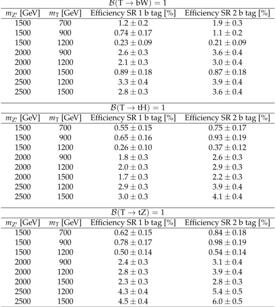
Table 1 shows the selection efficiency for the signal in the different event categories. The sam-ples with the smallest difference in mass between the Z0 boson and T quark have a degraded reconstruction efficiency because of the low pT of the top quark originating from the decay of
the Z0 boson. For several mass points the reconstruction efficiency is higher for the T→tH or T→tZ decay channel than for T→bW, for which the analysis is optimized. This is because if the T quark decays to a t quark instead of a b quark, there are two t quarks in the final state, hence it is more likely that at least one of the two t quarks will be tagged. In addition to this, t quarks coming from the decay of a T quark have a higher pT, therefore are more likely to be
tagged.
5
Background estimation
There are two dominant source of background: multijet QCD production and top quark pro-duction, including both tt and single top quark contributions. The multijet background
contri-6 5 Background estimation
Table 1: Selection efficiencies for the signal in the categories used in the analysis. The quoted uncertainties are statistical.
B(T→bW) =1
mZ0[GeV] mT[GeV] Efficiency SR 1 b tag [%] Efficiency SR 2 b tag [%]
1500 700 1.2±0.2 1.9±0.3 1500 900 0.74±0.17 1.1±0.2 1500 1200 0.23±0.09 0.21±0.09 2000 900 2.6±0.3 3.6±0.4 2000 1200 2.1±0.3 3.0±0.4 2000 1500 0.89±0.18 0.87±0.18 2500 1200 3.3±0.4 3.9±0.4 2500 1500 2.8±0.3 3.6±0.4 B(T→tH) =1
mZ0[GeV] mT[GeV] Efficiency SR 1 b tag [%] Efficiency SR 2 b tag [%]
1500 700 0.55±0.15 0.75±0.17 1500 900 0.65±0.16 0.93±0.19 1500 1200 0.26±0.10 0.37±0.12 2000 900 1.8±0.3 2.6±0.3 2000 1200 2.0±0.3 2.9±0.3 2000 1500 1.7±0.3 2.2±0.3 2500 1200 2.9±0.3 3.9±0.4 2500 1500 3.0±0.3 4.1±0.4 B(T→tZ) =1
mZ0[GeV] mT[GeV] Efficiency SR 1 b tag [%] Efficiency SR 2 b tag [%]
1500 700 0.62±0.15 0.84±0.18 1500 900 0.78±0.17 0.98±0.19 1500 1200 0.50±0.14 0.54±0.14 2000 900 2.4±0.3 3.1±0.4 2000 1200 2.8±0.3 3.9±0.4 2000 1500 2.3±0.3 2.8±0.3 2500 1200 4.3±0.4 5.4±0.5 2500 1500 4.5±0.4 6.0±0.5
bution is the most important for this search. Approximately 20% of the top quark production in the signal region is composed of single top quark events, mostly in the tW channel. Pair pro-duction of top quarks in association with a vector boson is not a relevant background for this analysis because of the non-boosted nature of the process and its relatively small cross section. Its contribution is estimated to be less than 0.3% of the total number of events in the signal region.
The multijet background is derived from data with the following procedure. Sideband regions are defined by inverting the b tagging requirement on the AK4 jet for the selection of the signal. Specifically, the AK4 jet has to fail the b tagging requirement, using a ‘loose’ operating point of the b tagging algorithm. Events with additional b-tagged jets are vetoed to ensure indepen-dence with respect to the signal region. Two different sideband regions are used for the two signal categories according to the presence or absence of a b-tagged subjet in the t-tagged jet. A summary of the selection criteria is shown in Table 2.
The shape of the mZ0 distribution is compared between the sideband region and the signal
region in a sample of simulated multijet QCD events. Figure 2 shows the bin-by-bin ratio of the signal region to the sideband region. Both histograms are normalized to unity before computing the ratio.
Table 2: Summary of the selection criteria for the event categories in the signal region (SR) and the sideband region (SB).
Selection SR 1 b tag SB for 1 b tag SR 2 b tag SB for 2 b tag
1 t tag and 1 W tag Yes Yes Yes Yes
Subjet b tag on t-tagged jet Veto Veto Yes Yes
1 AK4 jet, pT >100 GeV, Yes Yes Yes Yes
∆R(t−/W−jet, jet) >0.8
b tag on AK4 jet Yes “loose” Veto Yes “loose” Veto
mT>500 GeV Yes Yes Yes Yes
[GeV] Z' m 1000 1500 2000 2500 3000 3500 Ratio 0.5 1 1.5 2 2.5 QCD multijet Fit 1 std. deviation ± 1 b-tag category
CMS
Simulation [GeV] Z' m 1000 1500 2000 2500 3000 3500 Ratio 0.5 1 1.5 2 2.5 QCD multijet Fit 1 std. deviation ± 2 b-tag categoryCMS
SimulationFigure 2: Ratio of the number of events in the signal region to the number in the sideband region, as a function of the Z0 mass, for simulated background QCD multijet events. The left (right) plot involves events with no (at least one) b-tagged subjet. The solid line shows a fit of a second-order polynomial function to the ratio.
The ratio is fit with a second-order polynomial function, which represents the correction factor required to weight the events in the sideband region to reproduce the shape of the multijet
8 6 Systematic uncertainties
background in the signal region. This is the simplest functional form providing a satisfactory fit. To avoid double counting when estimating the multijet background from data, the top quark contribution in the sideband region, estimated from simulation, is subtracted. Good agreement in shape between data and simulated events is observed in the sideband regions. The normalization of the predicted multijet background cannot be reliably extracted from sim-ulation and is fixed by a maximum likelihood fit to data in the signal region in a background-only hypothesis. The contribution from tt is properly taken into account. A flat prior is used for the nuisance parameter associated with the normalization of the multijet background. The fit is performed on the mZ0distribution and, as a consistency check, on the HTdistribution,
ob-taining compatible results. It is verified that the scale factor obtained from the fit is not affected by changing the signal hypotheses considered in this analysis. The inclusive normalization factors are 0.093±0.004 and 0.12±0.01 for the 1 and 2 b tag event categories, respectively. This normalization is used for plots in Section 7. For the extraction of upper cross section lim-its on signal production, the normalization of the multijet background is determined by the maximum likelihood fit to data described in Section 7.
The top quark background is estimated using simulated event samples normalized to the the-oretical cross sections, as listed in Section 3. The systematic uncertainties that may impact the event rates and the shapes of the mZ0 and mT distributions in simulated events are discussed
in Section 6. Table 3 shows the expected background yields for the two event categories, along with the observed number of events in data. The uncertainties include both statistical and sys-tematic components; the estimation of the latter is described in Section 6. The yields have been normalized to give the observed total numbers of events.
Table 3: Number of events in the two signal categories of the analysis. The uncertainties include both statistical and systematic components.
Sample SR 1 b tag SR 2 b tag
QCD multijet 1227+−5959 222+−2222 SM top quark 81+−3123 66+−2318 Total background 1308+−6763 288+−3229
Data 1307 289
6
Systematic uncertainties
Several sources of systematic uncertainty may impact the simulated signal and the top quark backgrounds. The procedure used to estimate the multijet background is subject to uncertain-ties as well. These systematic uncertainuncertain-ties affect both the shape and the normalization of the mZ0distribution used in the statistical procedure to infer the presence of signal. The systematic
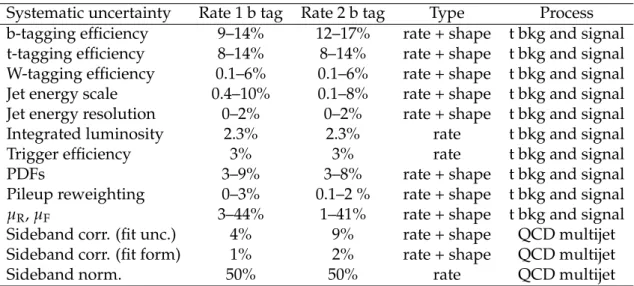
uncertainties are treated as nuisance parameters in the likelihood fit used to extract the upper cross section limit on signal production and are constrained by the data. Table 4 reports the sources of systematic uncertainty, their impact on event rates, the type (rate only, or rate and shape), and the processes for which they are relevant.
The energy scale of jets [52] is corrected with dedicated pT- and η-dependent factors derived
for AK4 and AK8 jets. The jet energy corrections for AK8 subjets are the same as for AK4 jets, scaled for the difference in jet area. Systematic uncertainties are derived by varying the jet energy scale within its uncertainty and thus obtaining the shape and normalization impact on the distribution of mZ0.
Table 4: Sources of systematic uncertainty, their impact on event rates, their type, and the processes for which they are relevant.
Systematic uncertainty Rate 1 b tag Rate 2 b tag Type Process
b-tagging efficiency 9–14% 12–17% rate + shape t bkg and signal
t-tagging efficiency 8–14% 8–14% rate + shape t bkg and signal
W-tagging efficiency 0.1–6% 0.1–6% rate + shape t bkg and signal
Jet energy scale 0.4–10% 0.1–8% rate + shape t bkg and signal
Jet energy resolution 0–2% 0–2% rate + shape t bkg and signal
Integrated luminosity 2.3% 2.3% rate t bkg and signal
Trigger efficiency 3% 3% rate t bkg and signal
PDFs 3–9% 3–8% rate + shape t bkg and signal
Pileup reweighting 0–3% 0.1–2 % rate + shape t bkg and signal
µR, µF 3–44% 1–41% rate + shape t bkg and signal
Sideband corr. (fit unc.) 4% 9% rate + shape QCD multijet
Sideband corr. (fit form) 1% 2% rate + shape QCD multijet
Sideband norm. 50% 50% rate QCD multijet
The energy resolution of jets is lower in data than in simulation, and thus a smearing factor is applied to the four-vectors of AK4 jets, AK8 jets, and to the subjets, in simulated events. The smearing factor for subjets is the same as that for AK4 jets. The impact of this uncertainty, calculated by varying the smearing factor within its uncertainty, is negligible compared to that of the other uncertainties.
The discrepancy of the t tagging efficiency between data and simulation is corrected with scale factors derived in a semileptonic tt topology using a “tag-and-probe” technique [62, 63]. This procedure selects a pure sample of tt events using a tight selection on the leptonically decaying top quark. The sample is then used to measure the efficiency of the t tagging algorithm on the hadronically decaying top quark. The scale factors are derived as a function of the jet pT, along
with their respective uncertainties. A similar procedure is used to derive the correction factors for the W tagging algorithm. Jet and subjet b tagging efficiency correction factors for heavy-and light-flavour jets [60] are varied within their uncertainties to derive the impact on shape and normalization in simulated samples.
Different choices of the renormalization (µR) and factorization (µF) scales used to produce the
simulated samples induce shape and normalization changes in the Z0 boson mass distribution. The impact is assessed by using dedicated simulated top quark and signal events where the µR
and µFare both scaled up or down by a factor of 2.
The pileup reweighting uncertainty is evaluated by varying the effective inelastic cross section by 5%. To account for trigger efficiency discrepancies in data and simulation, a 3% rate uncer-tainty is assigned to the simulated signal and top quark event yields. The unceruncer-tainty in the measurement of the integrated luminosity is calculated to be 2.3% [64].
The systematic uncertainty related to the choice of the PDF values is assessed by varying the eigenvectors for the NNPDF 3.0 set used in the simulation. The variations are summed in quadrature to obtain the shape and rate variation due to PDF effects.
The systematic uncertainty in the estimation of the multijet background arises from the side-band shape correction function (weight function) as explained in Section 5. When fitting the ratio between the sideband and the signal region, the statistical uncertainties of the simulated samples in the procedure are considered. In addition, a linear functional form for the weight function is tested for comparison, and the observed difference is taken into account as a
sys-10 7 Results
tematic uncertainty. These uncertainties are propagated through the background estimation procedure to obtain their impact on the shape and normalization of the mZ0 distribution. The
normalization of the multijet background is determined during the limit setting procedure by allowing it to vary within an uncertainty of 50% in the maximum likelihood fit to data.
The most significant uncertainties are the ones associated with the multijet background fit function, and with the choice of renormalization and factorization scales. Assigning a 50% uncertainty to the multijet background normalization does not significantly affect the results obtained in Section 7.
7
Results
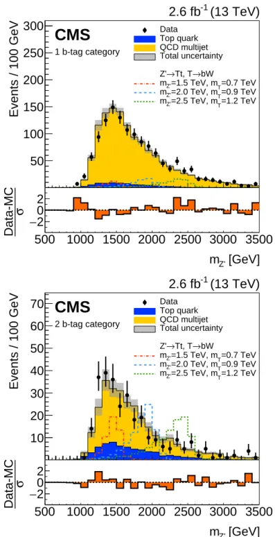
The mZ0distributions in the two signal categories are shown in Fig. 3. The mTand HTvariables
are shown in Fig. 4. No excess with respect to the expected background is observed.
A template-based shape analysis with the THETA software package [65] is performed, using the mZ0distribution in the two categories, to extract upper cross section limits on a hypothetical
signal production. A Bayesian likelihood-based method [27] is used. Expected limit intervals at 95% confidence level (CL) are obtained by performing a large number of pseudo-experiments. The expected background model is varied within the systematic and statistical uncertainties to determine the best fit to the observed data. The modeling of uncertainties in the shapes is performed through cubic-linear template morphing, where the cubic interpolation is used up to one standard deviation and the linear interpolation beyond that [65]. A nuisance parameter is assigned for each systematic uncertainty in the likelihood. For the parameter of interest, i.e. the signal cross section, a uniform prior is used, while log-normal priors are used for the nuisance parameters. The two event categories are fitted simultaneously.
To avoid the normalization of the multijet background being affected by the presence of a hy-pothetical signal, a prior uncertainty of 50% is assigned in the fit of the signal hypothesis, as discussed in Section 5. The fit is able to constrain the multijet normalization, primarily with the 1 b tag category, which has more events and is less signal enriched.
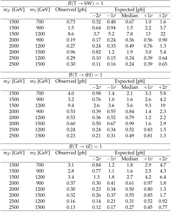
Table 5 shows the expected and observed limits on the cross section to produce a Z0 boson that decays to Tt for different Z0boson and T quark mass hypotheses. Three different hypotheses for the decay of the T quark are considered: 100% branching fraction into bW, tH, or tZ. The effect of increasing the width of the Z0 boson or the T quark to 10% on a single signal configuration has been studied and the impact on the cross section limits is found to be negligible in both cases, because of the detector resolution being bigger than 15%.
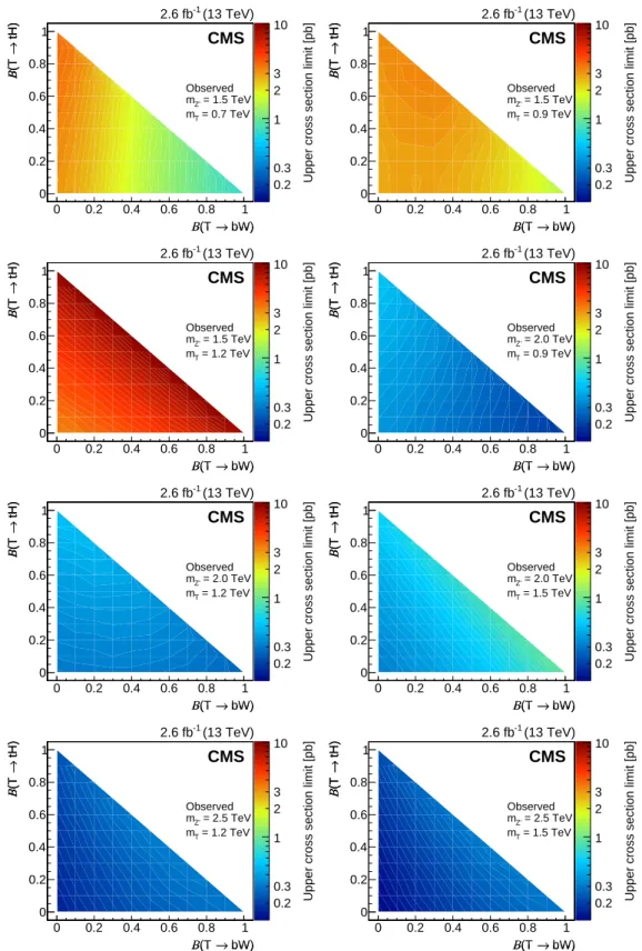
Figures 5 and 6 show the expected and observed upper cross section limits, respectively, for Z0 →Tt for different hypotheses of the Z0boson and T quark masses, and the branching fraction of the T quark into bW and tH channels, withB(T→tZ) = (1− B(T →bW, tH)). Observed cross section limits are in all cases within 2 standard deviations of the expected values.
One-dimensional cross section limits compared to the expectation of the composite Higgs bo-son model [24], as a function of the rebo-sonance mass for mT = 1.2 TeV and T branching fraction
to tH/tZ channels of 50/50%, are shown in Fig. 7 (left). A comparison of the limits to the warped-extra dimension model [22] for T branching fractions to the bW/tH/tZ channels of 50/25/25% is shown on the right-hand side of the same figure. For some values of the mass of the heavy resonance, the resonance width is predicted to be larger than 10% in the bench-mark theoretical models. In these cases the simulated samples do not reproduce the behaviour of the theory benchmarks accurately, hence the cross section values are not considered for the
Events / 100 GeV 50 100 150 200 250 300 Data Top quark QCD multijet Total uncertainty bW → Tt, T → Z' =0.7 TeV T =1.5 TeV, m Z' m =0.9 TeV T =2.0 TeV, m Z' m =1.2 TeV T =2.5 TeV, m Z' m 1 b-tag category
(13 TeV)
-12.6 fb
CMS
[GeV] Z' m 500 1000 1500 2000 2500 3000 3500 σ Data-MC −2 0 2 Events / 100 GeV 10 20 30 40 50 60 70 Data Top quark QCD multijet Total uncertainty bW → Tt, T → Z' =0.7 TeV T =1.5 TeV, m Z' m =0.9 TeV T =2.0 TeV, m Z' m =1.2 TeV T =2.5 TeV, m Z' m 2 b-tag category(13 TeV)
-12.6 fb
CMS
[GeV] Z' m 500 1000 1500 2000 2500 3000 3500 σ Data-MC −2 0 2Figure 3: Distribution of the mZ0 variable for the signal region with 1 b tag (upper plot) and
2 b tags (lower plot) prior to the fit. The yellow (lighter) distribution represents the multi-jet background estimated from data, the blue (darker) distribution is the estimated top quark background, and the black markers are the data. The gray bands represent the statistical and systematic uncertainties in the background estimates. The uncertainty σ includes the statistical uncertainties in data and backgrounds, and the systematic uncertainties in the estimated back-grounds. The dashed lines represent the distributions for signal hypotheses as indicated in the legend. The signal distributions are each normalized to a cross section of 1 pb. Events lying outside the x-axis range are not considered.
12 7 Results Events / 100 GeV 100 200 300 400 500 600 700 Data Top quark QCD multijet Total uncertainty bW → Tt, T → Z' =0.7 TeV T =1.5 TeV, m Z' m =0.9 TeV T =2.0 TeV, m Z' m =1.2 TeV T =2.5 TeV, m Z' m 1 b-tag category (13 TeV) -1 2.6 fb
CMS
[GeV] T m 500 1000 1500 2000 2500 3000 3500 σ Data-MC −2 0 2 Events / 100 GeV 20 40 60 80 100 120 140 160 Data Top quark QCD multijet Total uncertainty bW → Tt, T → Z' =0.7 TeV T =1.5 TeV, m Z' m =0.9 TeV T =2.0 TeV, m Z' m =1.2 TeV T =2.5 TeV, m Z' m 2 b-tag category (13 TeV) -1 2.6 fbCMS
[GeV] T m 500 1000 1500 2000 2500 3000 3500 σ Data-MC −2 0 2 Events / 100 GeV 100 200 300 400500 DataTop quark
QCD multijet Total uncertainty bW → Tt, T → Z' =0.7 TeV T =1.5 TeV, m Z' m =0.9 TeV T =2.0 TeV, m Z' m =1.2 TeV T =2.5 TeV, m Z' m 1 b-tag category (13 TeV) -1 2.6 fb
CMS
[GeV] T H 500 1000 1500 2000 2500 3000 3500 σ Data-MC −2 0 2 Events / 100 GeV 20 40 60 80 100 Data Top quark QCD multijet Total uncertainty bW → Tt, T → Z' =0.7 TeV T =1.5 TeV, m Z' m =0.9 TeV T =2.0 TeV, m Z' m =1.2 TeV T =2.5 TeV, m Z' m 2 b-tag category (13 TeV) -1 2.6 fbCMS
[GeV] T H 500 1000 1500 2000 2500 3000 3500 σ Data-MC −2 0 2Figure 4: Distributions of the mT (upper plots) and HT (lower plots) variables for the 1 b tag
(left) and 2 b tag (right) event categories prior to the fit. The gray bands represent the sta-tistical and systematic uncertainties in the background estimates. The uncertainty σ includes the statistical uncertainties in data and backgrounds, and the systematic uncertainties in the estimated backgrounds. The dashed lines represent the distributions for signal hypotheses as indicated in the legend. The signal distributions are each normalized to a cross section of 1 pb. Events lying outside the x-axis range are not considered.
Table 5: Table of expected and observed limits on the cross section to produce a Z0 boson that decays to Tt at 95% CL for the T →bW (upper), T → tH (middle), and T →tZ (lower) signal hypotheses.
B(T→bW) =1
mZ0 [GeV] mT[GeV] Observed [pb] Expected [pb]
−2σ −1σ Median +1σ +2σ 1500 700 0.73 0.32 0.48 0.67 1.0 1.6 1500 900 1.5 0.64 0.94 1.5 2.2 3.7 1500 1200 8.6 3.7 5.2 7.8 13 22 2000 900 0.19 0.17 0.24 0.36 0.56 0.90 2000 1200 0.27 0.24 0.33 0.49 0.76 1.3 2000 1500 0.96 0.82 1.2 1.9 3.0 5.4 2500 1200 0.29 0.10 0.15 0.24 0.39 0.64 2500 1500 0.30 0.11 0.16 0.24 0.39 0.65 B(T→tH) =1
mZ0 [GeV] mT[GeV] Observed [pb] Expected [pb]
−2σ −1σ Median +1σ +2σ 1500 700 4.0 0.98 1.4 2.1 3.3 5.8 1500 900 3.2 0.76 1.0 1.6 2.6 4.2 1500 1200 9.4 2.6 3.6 5.6 9.3 19 2000 900 0.53 0.39 0.55 0.84 1.4 2.3 2000 1200 0.53 0.36 0.52 0.79 1.2 2.2 2000 1500 0.60 0.50 0.67 0.99 1.6 2.9 2500 1200 0.24 0.24 0.34 0.52 0.83 1.5 2500 1500 0.23 0.21 0.31 0.49 0.81 1.3 B(T→tZ) =1
mZ0 [GeV] mT[GeV] Observed [pb] Expected [pb]
−2σ −1σ Median +1σ +2σ 1500 700 3.1 0.84 1.2 1.8 2.9 4.7 1500 900 2.8 0.77 1.1 1.6 2.5 4.3 1500 1200 3.4 1.3 1.8 2.7 4.2 6.4 2000 900 0.37 0.30 0.41 0.61 0.97 1.8 2000 1200 0.30 0.23 0.34 0.50 0.80 1.3 2000 1500 0.32 0.26 0.37 0.55 0.85 1.7 2500 1200 0.16 0.14 0.21 0.31 0.52 0.92 2500 1500 0.13 0.12 0.17 0.27 0.45 0.77
14 7 Results bW) → (T Β 0 0.2 0.4 0.6 0.8 1 tH) → (T Β 0 0.2 0.4 0.6 0.8 1
Upper cross section limit [pb]
0.2 0.3 1 2 3 10 bW) → (T Β 0 0.2 0.4 0.6 0.8 1 tH) → (T Β 0 0.2 0.4 0.6 0.8 1 (13 TeV) -1 2.6 fb CMS Simulation = 0.7 TeV T m = 1.5 TeV Z' m Expected bW) → (T Β 0 0.2 0.4 0.6 0.8 1 tH) → (T Β 0 0.2 0.4 0.6 0.8 1
Upper cross section limit [pb]
0.2 0.3 1 2 3 10 bW) → (T Β 0 0.2 0.4 0.6 0.8 1 tH) → (T Β 0 0.2 0.4 0.6 0.8 1 (13 TeV) -1 2.6 fb CMS Simulation = 0.9 TeV T m = 1.5 TeV Z' m Expected bW) → (T Β 0 0.2 0.4 0.6 0.8 1 tH) → (T Β 0 0.2 0.4 0.6 0.8 1
Upper cross section limit [pb]
0.2 0.3 1 2 3 10 bW) → (T Β 0 0.2 0.4 0.6 0.8 1 tH) → (T Β 0 0.2 0.4 0.6 0.8 1 (13 TeV) -1 2.6 fb CMS Simulation = 1.2 TeV T m = 1.5 TeV Z' m Expected bW) → (T Β 0 0.2 0.4 0.6 0.8 1 tH) → (T Β 0 0.2 0.4 0.6 0.8 1
Upper cross section limit [pb]
0.2 0.3 1 2 3 10 bW) → (T Β 0 0.2 0.4 0.6 0.8 1 tH) → (T Β 0 0.2 0.4 0.6 0.8 1 (13 TeV) -1 2.6 fb CMS Simulation = 0.9 TeV T m = 2.0 TeV Z' m Expected bW) → (T Β 0 0.2 0.4 0.6 0.8 1 tH) → (T Β 0 0.2 0.4 0.6 0.8 1
Upper cross section limit [pb]
0.2 0.3 1 2 3 10 bW) → (T Β 0 0.2 0.4 0.6 0.8 1 tH) → (T Β 0 0.2 0.4 0.6 0.8 1 (13 TeV) -1 2.6 fb CMS Simulation = 1.2 TeV T m = 2.0 TeV Z' m Expected bW) → (T Β 0 0.2 0.4 0.6 0.8 1 tH) → (T Β 0 0.2 0.4 0.6 0.8 1
Upper cross section limit [pb]
0.2 0.3 1 2 3 10 bW) → (T Β 0 0.2 0.4 0.6 0.8 1 tH) → (T Β 0 0.2 0.4 0.6 0.8 1 (13 TeV) -1 2.6 fb CMS Simulation = 1.5 TeV T m = 2.0 TeV Z' m Expected bW) → (T Β 0 0.2 0.4 0.6 0.8 1 tH) → (T Β 0 0.2 0.4 0.6 0.8 1
Upper cross section limit [pb]
0.2 0.3 1 2 3 10 bW) → (T Β 0 0.2 0.4 0.6 0.8 1 tH) → (T Β 0 0.2 0.4 0.6 0.8 1 (13 TeV) -1 2.6 fb CMS Simulation = 1.2 TeV T m = 2.5 TeV Z' m Expected bW) → (T Β 0 0.2 0.4 0.6 0.8 1 tH) → (T Β 0 0.2 0.4 0.6 0.8 1
Upper cross section limit [pb]
0.2 0.3 1 2 3 10 bW) → (T Β 0 0.2 0.4 0.6 0.8 1 tH) → (T Β 0 0.2 0.4 0.6 0.8 1 (13 TeV) -1 2.6 fb CMS Simulation = 1.5 TeV T m = 2.5 TeV Z' m Expected
Figure 5: Expected cross section limits for Z0 → Tt for different hypotheses for the Z0 boson and T quark masses, and the branching fraction of the T quark decay into bW and tH channels,
bW) → (T Β 0 0.2 0.4 0.6 0.8 1 tH) → (T Β 0 0.2 0.4 0.6 0.8 1
Upper cross section limit [pb]
0.2 0.3 1 2 3 10 bW) → (T Β 0 0.2 0.4 0.6 0.8 1 tH) → (T Β 0 0.2 0.4 0.6 0.8 1 (13 TeV) -1 2.6 fb CMS = 0.7 TeV T m = 1.5 TeV Z' m Observed bW) → (T Β 0 0.2 0.4 0.6 0.8 1 tH) → (T Β 0 0.2 0.4 0.6 0.8 1
Upper cross section limit [pb]
0.2 0.3 1 2 3 10 bW) → (T Β 0 0.2 0.4 0.6 0.8 1 tH) → (T Β 0 0.2 0.4 0.6 0.8 1 (13 TeV) -1 2.6 fb CMS = 0.9 TeV T m = 1.5 TeV Z' m Observed bW) → (T Β 0 0.2 0.4 0.6 0.8 1 tH) → (T Β 0 0.2 0.4 0.6 0.8 1
Upper cross section limit [pb]
0.2 0.3 1 2 3 10 bW) → (T Β 0 0.2 0.4 0.6 0.8 1 tH) → (T Β 0 0.2 0.4 0.6 0.8 1 (13 TeV) -1 2.6 fb CMS = 1.2 TeV T m = 1.5 TeV Z' m Observed bW) → (T Β 0 0.2 0.4 0.6 0.8 1 tH) → (T Β 0 0.2 0.4 0.6 0.8 1
Upper cross section limit [pb]
0.2 0.3 1 2 3 10 bW) → (T Β 0 0.2 0.4 0.6 0.8 1 tH) → (T Β 0 0.2 0.4 0.6 0.8 1 (13 TeV) -1 2.6 fb CMS = 0.9 TeV T m = 2.0 TeV Z' m Observed bW) → (T Β 0 0.2 0.4 0.6 0.8 1 tH) → (T Β 0 0.2 0.4 0.6 0.8 1
Upper cross section limit [pb]
0.2 0.3 1 2 3 10 bW) → (T Β 0 0.2 0.4 0.6 0.8 1 tH) → (T Β 0 0.2 0.4 0.6 0.8 1 (13 TeV) -1 2.6 fb CMS = 1.2 TeV T m = 2.0 TeV Z' m Observed bW) → (T Β 0 0.2 0.4 0.6 0.8 1 tH) → (T Β 0 0.2 0.4 0.6 0.8 1
Upper cross section limit [pb]
0.2 0.3 1 2 3 10 bW) → (T Β 0 0.2 0.4 0.6 0.8 1 tH) → (T Β 0 0.2 0.4 0.6 0.8 1 (13 TeV) -1 2.6 fb CMS = 1.5 TeV T m = 2.0 TeV Z' m Observed bW) → (T Β 0 0.2 0.4 0.6 0.8 1 tH) → (T Β 0 0.2 0.4 0.6 0.8 1
Upper cross section limit [pb]
0.2 0.3 1 2 3 10 bW) → (T Β 0 0.2 0.4 0.6 0.8 1 tH) → (T Β 0 0.2 0.4 0.6 0.8 1 (13 TeV) -1 2.6 fb CMS = 1.2 TeV T m = 2.5 TeV Z' m Observed bW) → (T Β 0 0.2 0.4 0.6 0.8 1 tH) → (T Β 0 0.2 0.4 0.6 0.8 1
Upper cross section limit [pb]
0.2 0.3 1 2 3 10 bW) → (T Β 0 0.2 0.4 0.6 0.8 1 tH) → (T Β 0 0.2 0.4 0.6 0.8 1 (13 TeV) -1 2.6 fb CMS = 1.5 TeV T m = 2.5 TeV Z' m Observed
Figure 6: Observed cross section limits for Z0 → Tt for different hypotheses for the Z0 boson and T quark masses, and the branching fraction of the T quark decay into bW and tH channels,
16 8 Summary
comparison and are marked by a dashed line in Fig. 7. The increase of the total width of the resonance with the increase of its mass is caused by additional decay channels becoming kine-matically allowed. The change in slope of the theoretical cross sections around mZ0 = 1.6 and
2.4 TeV is due to the Tt and TT decay channels respectively becoming kinematically allowed. The comparison with the expectations of theoretical models shows that this search has no sen-sitivity to the composite Higgs model [24] and some sensen-sitivity to the extra dimensions model [22], however more data is needed to exclude specific scenarios.
mass [TeV] L
0
ρ
1.4 1.6 1.8 2 2.2 2.4 2.6
Upper cross section limit [pb]
3 − 10 2 − 10 1 − 10 1 10 2 10 3 10 4 10 Β(T→ tH, tZ) = 50%, 50% Observed Expected 1 std. deviation ± 2 std. deviation ± = 3 L ρ = 1, g 3 = c 2 = c L Tt, y → L 0 ρ > 10 % L 0 ρ /m L 0 ρ Γ (13 TeV) -1 2.6 fb
CMS
G* mass [TeV] 1.4 1.6 1.8 2 2.2 2.4 2.6Upper cross section limit [pb]
2 − 10 1 − 10 1 10 2 10 3 10 4 10 Β(T→ bW, tH, tZ) = 50%, 25%, 25% Observed Expected 1 std. deviation ± 2 std. deviation ± = 3 * = 0.6, Y tR φ = 0.44, sin 3 θ Tt, tan → G* > 10 % G* /m G* Γ (13 TeV) -1 2.6 fb
CMS
Figure 7: One-dimensional cross section limits at 95% CL as a function of the heavy vector resonance mass for mT = 1.2 TeV, assuming branching fractions of the T quark decay to the
tH/tZ channels of 50/50% (left) or to the bW/tH/tZ channels of 50/25/25% (right). The solid line is the observed limit, the dotted line is the expected limit, shown with 68% (inner) and 95% (outer) uncertainty bands. In the left plot, the green thick line is the product of the cross section and branching fraction for a heavy spin-1 resonance ρ0L → Tt in a composite Higgs boson model [24]. In the right plot, the blue thick line is the product of the cross section and branching fraction for a heavy gluon G∗ → Tt in a warped extra-dimension model [22]. The theoretical predictions are shown as dashed lines where the width of the resonance is larger than 10% of its mass.
8
Summary
A search for a massive spin-1 resonance decaying to a top quark and a vector-like T quark has been performed in the all-jets channel using √s = 13 TeV proton-proton collision data collected by CMS at the LHC. The search uses jet-substructure techniques, involving top quark and W boson tagging algorithms, along with subjet b tagging. The top quark and W boson algorithms are based on the N-subjettiness variables and use the modified mass-drop algorithm to compute the jet mass. The multijet background is estimated in data through a sideband region that is adjusted through simulation-based correction factors. The top quark background is estimated using simulated events.
No excess is observed in data beyond the standard model expectations, and upper limits are set on the production cross sections of hypothetical signals. The cross section limits are com-pared to the cross sections of a spin-1 resonance in a composite Higgs boson model and a Kaluza-Klein gluon in a warped extra-dimension model, for benchmark values of the model parameters, assuming a T quark mass of 1.2 TeV. Branching fractions of the T quark decay to the tH/tZ channels of 50/50% and to the bW/tH/tZ channels of 50/25/25% are assumed for
models with a composite Higgs boson and with a warped extra-dimension, respectively. This search is not sensitive to the composite Higgs model [24] with the analyzed data. In the case of the model with a warped extra-dimension [22], the upper limit obtained on the cross section is just at the predicted level for G∗masses in the region of 1.8 TeV. Although limits are not placed on these particular models, more generally a Z0 boson decaying to a top and a T quark is ex-cluded at 95% confidence level, with upper limits on production cross sections ranging from 0.13 to 10 pb, depending on the hypotheses. This is the first search for a heavy spin-1 resonance decaying to a vector-like T quark and a top quark.
Acknowledgments
We congratulate our colleagues in the CERN accelerator departments for the excellent perfor-mance of the LHC and thank the technical and administrative staffs at CERN and at other CMS institutes for their contributions to the success of the CMS effort. In addition, we grate-fully acknowledge the computing centres and personnel of the Worldwide LHC Computing Grid for delivering so effectively the computing infrastructure essential to our analyses. Fi-nally, we acknowledge the enduring support for the construction and operation of the LHC and the CMS detector provided by the following funding agencies: BMWFW and FWF (Aus-tria); FNRS and FWO (Belgium); CNPq, CAPES, FAPERJ, and FAPESP (Brazil); MES (Bulgaria); CERN; CAS, MoST, and NSFC (China); COLCIENCIAS (Colombia); MSES and CSF (Croatia); RPF (Cyprus); SENESCYT (Ecuador); MoER, ERC IUT, and ERDF (Estonia); Academy of Fin-land, MEC, and HIP (Finland); CEA and CNRS/IN2P3 (France); BMBF, DFG, and HGF (Ger-many); GSRT (Greece); OTKA and NIH (Hungary); DAE and DST (India); IPM (Iran); SFI (Ireland); INFN (Italy); MSIP and NRF (Republic of Korea); LAS (Lithuania); MOE and UM (Malaysia); BUAP, CINVESTAV, CONACYT, LNS, SEP, and UASLP-FAI (Mexico); MBIE (New Zealand); PAEC (Pakistan); MSHE and NSC (Poland); FCT (Portugal); JINR (Dubna); MON, RosAtom, RAS, RFBR and RAEP (Russia); MESTD (Serbia); SEIDI, CPAN, PCTI and FEDER (Spain); Swiss Funding Agencies (Switzerland); MST (Taipei); ThEPCenter, IPST, STAR, and NSTDA (Thailand); TUBITAK and TAEK (Turkey); NASU and SFFR (Ukraine); STFC (United Kingdom); DOE and NSF (USA).
Individuals have received support from the Marie-Curie programme and the European Re-search Council and EPLANET (European Union); the Leventis Foundation; the A. P. Sloan Foundation; the Alexander von Humboldt Foundation; the Belgian Federal Science Policy Of-fice; the Fonds pour la Formation `a la Recherche dans l’Industrie et dans l’Agriculture (FRIA-Belgium); the Agentschap voor Innovatie door Wetenschap en Technologie (IWT-(FRIA-Belgium); the Ministry of Education, Youth and Sports (MEYS) of the Czech Republic; the Council of Sci-ence and Industrial Research, India; the HOMING PLUS programme of the Foundation for Polish Science, cofinanced from European Union, Regional Development Fund, the Mobil-ity Plus programme of the Ministry of Science and Higher Education, the National Science Center (Poland), contracts Harmonia 2014/14/M/ST2/00428, Opus 2014/13/B/ST2/02543, 2014/15/B/ST2/03998, and 2015/19/B/ST2/02861, Sonata-bis 2012/07/E/ST2/01406; the Na-tional Priorities Research Program by Qatar NaNa-tional Research Fund; the Programa Clar´ın-COFUND del Principado de Asturias; the Thalis and Aristeia programmes cofinanced by EU-ESF and the Greek NSRF; the Rachadapisek Sompot Fund for Postdoctoral Fellowship, Chula-longkorn University and the ChulaChula-longkorn Academic into Its 2nd Century Project Advance-ment Project (Thailand); and the Welch Foundation, contract C-1845.
18 References
References
[1] S. Dimopoulos and H. Georgi, “Softly broken supersymmetry and SU(5)”, Nucl. Phys. B
193(1981) 150, doi:10.1016/0550-3213(81)90522-8.
[2] S. Weinberg, “Implications of dynamical symmetry breaking”, Phys. Rev. D 13 (1976) 974, doi:10.1103/PhysRevD.13.974.
[3] L. Susskind, “Dynamics of spontaneous symmetry breaking in the Weinberg-Salam theory”, Phys. Rev. D 20 (1979) 2619, doi:10.1103/PhysRevD.20.2619.
[4] C. T. Hill and S. J. Parke, “Top production: Sensitivity to new physics”, Phys. Rev. D 49 (1994) 4454, doi:10.1103/PhysRevD.49.4454, arXiv:hep-ph/9312324.
[5] R. S. Chivukula, B. A. Dobrescu, H. Georgi, and C. T. Hill, “Top quark seesaw theory of electroweak symmetry breaking”, Phys. Rev. D 59 (1999) 075003,
doi:10.1103/PhysRevD.59.075003, arXiv:hep-ph/9809470.
[6] N. Arkani-Hamed, A. G. Cohen, and H. Georgi, “Electroweak symmetry breaking from dimensional deconstruction”, Phys. Lett. B 513 (2001) 232,
doi:10.1016/S0370-2693(01)00741-9, arXiv:hep-ph/0105239.
[7] N. Arkani-Hamed, S. Dimopoulos, and G. R. Dvali, “The hierarchy problem and new dimensions at a millimeter”, Phys. Lett. B 429 (1998) 263,
doi:10.1016/S0370-2693(98)00466-3, arXiv:hep-ph/9803315.
[8] L. Randall and R. Sundrum, “A Large Mass Hierarchy from a Small Extra Dimension”, Phys. Rev. Lett. 83 (1999) 3370, doi:10.1103/PhysRevLett.83.3370,
arXiv:hep-ph/9905221.
[9] L. Randall and R. Sundrum, “An Alternative to Compactification”, Phys. Rev. Lett. 83 (1999) 4690, doi:10.1103/PhysRevLett.83.4690, arXiv:hep-th/9906064. [10] J. L. Rosner, “Prominent decay modes of a leptophobic Z’”, Phys. Rev. B 387 (1996) 113,
doi:10.1016/0370-2693(96)01022-2, arXiv:hep-ph/9607207v3. [11] C. T. Hill, “Topcolor assisted technicolor”, Phys. Lett. B 345 (1995) 483,
doi:10.1016/0370-2693(94)01660-5, arXiv:hep-ph/9411426. Updates in arXiv:hep-ph/9911288.
[12] K. R. Lynch, M. Narain, E. H. Simmons, and S. Mrenna, “Finding Z’ bosons coupled preferentially to the third family at CERN LEP and the Fermilab Tevatron”, Phys. Rev. D
63(2001) 035006, doi:10.1103/PhysRevD.63.035006, arXiv:hep-ph/0007286.
[13] K. Agashe et al., “LHC signals for warped electroweak neutral gauge bosons”, Phys. Rev. D 76 (2007) 115015, doi:10.1103/PhysRevD.80.075007, arXiv:0810.1497. [14] K. Agashe et al., “LHC signals from warped extra dimensions”, Phys. Rev. D 77 (2008)
015003, doi:10.1103/PhysRevD.77.015003, arXiv:hep-ph/0612015. [15] CMS Collaboration, “Search for anomalous tt production in the highly-boosed
all-hadronic final state”, JHEP 09 (2012) 29, doi:10.1007/JHEP09(2012)029, arXiv:1204.2488.
[16] CMS Collaboration, “Search for resonant tt production in lepton+jets events in pp
collisions at√s = 7 TeV”, JHEP 12 (2012) 15, doi:10.1007/JHEP12(2012)015,
arXiv:1209.4397.
[17] ATLAS Collaboration, “Search for resonances decaying into top-quark pairs using fully hadronic decays in pp collisions with ATLAS at√s = 7 TeV”, JHEP 01 (2013) 116, doi:10.1007/JHEP01(2013)116, arXiv:1211.2202.
[18] ATLAS Collaboration, “A search for tt resonances in lepton+jets events with
highly-boosed top quarks collected in pp collisions with ATLAS at√s = 7 TeV”, JHEP 09 (2012) 41, doi:10.1007/JHEP09(2012)041, arXiv:1207.2409.
[19] CMS Collaboration, “Searches for New Physics Using the t¯t Invariant Mass Distribution in pp Collisions at√s =8 TeV”, Phys. Rev. Lett. 111 (2013) 211804,
doi:10.1103/PhysRevLett.111.211804, arXiv:1309.2030.
[20] CMS Collaboration, “Search for resonant tt production in proton-proton collisions at√s = 8 TeV”, Phys. Rev. D 93 (2016) 012001, doi:10.1103/PhysRevD.93.012001,
arXiv:1506.03062.
[21] ATLAS Collaboration, “A search for tt resonances using lepton-plus-jets events in proton-proton collisions at√s = 8 TeV with the ATLAS detector”, JHEP 08 (2015) 148, doi:10.1007/JHEP08(2015)148, arXiv:1505.07018.
[22] C. Bini, R. Contino, and N. Vignaroli, “Heavy-light decay topologies as a new strategy to discover a heavy gluon”, JHEP 01 (2012) 157, doi:10.1007/JHEP01(2012)157, arXiv:1110.6058.
[23] B. A. Dobrescu, K. Kong, and R. Mahbubani, “Prospects for top-prime quark discovery at the Tevatron”, JHEP 06 (2009) 001, doi:10.1088/1126-6708/2009/06/001,
arXiv:0902.0792.
[24] D. Greco and D. Liu, “Hunting composite vector resonances at the LHC: naturalness facing data”, JHEP 12 (2014) 126, doi:10.1007/JHEP12(2014)126,
arXiv:1410.2883.
[25] N. Vignaroli, “New W’ signals at the LHC”, Phys. Rev. D 89 (2014) 095027, doi:10.1103/PhysRevD.89.095027, arXiv:1404.5558.
[26] ATLAS, CMS Collaboration, “Measurements of the Higgs boson production and decay rates and constraints on its couplings from a combined ATLAS and CMS analysis of the LHC pp collision data at√s =7 and 8 TeV”, JHEP 08 (2016) 045,
doi:10.1007/JHEP08(2016)045, arXiv:1606.02266.
[27] Particle Data Group Collaboration, “Review of Particle Physics”, Chin. Phys. C 40 (2016), no. 10, 100001, doi:10.1088/1674-1137/40/10/100001.
[28] CMS Collaboration, “Particle-flow event reconstruction in CMS and performance for jets, taus, and EmissT ”, CMS Physics Analysis Summary CMS-PAS-PFT-09-001, CERN, 2009. [29] CMS Collaboration, “Commissioning of the particle-flow event reconstruction with the
first LHC collisions recorded in the CMS detector”, CMS Physics Analysis Summary CMS-PAS-PFT-10-001, CERN, 2010.
20 References
[30] CMS Collaboration, “Description and performance of track and primary-vertex reconstruction with the CMS tracker”, JINST 9 (2014) P10009,
doi:10.1088/1748-0221/9/10/P10009, arXiv:1405.6569.
[31] CMS Collaboration, “The CMS experiment at the CERN LHC”, JINST 3 (2008) S08004,
doi:10.1088/1748-0221/3/08/S08004.
[32] J. Alwall et al., “The automated computation of tree-level and next-to-leading order differential cross sections, and their matching to parton shower simulations”, JHEP 07 (2014) 079, doi:10.1007/JHEP07(2014)079, arXiv:1405.0301.
[33] P. Artoisenet, R. Frederix, O. Mattelaer, and R. Rietkerk, “Automatic spin-entangled decays of heavy resonances in Monte Carlo simulations”, JHEP 03 (2013) 015,
doi:10.1007/JHEP03(2013)015, arXiv:1212.3460.
[34] T. Sj ¨ostrand et al., “An introduction to PYTHIA 8.2”, Comput. Phys. Commun. 191 (2015) 159, doi:10.1016/j.cpc.2015.01.024, arXiv:1410.3012.
[35] CMS Collaboration, “Event generator tunes obtained from underlying event and multiparton scattering measurements”, Eur. Phys. J. C 76 (2016) 155,
doi:10.1140/epjc/s10052-016-3988-x, arXiv:1512.00815.
[36] M. L. Mangano, M. Moretti, F. Piccinini, and M. Treccani, “Matching matrix elements and shower evolution for top-quark production in hadronic collisions”, JHEP 01 (2007) 013,
doi:10.1088/1126-6708/2007/01/013, arXiv:hep-ph/0611129.
[37] P. Nason, “A new method for combining NLO QCD with shower Monte Carlo algorithms”, JHEP 11 (2004) 040, doi:10.1088/1126-6708/2004/11/040,
arXiv:hep-ph/0409146.
[38] S. Frixione, P. Nason, and C. Oleari, “Matching NLO QCD computations with parton shower simulations: the POWHEG method”, JHEP 11 (2007) 070,
doi:10.1088/1126-6708/2007/11/070, arXiv:0709.2092.
[39] S. Alioli, P. Nason, C. Oleari, and E. Re, “A general framework for implementing NLO calculations in shower Monte Carlo programs: the POWHEG BOX”, JHEP 06 (2010) 043, doi:10.1007/JHEP06(2010)043, arXiv:1002.2581.
[40] S. Frixione, P. Nason, and G. Ridolfi, “A positive-weight next-to-leading-order Monte Carlo for heavy flavour hadroproduction”, JHEP 09 (2007) 126,
doi:10.1088/1126-6708/2007/09/126, arXiv:0707.3088.
[41] E. Re, “Single-top Wt-channel production matched with parton showers using the POWHEG method”, Eur. Phys. J. C 71 (2011) 1547,
doi:10.1140/epjc/s10052-011-1547-z, arXiv:1009.2450.
[42] M. Czakon and A. Mitov, “Top++: a program for the calculation of the top-pair cross-section at hadron colliders”, Comput. Phys. Commun. 185 (2014) 2930,
doi:10.1016/j.cpc.2014.06.021, arXiv:1112.5675.
[43] N. Kidonakis, “Two-loop soft anomalous dimensions for single top quark associated production with a W−or H−”, Phys. Rev. D 82 (2010) 054018,
doi:10.1103/PhysRevD.82.054018, arXiv:1005.4451. Updates in
[44] M. Aliev et al., “HATHOR: HAdronic Top and Heavy quarks crOss section calculatoR”, Comput. Phys. Commun. 182 (2011) 1034, doi:10.1016/j.cpc.2010.12.040, arXiv:1007.1327.
[45] P. Kant et al., “HatHor for single top-quark production: Updated predictions and uncertainty estimates for single top-quark production in hadronic collisions”, Comput. Phys. Commun. 191 (2015) 74, doi:10.1016/j.cpc.2015.02.001,
arXiv:1406.4403.
[46] NNPDF Collaboration, “Parton distributions for the LHC Run II”, JHEP 04 (2015) 040,
doi:10.1007/JHEP04(2015)040, arXiv:1410.8849.
[47] GEANT4 Collaboration, “GEANT4—a simulation toolkit”, Nucl. Instrum. Meth. A 506 (2003) 250, doi:10.1016/S0168-9002(03)01368-8.
[48] J. Allison et al., “Geant4 developments and applications”, IEEE Trans. Nucl. Sci. 53 (2006) 270, doi:10.1109/TNS.2006.869826.
[49] M. Cacciari, G. P. Salam, and G. Soyez, “The anti-ktjet clustering algorithm”, JHEP 04
(2008) 063, doi:10.1088/1126-6708/2008/04/063, arXiv:0802.1189.
[50] M. Cacciari and G. P. Salam, “Dispelling the N3myth for the ktjet-finder”, Phys. Lett. B
641(2006) 57, doi:10.1016/j.physletb.2006.08.037, arXiv:hep-ph/0512210.
[51] M. Cacciari and G. P. Salam, “Pileup subtraction using jet areas”, Phys. Lett. B 659 (2008) 119, doi:10.1016/j.physletb.2007.09.077, arXiv:0707.1378.
[52] CMS Collaboration, “Determination of Jet Energy Calibration and Transverse Momentum Resolution in CMS”, JINST 6 (2011) P11002,
doi:10.1088/1748-0221/6/11/P11002, arXiv:1107.4277.
[53] CMS Collaboration, “Top Tagging with New Approaches”, CMS Physics Analysis Summary CMS-PAS-JME-15-002, CERN, 2016.
[54] Y. L. Dokshitzer, G. D. Leder, S. Moretti, and B. R. Webber, “Better jet clustering algorithms”, JHEP 08 (1997) 001, doi:10.1088/1126-6708/1997/08/001,
arXiv:hep-ph/9707323.
[55] M. Wobisch and T. Wengler, “Hadronization corrections to jet cross-sections in deep-inelastic scattering”, (1998). arXiv:hep-ph/9907280.
[56] M. Dasgupta, A. Fregoso, S. Marzani, and G. P. Salam, “Towards an understanding of jet substructure”, JHEP 09 (2013) 029, doi:10.1007/JHEP09(2013)029,
arXiv:1307.0007.
[57] A. J. Larkoski, S. Marzani, G. Soyez, and J. Thaler, “Soft drop”, JHEP 05 (2014) 146,
doi:10.1007/JHEP05(2014)146, arXiv:1402.2657.
[58] J. Thaler and K. Van Tilburg, “Identifying boosted objects with N-subjettiness”, JHEP 03 (2011) 015, doi:10.1007/JHEP03(2011)015, arXiv:1011.2268.
[59] J. Thaler and K. Van Tilburg, “Maximizing boosted top identification by minimizing N-subjettiness”, JHEP 02 (2012) 093, doi:10.1007/JHEP02(2012)093,
22 References
[60] CMS Collaboration, “Identification of b quark jets at the CMS Experiment in the LHC Run 2”, CMS Physics Analysis Summary CMS-PAS-BTV-15-001, CERN, 2016.
[61] CMS Collaboration, “Identification of b-quark jets with the CMS experiment”, JINST 8 (2013) P04013, doi:10.1088/1748-0221/8/04/P04013, arXiv:1211.4462. [62] CMS Collaboration, “Boosted Top Jet Tagging at CMS”, CMS Physics Analysis Summary
CMS-PAS-JME-13-007, CERN, 2014.
[63] CMS Collaboration, “Measurements of inclusive W and Z cross sections in pp collisions
at√s=7 TeV”, JHEP 01 (2011) 080, doi:10.1007/JHEP01(2011)080,
arXiv:1012.2466.
[64] CMS Collaboration, “CMS Luminosity Measurement for the 2015 Data Taking Period”, CMS Physics Analysis Summary CMS-PAS-LUM-15-001, CERN, 2016.
[65] T. M ¨uller, J. Ott, and J. Wagner-Kuhr, “Theta – a framework for template-based modeling and inference”, 2010,
A
The CMS Collaboration
Yerevan Physics Institute, Yerevan, Armenia A.M. Sirunyan, A. Tumasyan
Institut f ¨ur Hochenergiephysik, Wien, Austria
W. Adam, E. Asilar, T. Bergauer, J. Brandstetter, E. Brondolin, M. Dragicevic, J. Er ¨o, M. Flechl, M. Friedl, R. Fr ¨uhwirth1, V.M. Ghete, C. Hartl, N. H ¨ormann, J. Hrubec, M. Jeitler1, A. K ¨onig, I. Kr¨atschmer, D. Liko, T. Matsushita, I. Mikulec, D. Rabady, N. Rad, B. Rahbaran, H. Rohringer, J. Schieck1, J. Strauss, W. Waltenberger, C.-E. Wulz1
Institute for Nuclear Problems, Minsk, Belarus
O. Dvornikov, V. Makarenko, V. Mossolov, J. Suarez Gonzalez, V. Zykunov National Centre for Particle and High Energy Physics, Minsk, Belarus N. Shumeiko
Universiteit Antwerpen, Antwerpen, Belgium
S. Alderweireldt, E.A. De Wolf, X. Janssen, J. Lauwers, M. Van De Klundert, H. Van Haevermaet, P. Van Mechelen, N. Van Remortel, A. Van Spilbeeck
Vrije Universiteit Brussel, Brussel, Belgium
S. Abu Zeid, F. Blekman, J. D’Hondt, N. Daci, I. De Bruyn, K. Deroover, S. Lowette, S. Moortgat, L. Moreels, A. Olbrechts, Q. Python, K. Skovpen, S. Tavernier, W. Van Doninck, P. Van Mulders, I. Van Parijs
Universit´e Libre de Bruxelles, Bruxelles, Belgium
H. Brun, B. Clerbaux, G. De Lentdecker, H. Delannoy, G. Fasanella, L. Favart, R. Goldouzian, A. Grebenyuk, G. Karapostoli, T. Lenzi, A. L´eonard, J. Luetic, T. Maerschalk, A. Marinov, A. Randle-conde, T. Seva, C. Vander Velde, P. Vanlaer, D. Vannerom, R. Yonamine, F. Zenoni, F. Zhang2
Ghent University, Ghent, Belgium
A. Cimmino, T. Cornelis, D. Dobur, A. Fagot, M. Gul, I. Khvastunov, D. Poyraz, S. Salva, R. Sch ¨ofbeck, M. Tytgat, W. Van Driessche, E. Yazgan, N. Zaganidis
Universit´e Catholique de Louvain, Louvain-la-Neuve, Belgium
H. Bakhshiansohi, C. Beluffi3, O. Bondu, S. Brochet, G. Bruno, A. Caudron, S. De Visscher, C. Delaere, M. Delcourt, B. Francois, A. Giammanco, A. Jafari, M. Komm, G. Krintiras, V. Lemaitre, A. Magitteri, A. Mertens, M. Musich, K. Piotrzkowski, L. Quertenmont, M. Selvaggi, M. Vidal Marono, S. Wertz
Universit´e de Mons, Mons, Belgium N. Beliy
Centro Brasileiro de Pesquisas Fisicas, Rio de Janeiro, Brazil
W.L. Ald´a J ´unior, F.L. Alves, G.A. Alves, L. Brito, C. Hensel, A. Moraes, M.E. Pol, P. Rebello Teles
Universidade do Estado do Rio de Janeiro, Rio de Janeiro, Brazil
E. Belchior Batista Das Chagas, W. Carvalho, J. Chinellato4, A. Cust ´odio, E.M. Da Costa,
G.G. Da Silveira5, D. De Jesus Damiao, C. De Oliveira Martins, S. Fonseca De Souza,
L.M. Huertas Guativa, H. Malbouisson, D. Matos Figueiredo, C. Mora Herrera, L. Mundim, H. Nogima, W.L. Prado Da Silva, A. Santoro, A. Sznajder, E.J. Tonelli Manganote4, F. Torres Da Silva De Araujo, A. Vilela Pereira
24 A The CMS Collaboration
Universidade Estadual Paulistaa, Universidade Federal do ABCb, S˜ao Paulo, Brazil
S. Ahujaa, C.A. Bernardesa, S. Dograa, T.R. Fernandez Perez Tomeia, E.M. Gregoresb, P.G. Mercadanteb, C.S. Moona, S.F. Novaesa, Sandra S. Padulaa, D. Romero Abadb, J.C. Ruiz Vargasa
Institute for Nuclear Research and Nuclear Energy, Sofia, Bulgaria
A. Aleksandrov, R. Hadjiiska, P. Iaydjiev, M. Rodozov, S. Stoykova, G. Sultanov, M. Vutova University of Sofia, Sofia, Bulgaria
A. Dimitrov, I. Glushkov, L. Litov, B. Pavlov, P. Petkov Beihang University, Beijing, China
W. Fang6
Institute of High Energy Physics, Beijing, China
M. Ahmad, J.G. Bian, G.M. Chen, H.S. Chen, M. Chen, Y. Chen7, T. Cheng, C.H. Jiang,
D. Leggat, Z. Liu, F. Romeo, M. Ruan, S.M. Shaheen, A. Spiezia, J. Tao, C. Wang, Z. Wang, H. Zhang, J. Zhao
State Key Laboratory of Nuclear Physics and Technology, Peking University, Beijing, China Y. Ban, G. Chen, Q. Li, S. Liu, Y. Mao, S.J. Qian, D. Wang, Z. Xu
Universidad de Los Andes, Bogota, Colombia
C. Avila, A. Cabrera, L.F. Chaparro Sierra, C. Florez, J.P. Gomez, C.F. Gonz´alez Hern´andez, J.D. Ruiz Alvarez8, J.C. Sanabria
University of Split, Faculty of Electrical Engineering, Mechanical Engineering and Naval Architecture, Split, Croatia
N. Godinovic, D. Lelas, I. Puljak, P.M. Ribeiro Cipriano, T. Sculac University of Split, Faculty of Science, Split, Croatia
Z. Antunovic, M. Kovac
Institute Rudjer Boskovic, Zagreb, Croatia
V. Brigljevic, D. Ferencek, K. Kadija, B. Mesic, T. Susa University of Cyprus, Nicosia, Cyprus
M.W. Ather, A. Attikis, G. Mavromanolakis, J. Mousa, C. Nicolaou, F. Ptochos, P.A. Razis, H. Rykaczewski
Charles University, Prague, Czech Republic M. Finger9, M. Finger Jr.9
Universidad San Francisco de Quito, Quito, Ecuador E. Carrera Jarrin
Academy of Scientific Research and Technology of the Arab Republic of Egypt, Egyptian Network of High Energy Physics, Cairo, Egypt
A. Ellithi Kamel10, M.A. Mahmoud11,12, A. Radi12,13
National Institute of Chemical Physics and Biophysics, Tallinn, Estonia M. Kadastik, L. Perrini, M. Raidal, A. Tiko, C. Veelken
Department of Physics, University of Helsinki, Helsinki, Finland P. Eerola, J. Pekkanen, M. Voutilainen
Helsinki Institute of Physics, Helsinki, Finland
J. H¨ark ¨onen, T. J¨arvinen, V. Karim¨aki, R. Kinnunen, T. Lamp´en, K. Lassila-Perini, S. Lehti, T. Lind´en, P. Luukka, J. Tuominiemi, E. Tuovinen, L. Wendland
Lappeenranta University of Technology, Lappeenranta, Finland J. Talvitie, T. Tuuva
IRFU, CEA, Universit´e Paris-Saclay, Gif-sur-Yvette, France
M. Besancon, F. Couderc, M. Dejardin, D. Denegri, B. Fabbro, J.L. Faure, C. Favaro, F. Ferri, S. Ganjour, S. Ghosh, A. Givernaud, P. Gras, G. Hamel de Monchenault, P. Jarry, I. Kucher, E. Locci, M. Machet, J. Malcles, J. Rander, A. Rosowsky, M. Titov
Laboratoire Leprince-Ringuet, Ecole Polytechnique, IN2P3-CNRS, Palaiseau, France
A. Abdulsalam, I. Antropov, S. Baffioni, F. Beaudette, P. Busson, L. Cadamuro, E. Chapon, C. Charlot, O. Davignon, R. Granier de Cassagnac, M. Jo, S. Lisniak, P. Min´e, M. Nguyen, C. Ochando, G. Ortona, P. Paganini, P. Pigard, S. Regnard, R. Salerno, Y. Sirois, A.G. Stahl Leiton, T. Strebler, Y. Yilmaz, A. Zabi, A. Zghiche
Institut Pluridisciplinaire Hubert Curien (IPHC), Universit´e de Strasbourg, CNRS-IN2P3
J.-L. Agram14, J. Andrea, A. Aubin, D. Bloch, J.-M. Brom, M. Buttignol, E.C. Chabert,
N. Chanon, C. Collard, E. Conte14, X. Coubez, J.-C. Fontaine14, D. Gel´e, U. Goerlach, A.-C. Le Bihan, P. Van Hove
Centre de Calcul de l’Institut National de Physique Nucleaire et de Physique des Particules, CNRS/IN2P3, Villeurbanne, France
S. Gadrat
Universit´e de Lyon, Universit´e Claude Bernard Lyon 1, CNRS-IN2P3, Institut de Physique Nucl´eaire de Lyon, Villeurbanne, France
S. Beauceron, C. Bernet, G. Boudoul, C.A. Carrillo Montoya, R. Chierici, D. Contardo, B. Courbon, P. Depasse, H. El Mamouni, J. Fay, S. Gascon, M. Gouzevitch, G. Grenier, B. Ille, F. Lagarde, I.B. Laktineh, M. Lethuillier, L. Mirabito, A.L. Pequegnot, S. Perries, A. Popov15, V. Sordini, M. Vander Donckt, P. Verdier, S. Viret
Georgian Technical University, Tbilisi, Georgia A. Khvedelidze9
Tbilisi State University, Tbilisi, Georgia Z. Tsamalaidze9
RWTH Aachen University, I. Physikalisches Institut, Aachen, Germany
C. Autermann, S. Beranek, L. Feld, M.K. Kiesel, K. Klein, M. Lipinski, M. Preuten, C. Schomakers, J. Schulz, T. Verlage
RWTH Aachen University, III. Physikalisches Institut A, Aachen, Germany
A. Albert, M. Brodski, E. Dietz-Laursonn, D. Duchardt, M. Endres, M. Erdmann, S. Erdweg, T. Esch, R. Fischer, A. G ¨uth, M. Hamer, T. Hebbeker, C. Heidemann, K. Hoepfner, S. Knutzen, M. Merschmeyer, A. Meyer, P. Millet, S. Mukherjee, M. Olschewski, K. Padeken, T. Pook, M. Radziej, H. Reithler, M. Rieger, F. Scheuch, L. Sonnenschein, D. Teyssier, S. Th ¨uer
RWTH Aachen University, III. Physikalisches Institut B, Aachen, Germany
V. Cherepanov, G. Fl ¨ugge, B. Kargoll, T. Kress, A. K ¨unsken, J. Lingemann, T. M ¨uller, A. Nehrkorn, A. Nowack, C. Pistone, O. Pooth, A. Stahl16