1
Funwi-Gabga Neba
Towards understanding the nesting behaviour of a critically endangered subspecies.
SPATIAL POINT PATTERN ANALYSIS OF GORILLA NEST SITES IN THE
KAGWENE SANCTUARY, CAMEROON.
ii
SPATIAL POINT PATTERN ANALYSIS OF GORILLA NEST SITE
DISTRIBUTION IN THE KAGWENE SANCTUARY, CAMEROON.
Towards understanding the nesting behaviour of a critically endangered
subspecies.
Supervisor: Prof. Dr. Jorge Mateu M Department of Mathematics,
Universitat Jaume I (UJI) Castellon, Spain.
Co-supervirors: Prof. Dr. Edzer J. Pebesma. Institute for Geoinformatics (iFGI), Westfälische Wilhelms-Universität,
Muenster, Germany. &
Professor Ana Cristina Costa
Instituto Superior de Estatística e Gestão de Informação (ISEGI) Universidade Nova de Lisboa,
Lisbon, Portugal.
iii
Dedication
To the inspiring memories of Dr Ymke Warren for her impeccable efforts in
Cross River Gorilla conservation.
iv
Acknowledgments
I am very grateful to my supervisor Professor Jorge Mateu for taking time off a busy schedule to advise me at every stage of this project. Thanks to my co-supervisors Professor Ana Cristina Costa of ISEGI Lisbon and Professor Edzer Pebesma of iFGI Muenster for the face-lifting comments on the manuscript.
I am most grateful to the European Commission for, through the Erasmus Mundus scholarship scheme, making my studies and stay as comfortable as they were during these eighteen months. Thanks to the staff of the three partner universities - Institute for Geoinformatics Muenster, Universitat Jaume I, Castellon Spain and New University of Lisbon Portugal for ensuring a smooth run of the entire program.
I am indebted to the Wildlife Conservation Society Takamanda-Mone Landscape Project (WCS-TMLP), especially Mr Aaron Nicholas and Dr Roger Fotso for allowing me use data collected by the project. Thanks to Ruth De Vere for providing me with GIS layers of vegetation maps logged during her earlier study in the Kagwene Sanctuary.
Many thanks to my classmates who made the period of my studies an interesting ride. I sincerely thank my family and friends for supporting me and for giving me the vote when I decided to take up this Master program. Their prayers and support were invaluable.
Above all, I am thankful to God Almighty for His amazing grace. At every point of the work, I really felt my prayers answered.
And to the many others who gave valuable input to this work in whatsoever form but whom I have not mentioned, I mean no ingratitude. I still have you at heart and I sincerely thank you.
v
SPATIAL POINT PATTERN ANALYSIS OF GORILLA NEST SITE
DISTRIBUTION IN THE KAGWENE SANCTUARY, CAMEROON
Towards understanding the nesting behaviour of a critically endangered subspecies.ABSTRACT
Gorilla nest site data from the Kagwene sanctuary, Cameroon were analyzed to foster an understanding of the nesting behavior of Cross River Gorillas. The main objective of the study was to verify the pattern of nest site distribution in the sanctuary, the influence of environmental covariates and possible interaction between nest sites and between nest sites of two gorilla groups – the Major and Minor groups. Spatial point pattern analysis methods were implemented in the R software environment for this purpose. Overall, we sought to fit models that could best estimate an intensity function for nest site distribution in the sanctuary. Resulting models revealed that nest site distribution does not conform to a Poisson process, and that the data can be better described by a combination of environmental factors and interaction between nest sites. Univariate models fitted to different nest site categories proved to be more useful than bivariate models in defining intensity functions for nest site distribution. The final model category chosen for the data therefore constituted a combination of the effect of covariates and higher-order interaction between nest sites. This set of models, chosen through their AIC values, showed that nest site distribution in the sanctuary exhibits characteristics of attraction so that clustered patterns are observed. Gorillas tend to create hotspots for nest site location, with southern parts of the sanctuary proving to be very much avoided. Intensity tends to increase with increasing distance to the centre of the sanctuary. Coefficients obtained from the models also showed that gorillas prefer constructing nests close to transition vegetation, on steep slopes and generally on east-facing slopes. In the dry season however, colonizing forests exert a greater attraction on nest sites, which can be attributed to the fact that transition zones experience such edge effects as bushfires, and plants that provide food (such as Zingiberaceae) do not bear fruit in this season. These can be assumed to be specific habitat requirements of this subspecies of gorillas. Also, intensity drops with increasing elevation. Interaction parameters obtained from the bivariate models also suggested that there is attraction between nest sites of the Major (sites with more than 6 nests) and the Minor groups. This analysis is the first of its kind for this subspecies, and we recommend that further models can be fitted to include a wider range of covariates (both anthropogenic and natural) as they may be available to expand the scope of the models.
vi
KEYWORDS Conservation
Cross River Gorilla (Gorilla gorilla diehli) Kagwene Gorilla sanctuary
Nest site distribution R
Spatial Point Pattern analysis Spatial distribution pattern spatstat
vii
ACRONYMS AIC – Akaike‟s Information Criterion
ASTER – Advanced Spaceborne Thermal Emission and Reflection CR Gorilla – Cross River Gorilla
CSR – Complete Spatial Randomness
CSRI – Complete Spatial Randomness and Independence DEM – Digital Elevation Model
GDEM – Global Digital Elevation Model GPS – Global Positioning System
HPP – Homogeneous Poisson Process
HMPP – Homogeneous Multi-type Poisson Process iid – Independent and Identically Distributed. IMPP – Inhomogeneous Multi-type Poisson Process IPP – Inhomogeneous Poisson Process
IUCN – International Union for Conservation of Nature KGS – Kagwene Gorilla Sanctuary
MPLE – Maximum Pseudolikelihood Estimation PPP – Point Pattern Process
WCS – Wildlife Conservation Society
viii
INDEX OF THE TEXT
Page no. DEDICATION ... III ACKNOWLEDGMENTS ... IV ABSTRACT ... V KEYWORDS ... VI ACRONYMS ... VII INDEX OF THE TEXT ... VIII INDEX OF TABLES ... XI INDEX OF FIGURES ... XII
CHAPTER 1: INTRODUCTION ... 1
1.1 STUDY BACKGROUND. ... 1
1.2 OBJECTIVES OF STUDY AND RESEARCH QUESTIONS. ... 2
1.3 STRUCTURE OF THE THESIS ... 3
CHAPTER 2: GORILLA CONSERVATION AND SPATIAL POINT PROCESS MODELLING. ... 4
2.1 GORILLA SUBSPECIES AND CONSERVATION STATUS. ... 4
2.2 GEOGRAPHICAL DISTRIBUTION OF GORILLAS. ... 4
2.3 BEHAVIOUR OF THE GORILLA GORILLA DIEHLI. ... 5
2.4 THREATS TO GORILLA CONSERVATION... 6
2.5 APPLICATION OF SPATIAL POINT PROCESS MODELING. ... 7
CHAPTER 3: MATERIALS AND METHODS. ... 9
3.1 THE STUDY AREA. ... 9
3.2 MATERIALS ... 10
3.2.1 Analysis tools... 10
3.2.2 Gorilla nest site data. ... 10
3.2.3 Covariates (Predictor variables). ... 11
3.3 METHODS. ... 12
3.3.1 Characterization of gorilla nest site distribution. ... 14
ix
3.3.3 Model selection. ... 18
3.3.4 Model diagnostics and verification of assumption of inhomogeneity. ... 18
3.3.5 Modelling for inter-point interaction (Higher-order properties). ... 19
3.3.6 Simulating the fitted models. ... 21
3.3.7 Predictions from the fitted models. ... 21
3.3.8 Modelling for Inter-type interaction (Multi-type Point Pattern analysis). ... 21
CHAPTER 4: RESULTS OF ANALYSIS... 23
4.1 FIRST-ORDER CHARACTERISTICS OF GORILLA NEST SITE DISTRIBUTION IN THE SANCTUARY. ... 23
4.2 TESTING FOR COMPLETE SPATIAL RANDOMNESS IN NEST SITE DISTRIBUTION. ... 24
4.3 MODEL FITTING AND DIAGNOSTICS. ... 26
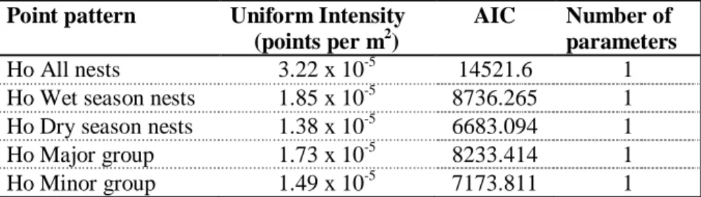
4.3.1 Models of homogeneity (stationary Poisson models). ... 26
4.3.2 Models of inhomogeneity (Non-stationary Poisson models)... 26
4.4 HIGHER-ORDER PROPERTIES OF GORILLA NEST SITE DISTRIBUTION. ... 33
4.5 SIMULATION OF THE FINAL FITTED MODELS. ... 37
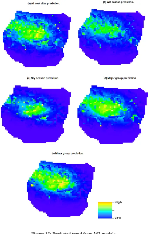
4.6 PREDICTION FROM THE FINAL M3 MODEL. ... 39
4.7 MULTI-TYPE (BIVARIATE)POINT PATTERN ANALYSIS. ... 41
4.7.1 Summary statistics. ... 41
4.7.2 Test of independence between Major and Minor group nest sites. ... 42
4.8 MULTI-TYPE MODEL FITTING (MULTI-TYPE TREND). ... 43
4.8.1 Stationary (homogeneous) multi-type Poisson models (HMPP). ... 43
4.8.2 Test for inhomogeneous Multi-type Poisson process (IMPP). ... 44
4.8.3 Modelling for inter-group interaction... 45
CHAPTER 5: DISCUSSION, RECOMMENDATIONS AND CONCLUSION. ... 48
5.1 DISCUSSION. ... 48
5.1.1 Model fitting and selection. ... 48
5.1.2 Interaction between nest sites. ... 49
5.1.3 Effect of covariates. ... 50
5.2 CONCLUDING REMARKS... 53
5.3 DIRECTIONS FOR FURTHER ANALYSIS. ... 54
REFERENCES ... 55
APPENDICES ... 58
x
APPENDIX B:QUADRAT COUNT STATISTICS FOR DIFFERENT NEST SITE PATTERNS. ... 59 APPENDIX C:INTENSITY FUNCTIONS FOR FINAL MODELS (M3MODELS)... 61 APPENDIX D:R SCRIPT WRITTEN FOR ANALYSIS. ... 62xi
INDEX OF TABLESTable 1: Point pattern categories used for analysis. ... 11
Table 2: Vegetation (habitat) categories adopted for the study. ... 12
Table 3: Constant intensity values for the various point pattern categories. ... 26
Table 4: Summary of best fit models of inhomogeneity with covariates only (M1 Models). 27 Table 5: Summary of best fit models of inhomogeneity with covariates and Cartesian coordinates (M2 Models). ... 30
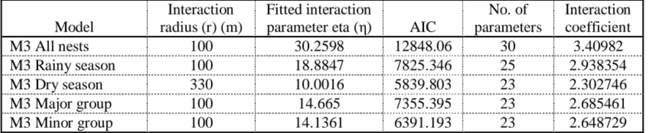
Table 6: Fitted parameters for the Area Interaction model. ... 35
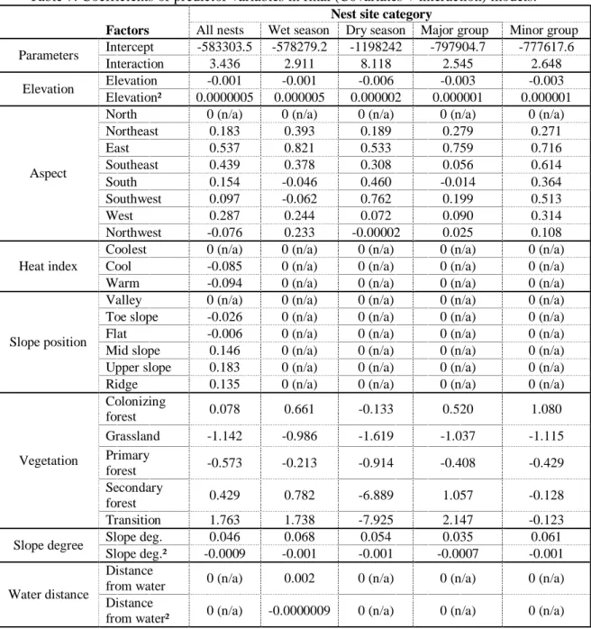
Table 7: Coefficients of predictor variables in final (Covariates + interaction) models. ... 39
Table 8: Summary statistics of the two gorilla groups nest site data. ... 42
Table 9: Constant intensity values for bivariate point patterns... 43
Table 10: Parameters of fitted Multi-type Interaction (MT) models... 46
Table 11: Ranking of categorical factor levels according to their effect on nest site distribution... 51
xii
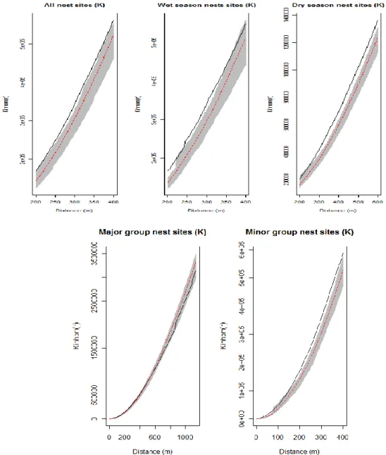
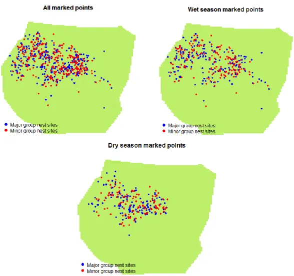
INDEX OF FIGURESFigure 1: Map of gorilla distribution (taken from Oates et al (2007)) ... 5 Figure 2: The Kagwene Gorilla Sanctuary ... 9 Figure 3: Flow chart of overall methodology implemented in analysing nests site data and fitting mode ... 13 Figure 4: Kernel-smoothed intensity for different point patterns. ... 23 Figure 5: Second-order summary K and L functions for different nest site categories. The black line indicates the empirical K function while the grey band indicates the envelope from 99 simulations. ... 25 Figure 6: Lurking variable plots for models including covariates only against continuous covariates. Solid lines represent empirical cumulative Pearson residuals for each model while dotted lines represent 5% error bands. ... 28 Figure 7: Cumulative Pearson residuals for each model against Cartesian coordinates. Solid lines represent empirical cumulative Pearson residuals for each model while dotted lines represent 5% error bands. ... 29 Figure 8: Lurking variable plots for models including covariates and Cartesian coordinates against continuous covariates. Solid lines represent empirical cumulative Pearson residuals for each model while dotted lines represent 5% error bands. ... 31 Figure 9: Generalized (Inhomogeneous) K functions with envelopes plotted from 99 simulations of the combined (M2) models. ... 32 Figure 10: Pseudo-likelihood profiles for estimating values of the irregular parameter (interaction radius) for the Area Interaction model. Green dashed line shows the r values at which pseudo-likelihood was maximized. ... 34 Figure 11: Generalized K Functions for the final trend plus interaction models. The shaded region (grey) represents envelopes from 99 simulations of each model, while the black solid line represents the empirical function from the fitted model. ... 36 Figure 12: Original nest site locations (Blue) and simulated locations (Red) from the final trend plus interaction models for the different nest site categories in the Kagwene Sanctuary. ... 38 Figure 13: Predicted trend from M3 models ... 40 Figure 14: Marked spatial point patterns of two gorilla groups nest sites in the Kagwene Sanctuary, Cameroon. ... 41
xiii
Figure 15: Second-order summary statistics for bivariate (multi-type) point pattern. The black line represents the empirical multi-type K function while the grey line indicates envelopes computed from 99 simulations of CSRI. ... 43 Figure 16: Inhomogeneous multi-type K functions for fitted multi-type models. The black lines represent the empirical inhomogeneous K functions while the grey bands represent envelopes computed from 99 simulations of the fitted models. ... 45 Figure 17: Goodness-of-fit plots for higher-order bivariate interaction models. The black lines represent the empirical inhomogeneous K functions while the grey bands represent envelopes computed from 99 simulations of the fitted models. ... 47 Figure 18: Summary plot of AIC values obtained for different models for each point pattern. Model categories on x-axis are: Ho-Models = Stationary model (univariate), M1-Models = inhomogeneous Poisson model with covariates only, M2-Models = inhomogeneous Poisson models with covariates and Cartesian coordinates, M3-Models = Combined model with covariate effect and Inter-point Interaction, and MT-Models = Multitype (bivariate) models with Inter-type interaction. ... 48 Figure 19: A view of the Kagwene Gorilla Sanctuary from above ... 491
CHAPTER 1:
INTRODUCTION
1.1 Study background.
One important requirement to the success of wildlife conservation is the
understanding of the behavior (etho-ecology) of the wildlife species especially with
reference to its environment. Obtaining an understanding of animal behavior through
field studies is important for designing captive breeding programs for endangered
species and in helping to conserve endangered wild populations. Without such
knowledge, conservation programs may result in drastic waste of resources, money
and time. For centuries, conservation scientists have sought this understanding and
continue to do so as new species of animals get discovered or as species get split into
subspecies. About a hundred years ago (1904), eight skulls of gorillas found in the
Cross River region of Nigeria and Cameroon were examined by the German
taxonomist Matschie, and this cranial examination revealed distinctions between the
Cross River Gorilla (CR gorilla) and other Western Lowland gorillas. He proposed
that this group of gorillas was distinct enough to constitute a separate gorilla species,
the Gorilla diehli (Sarmiento and Oates 1999). Other researchers disagreed with
Matschie, asserting that the CR Gorilla was actually a subspecies of the Western
Lowland gorillas, and should be known as the Gorilla gorilla diehli (as they are
known today). For some years later, gorilla surveys died down in this region and the
subspecies was thought to be lost until the 1980s when gorilla groups were
rediscovered in the Mbe Mountains (Sarmiento and Oates, 1999), and further surveys
revealed the existence of gorillas (Gorilla gorilla diehli) in different parts along the
Cross River region. Today, it appears on the International Union for Conservation of
Nature (IUCN)‟s Redlist as the most critically endangered primate (IUCN 2005).
Since the rediscovery of this subspecies, research has been geared towards
understanding their behavior for effective conservation practices. Research on gorilla
groups along the landscape reveals that they actually portray different behavioral
characteristics in different habitats (Sunderland-Groves 2008). Sunderland-Groves
actually describes them as „adaptable‟ in terms of feeding behavior because they tend
to have different diet choices in different localities. It is usually therefore necessary
to study each group of gorillas discovered, since it may be misleading applying
2
results of studies from one group to other groups. A myriad of studies have been
carried out towards understanding the ecological behavior of Western Lowland
gorillas (Brugiere and Sakom 2001; Casimir 1979; Goldsmith 2003; Mehlman and
Doran 2002; Remis 1993; Tutin et al. 1995) but very few have sought the
investigation of the behavior of CR gorillas (McFarland 2007; Sunderland-Groves
2008; Sunderland-Groves et al. 2009; De Vere et al. 2010). Most of the studies on
CR Gorillas have been based on the effect of anthropogenic activities on nesting
behavior (De Vere et al. 2010) and on seasonal distribution patterns
(Sunderland-Groves et al. 2009) using ecological assessment and classical statistical methods to
analyze nest site data. However, none of these studies has been geared towards
spatial statistical methods, or on modeling and predicting nest site distribution. We
believe that spatial point pattern analysis of nest site distribution will provide
valuable insights to the effect of environmental variables on nest site distribution, the
effect of interaction between nest site locations and on interaction between different
gorilla groups. This thesis follows this line of research by utilizing the power of
computational spatial point pattern statistical methods to mine into the nesting
behavior of the rarest ape currently known to man, the Cross River (CR) Gorilla.
1.2 Objectives of study and research questions.
The overall objective of this study is to analyze the spatial distribution of CR gorilla
nest sites in the Kagwene sanctuary of Cameroon utilizing spatial point pattern
modeling methodology. The study was intended to characterize nest site distribution
in the sanctuary, and to fit models that can estimate an intensity function for nest site
distribution.
The study set out to answer the following specific questions:
- Are gorilla nest sites randomly distributed in the sanctuary or are there any
ecological processes going on that cause them to either cluster or disperse? It was
our goal to verify if nest site distribution is uniform in the sanctuary, and
conforms to a random rather than a non-stationary process. If nest site
distribution is not random, what other pattern does it exhibit?
3
- How does each of the selected covariates affect nest site selection by CR gorillas
in the sanctuary? This study was designed to verify whether or not the selected
variables affect nest site distribution in the sanctuary and if they did, how?
- Can nest site distribution be explained solely by environmental variables or there
exists some higher-order interaction between points? If nest site distribution was
not in conformity to an inhomogeneous Poisson Process (IPP), then what is the
level of higher-order interaction that exists between nest sites?
- What is the relationship between nest sites of the Major gorilla group and those
of the Minor group in terms of spatial location? It was the aim of this study to
verify if, and to what level there was a relationship between nest site location of
the Major group and the Minor group. Do they repel or attract each other, or there
simply is no higher-order relationship between them?
1.3 Structure of the thesis
This thesis is organized into five chapters, which follow a chronological flow of
ideas as follows:
Chapter 1- Introduction.
This chapter presents a background to the study, objectives and structure of this
thesis.
Chapter 2- Gorilla distribution and conservation and application of spatial point
pattern analysis.
This chapter reviews literature related to the distribution of gorillas in general, their
conservation status and ecological behavior.
Chapter 3- Materials and Methods.
Here, we present the software tools used for the thesis, sources and description of
data and analysis methods implemented in the study.
Chapter 4- Results of analysis.
In this chapter, we present the results obtained from statistical analysis of the data.
Chapter 5- Discussion, future research and conclusion.
We present discussion on the results of analysis in this chapter. Recommendations on
the directions for future research, and general conclusions are also presented here.
4
CHAPTER 2: GORILLA CONSERVATION AND SPATIAL POINT PROCESS MODELLING.
2.1 Gorilla subspecies and conservation status.
The largest of living primates - gorillas are divided into two species: Gorilla gorilla
(Western gorilla) and Gorilla beringei (Eastern gorilla). These are further divided
into four subspecies; Gorilla gorilla gorilla (the Western lowland gorilla), Gorilla
gorilla diehli (the Cross River gorilla), Gorilla beringei graueri (the eastern lowland
or Grauer‟s gorilla) and Gorilla beringei beringei (the Mountain gorilla) (Bergl
2006). All these subspecies of gorilla are endangered (IUCN 2005) as a result of such
anthropogenic and natural factors as hunting, habitat loss, and diseases (especially
the Ebola virus) but the G. g. diehli is the most critically endangered of them all, and
of all apes put together (Mittermeier et al. 2006).
Cross River gorillas number hardly more than 300 in the wild today (Bergl 2006;
Sunderland-Groves 2008; Oates et al. 2007; Sunderland-Groves et al. 2003) and this
population is scattered over about eleven habitats in Nigeria (Afi mountains, Mbe
Mountains, Boshi Extension) and Cameroon (Takamanda South, Takamanda East,
Takamanda North, Kagwene Mountains, Bechati-Lebialem) and along the
Cameroon-Nigeria border (Okwangwo-Takamanda) (Bergl 2006).
2.2 Geographical distribution of gorillas.
All four gorilla subspecies are found exclusively in the African continent. They all
range in forest regions (Figure 1). Gorillas range in both highland and lowland
regions. In the east of Africa, the Gorilla beringei beringei is a highland subspecies
(commonly referred to as Mountain gorillas) while the Gorilla beringei graueri is a
lowland species (commonly called the Eastern lowland gorilla). To the west/central
Africa are gorillas of the species Gorilla gorilla. Of the two subspecies that make up
this group, the Gorilla gorilla gorilla is a lowland subspecies (Western lowland
gorillas) while the Gorilla gorilla diehli (Cross River Gorilla) is commonly located
in hilly and difficult terrains, sometimes measuring over 2000 m in height. Of all
four subspecies, the Cross River gorilla (the subspecies for this study) is the most
northerly and westerly in extent.
5
Figure 1: Map of gorilla distribution (taken from Oates et al (2007))
2.3 Behaviour of the Gorilla gorilla diehli.
Gorillas have been described as adaptable in terms of diet because they rely on
different food types in different regions (Sunderland-Groves 2008). Like other
gorillas, CR Gorillas spend a greater part of their day eating, but differ from other
Western gorillas in choice of diet (Oates et al. 2007) CRGs feed on herbaceous
plants throughout the year, and a variety of fruits when available. In the Kagwene
Sanctuary, they feed on a variety of fruits such as figs, Psychotria sp. and „aga‟, and
herbs, such as, Zingiberaceae (Afframomum sp), Amorphophallus difformis,
Acanthaseae, Commelinaceae (Commelina cameroonensis, Palisota mannii)
(WCS-TMLP long-term records). These food sources constitute a major habitat requirement
for the gorillas. Any activity that causes a destruction of these sources therefore is
expected to play down on the very existence of CRGs in this locality.
In the Kagwene Sanctuary, the gorillas appear to range as two social groups, the
Major (seven to nine in number) and the Minor group (five to seven in number) with
overlapping home ranges (WCS-TMLP long-terms records). Each of these social
6
groups is led by a dominant male- the silverback. These groups move about in search
of food in the day, and construct sleeping nests almost every night. In the dry season,
they construct many nests on the ground while more tree nests are constructed in the
rainy season (Sunderland-Groves et al. 2009). Each member of the group, in most
cases, sleeps in one nest so that it is possible to know the number of gorillas at each
nest site from the number of nests constructed. Exceptions are in cases where there is
a juvenile in the group, and in that case may share a nest with an adult gorilla. Nest
heights in Kagwene measure up to about 35m (Sunderland-Groves 2008). Studies on
the nesting of CRGs in Makone, Obonyi and Basho have revealed that CRGs
construct most of their nests in closed canopy forests and very few under open
canopies (Sunderland-Groves 2008). Gorillas in the Kagwene sanctuary are also
noted to construct nests on precipitous slope, which is probably attributed to security
reasons (Wiseman 2008).
2.4 Threats to gorilla conservation.
The conservation of CR gorillas is being undermined by a myriad of human factors
in different localities. Human activities carried out in and around gorilla habitats are
noted to cause habitat loss and/or modification. Such activities include crop farming,
pastoral farming, hunting, deforestation caused by bushfires or extraction of timber
and non-timber forest products and the like. These factors have been addressed by so
many researchers in different localities where CR gorillas are found (Bergl 2006;
IUCN 2005; Mittermeier et al. 2006; Neba 2008; Oates et al. 2007; Sarmiento and
Oates 1999; Sunderland-Groves 2008; Sunderland-Groves et al. 2009). Previous
studies have also explained the influence of some of these factors on gorilla behavior
and existence. However, aside from these human-induced factors, the current study
holds that it is equally important to explain the behavior of the gorillas in terms of
the physical terrain in which they find themselves. CR gorillas are often found in
very difficult-to-access terrain, which usually makes field research an unenviable
task. It is therefore worth investigating how much of a threat the natural environment
in which they find themselves can be. This was a motivation to this study and the
reason why the factors included to the models were mostly natural and not
anthropogenic.
7
2.5 Application of Spatial point process modeling.
Spatial point processes are models built for random point patterns in different
dimensional spaces (usually 2 or 3-dimensions). It is “...a stochastic process in which
we observe the locations of some events of interest within a bounded region A.”
(Bivand et al. 2007). An event here refers to actual observations of points, while the
region A is usually considered or termed the window of observation (Baddeley 2008;
Baddeley and Turner 2006). Spatial point process modeling is a major study within
the field of spatial statistics that does not only discover the distributional pattern
inherent in a point dataset, but also goes beyond to explain why observed points
follow a particular pattern.
This modeling technique is an analogy of regression models in classical (non-spatial)
statistics, and can be applied to a wide range of fields including forestry and plant
ecology (e.g. explain position of particular tree species in a forest stand),
epidemiology (e.g. how and why a particular disease is, or group of diseases are
distributed in a settlement), seismology (e.g. distrubution of earthquake epicenters),
wildlife ecology (e.g. location of nests or burrows of animals), geography (e.g. what
affect settlement location), amongst many others.
The essence of spatial point processes modeling is usually to verify whether or not
points in a point pattern are distributed in a random manner. Therefore, in point
process modeling, the first and most basic tests are based on the concept of Complete
Spatial Randomness (CSR) – where events are assumed to be randomly distributed.
Any point pattern modeling basically would end at this stage if points in the pattern
are tested to follow a random distribution. A rejection of spatial randomness in
distribution is the ground on which further models are built. If a test for CSR proves
that the points are clustered or dispersed, then we are often faced with the task of
explaining why any of these patterns might exist. Model fitting for a point pattern
that is not completely random is done with the aim of obtaining the best model that
can best explain the distribution of points in the dataset, that is the best model to
provide an intensity function for the data. Point process models are important not
only to understand the effect of different factors on point distribution, but also to
predict point occurrence for other areas where point distribution is unknown.
8
In the R statistical software, spatial point pattern models can be fitted with packages
such as spatstat (Baddeley and Turner 2005) and SPLANCS (Rowlinson and
Diggle 1993). These packages provide extensive functionality for model fitting,
simulation and prediction, but it is worth noting that they are still limited in the
functions built in and in the volume of data they can handle (the latter is a general R
limitation). Before models can be fitted using these packages, other support packages
are needed for data preparation and input into R. Together with these complementary
packages, spatstat and SPLANCS provide an amazingly powerful environment
for point pattern modeling.
9
CHAPTER 3: MATERIALS AND METHODS.
This chapter describes the methodology implemented in analyzing gorilla nest site
data and modeling. It presents the study area, sources of data and tools used to
analyze the data.
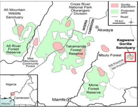
3.1 The study area.
The Kagwene Gorilla Sanctuary (06º05‟-06º08‟N: 09º42-09º48‟E, KGS, Figure 2) is
located along the North West-South West Regional boundary of Cameroon and
covers an area of 19.44 km². It is one of over 11 habitats where CR gorilla
populations are said to exist. The Kagwene Mountains are of the Western Highlands
of Cameroon, and form part of a chain of mountains from Bioko to Plateau State,
Nigeria, with altitudes measuring over 2000m a.s.l.
Figure 2: The Kagwene Gorilla Sanctuary
(Sunderland-Groves et al. 2009).
Climate is marked by a rainy season (April to October), and a dry season (November
to March). Average annual rainfall is about 3,774mm; with mean temperatures
ranging between 14.6˚C and 22.3˚C (Kagwene Research Camp long-term records,
2003-2008). The KGS has a dense drainage network, constituting a watershed that
supplies all the communities around it. Vegetation is composed of grassland and
10
galleries of montane forest. The area supports a variety of plant and animal species.
It is a protected area, and home of the critically endangered Cross River gorilla
(Gorilla gorilla diehli). The Wildlife Conservation Society (WCS) Takamanda-Mone
Landscape Project (TMLP) runs a research camp in the sanctuary, and has collected
and filed gorilla nest site data since 2003. The gorilla population in the KGS is
genetically distinct from other CR Gorilla groups, but although they seem to be
isolated from gorillas of other localities, genetic analyses still reveal some migration
to other neighbouring populations still occur (Bergl 2006; Bergl and Vigilant 2007).
Daily gorilla tracking reveals that the gorillas range in two bands of six (called Minor
(M) group) and eight (called Major (J) group). The sanctuary is surrounded by nine
rural settlements.
3.2 Materials 3.2.1 Analysis tools.
The primary tool used for data analysis was the R statistical software version
2.12.1 (R Development Core Team 2009). Several packages within the R
environment were used for reading data and performing analysis, but the principal
package for implementation and statistical analysis was spatstat. Nest site data
were collated and formatted using Microsoft Office Excel. ArcGIS was used for
preliminary visualization of data layers, and preparation of covariates. The covariates
were exported from ArcGIS environment as American Standard Code for
Information Interchange (ascii) files and read into R. Microsoft Office was used for
final reporting of results.
3.2.2 Gorilla nest site data.
We utilized 640 nest site locations recorded in the Kagwene Groilla Sanctuary
collected between 2006 and 2009 for the analysis. These locations were generously
provided by the Wildlife Conservation Society Takamanda-Mone Landscape Project
(WCS-TMLP) Cameroon. These data are collected during daily gorilla tracking in
the sanctuary. The researchers go out each day, follow the gorilla trails until they get
to the site where the gorillas built their nests. The number of nests per site differs
(usually more than one), but only one GPS record (point) is taken at each site. It is
therefore necessary to emphasize that this analysis is based on NEST SITE locations
and not NEST locations.
11
The gorillas in the KGS are known to range in two bands (groups) called the Major
(J) group and the Minor (M) group. For the purpose of this analysis, we classified
nest sites with less than or equal to 6 nests as Minor group and sites with more than 6
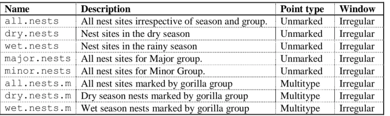
nests as Major. Data were split into various categories and properties extracted for
each category. Point pattern categories analyzed during this project were as follows
(Table 1):
Table 1: Point pattern categories used for analysis.
Name Description Point type Window
all.nests All nest sites irrespective of season and group. Unmarked Irregular
dry.nests Nest sites in the dry season Unmarked Irregular
wet.nests Nest sites in the rainy season Unmarked Irregular
major.nests All nest sites for Major group. Unmarked Irregular
minor.nests All nest sites for Minor Group. Unmarked Irregular
all.nests.m All nest sites marked by gorilla group Multitype Irregular dry.nests.m Dry season nests marked by gorilla group Multitype Irregular wet.nests.m Wet season nests marked by gorilla group Multitype Irregular
Our interest was to verify the properties and model the distribution of all gorilla nests for all years, for each season and for each gorilla group. All nest site locations from April to October were classified as wet season and nest locations from November to March were classified as dry season nests.
3.2.3 Covariates (Predictor variables).
Seven environmental covariates or explanatory variables were used for the study. The focus was to verify how these covariates explain nest site location by the gorillas. It was intended that these covariates would reflect the natural environment as much as possible, although there was an exception of disturbed forest. The covariates were as follows:
a. Elevation: This was the digital elevation of the study area derived from a 30m digital elevation model (DEM) obtained from ASTER (freely available for the whole world – Aster GDEM). Values were in meters.
b. Heat Load Index (Beer’s Aspect): Calculated from the DEM using the ArcToolbox “Topography”. This characterizes the landscape into the potential heat that will be incident at any point on the terrain. It implements the formula:
Heat Load=1+cos ((45º-aspect)/slope degree).
The index ranges from 0-2, and is set to maximum for NE slopes which is the coolest slope. We reclassified the indices derived into:
12
- 0 to 0.999 = South slopes --- Warmest.- 1 to 1.999 = NW/SE slopes --- Cool. - 2 = NE Slopes --- Coolest.
c. Aspect: This was calculated from the DEM using the surface analysis provided by the ArcGIS Spatial Analyst tool.
d. Slope degree: This was calculated from the DEM using the surface analysis provided by the ArcGIS Spatial Analyst tool.
e. Slope position: Calculated from the DEM using the ArcToolbox “Topography”. It classifies the slope into six landform categories (Valley, Toe Slope, Flat, Mid slope, Upper slope and Ridge).
f. Distance from water channel: This was a measure of the Euclidean distance away from a water channel, expressed in meters.
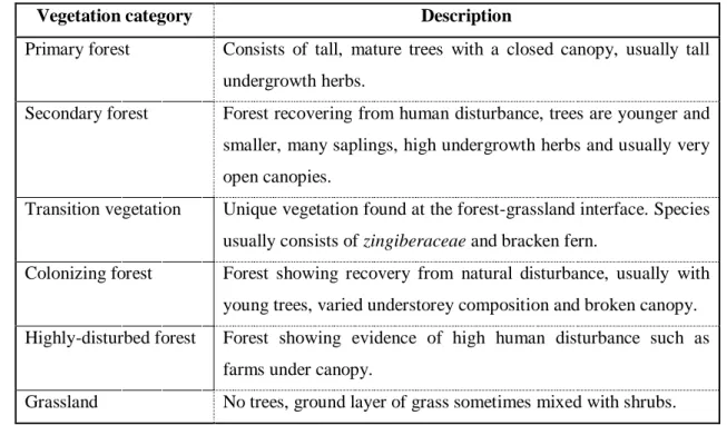
g. Vegetation type: This was a broad classification of vegetation into 6 categories as shown
on Table 2.
Table 2: Vegetation (habitat) categories adopted for the study.
Vegetation category Description
Primary forest Consists of tall, mature trees with a closed canopy, usually tall undergrowth herbs.
Secondary forest Forest recovering from human disturbance, trees are younger and smaller, many saplings, high undergrowth herbs and usually very open canopies.
Transition vegetation Unique vegetation found at the forest-grassland interface. Species usually consists of zingiberaceae and bracken fern.
Colonizing forest Forest showing recovery from natural disturbance, usually with young trees, varied understorey composition and broken canopy. Highly-disturbed forest Forest showing evidence of high human disturbance such as
farms under canopy.
Grassland No trees, ground layer of grass sometimes mixed with shrubs. Sources: (Neba 2008; Sunderland et al. 2003; Wiseman 2008)
3.3 Methods.
13
Figure 3: Flow chart of overall methodology implemented in analysing nests site data and14
3.3.1 Characterization of gorilla nest site distribution.
First-order characteristics.
First-order characteristics are characteristics related to variations in the mean value of the spatial process. They are a measure of the distribution of events in the study area (Bivand et
al. 2007; Diggle 2003; Møller and Waagepetersen 2003). First-order characteristics do not
provide any information on interaction between events in the point pattern, but yield a general idea about their spatial distribution; that is they only provide information on the global spatial trend of point distribution. This characteristic was provided by estimation of the kernel-smoothed intensity of the different point pattern categories. That is, given each point pattern, the kernel-smoothed intensity was used to estimate the general location of events. The Kernel-smoothed intensity is represented by a function λ(u), which measures the mean number of events per unit area at the point u. Therefore for a general location s and a given dataset X, the kernel-smoothed intensity is given by
n i i ib b bK
s
x
s
C
s
1)
(
)
(
1
)
(
Equation 1: Kernel-smoothed intensity estimation.
where Kb( ) is a kernel with band b > 0, and Cb( ) is an edge correction factor (Diggle 2003; Yang et al. 2007).
Testing for Complete Spatial Randomness.
a. Second-order characteristics of nest site distribution.
Besides first-order properties, second-order characteristics provide information on event interaction in a point pattern. Second-order properties are thought to offer the best way to present, statistically, the distributional information inherent in point patterns and in explaining the correlation between them (Illian et al. 2008). Because they consider the relationship between points at different distances, second-order properties are credited for being able to estimate the distributional correlation between points at long range, far beyond the nearest neighbors only. In this study, Ripley‟s K function and Besag‟s L function (a transformation of the K function) were used to obtain the second-order characteristics and test for Complete Spatial Randomness of gorilla nest site distribution.
The main idea behind the K function (Ripley 1977) is the consideration of the average number of points found within a distance r from a typical point. If λK(r) denotes the mean number of points in a disc of radius r centered around a typical point xi, and n denotes the
15
number of points found in a window W, and ni(r) = N(b(xi, r)\{xi}) is the number of points of N that occur within a distance r from the typical point xi, then excluding xi itself,
n i ir
n
n
r
1)
(
1
)
(
Equation 2: estimate of the K function estimates λK(r). Therefore,
number
E
r
K
(
)
(
of events within a distance r of an arbitrary event)where E( ) is the expectation operator and λ is the intensity or the mean number of points per unit area.
The L function is a transformed (variant) form of Ripley‟s K function. It is defined as
) ( ) (r K r L Equation 3: The L function
Clearly, it yields the same information as the K function, but is assumed to have some advantages in that when testing for Complete Spatial Randomness, it is easier to visualize the graph of the L function than its K counterpart. It is also known that for increasing distances
(r), there is increasing fluctuation in the estimated K function, a fluctuation that is stabilized
by the root transformation provided by the L function (Illian et al. 2008).
The observed behavior of K(r) and its transformation, L(r) with respect to πr² is expected to yield information on the nature of interaction between points in a point pattern. Where
K(r)>πr² or L(r)>πr², it indicates a clustered point process where the typical point xi has some very near neighbors and the local point density around xi is larger than the number of points per unit area (λ) in the point process. K(r)<πr² or L(r)<πr² indicates that the typical point xi is isolated and the local point density around it is smaller than λ; while K(r)=πr² or L(r)=πr² indicates a random process. Larger differences between K(r) and πr² (and therefore
between L(r)<πr²) indicate greater clustering or regularity in point distribution, as the case may be.
The computed K function and L function were not only compared to the theoretical functions under CSR, but also the upper and lower bounds of envelopes simulated independently under CSR, but having the same intensity as the test data. Envelopes are also used together with the
16
distance-based functions such as the K and L functions to test for goodness-of-fit of fitted models (Baddeley 2008; Baddeley and Turner 2000; Bivand et al. 2007).This study used 99 simulations of CSR to compute envelopes. Ninety-nine simulations are recommended for point process modeling and considered conventional and analogous to alpha level (α) = 0.01 in classical statistics (and 19 simulations would be analogous to α =
0.05) (Illian et al. 2008). Deviations of the computed functions from the theoretical functions
would suggest clustering (contagion) or regularity (inhibition) in nest site distribution, where, as mentioned before, K(r) > πr² and L(r) > πr² suggest clustering and K(r) < πr and
L(r) < πr² suggest regularity. In spatstat, the K function, L function and envelopes are
computed by built-in functions Kest, Lest and envelope respectively.
The reasons for testing for CSR were generally 3-fold: (1) A rejection of CSR is a prerequisite for any further modelling of an observed point pattern, (2) testing for CSR helps us explore a data set and formulate alternative hypothesis and (3) CSR serves as a dividing hypothesis between clustering and regularity. Under CSR, there is equal probability for all events occurring at any position in the study region; and the position of each event does not in any way affect the position of any other event (events are independent).
b. Quadrat-counting test of CSR.
Quadrat counting tests were also used to test for the hypothesis of Complete Spatial
Randomness (CSR). Quadrats were determined by different levels of covariates. The quadrat test utilizes a chi square (χ²) test of hypothesis to verify whether or not for different levels of covariates, observed nest site frequency differed significantly from expected frequency. The tests were carried out at α = 0.05. In spatstat, the quadrat test is provided by the formula quadrat.test.
3.3.2 Model fitting to data.
Models were fitted to estimate an intensity function that could best describe each of the point patterns.
1. Homogeneous Poisson Process (HPP).
These are the null (stationary) models that assume a uniform distribution of points within the study area (W). They can also be described as isotropic (Bivand et al. 2007) where the occurrence of an event does not affect the occurrence of another within the study area. Intensity (λ) is constant in W, and the second-order properties only depend on the relative positions of two points (Bivand et al. 2007). HPP can be formally described as having the following characteristics:
17
a. The number of events in a region W, with area |W| is a Poisson distribution with meanintensity λ|W|, where λ is the constant intensity of the point process.
b. The number of events n occurring in an area W area uniformly distributed in W. (Baddeley 2008; Bivand et al. 2007).
Null models were therefore fitted for each point pattern with the assumption that spatial trend was neither influenced by any covariate nor point coordinates.
2. Modeling for an Inhomogeneous Poisson Process (IPP).
In case CSR was out-ruled, it was assumed (tentatively!) that nest site locations were independent, that is, their distribution (or location probability) depended on heterogeneity of selected environmental variables and/or Cartesian coordinates of their locations and not on interaction between them (that is the assumption of an IPP). All possible combinations of environmental covariates were considered as candidate models (using the R package combinat to generate all possible combinations), and a Maximum Pseudolikelihood Estimation (MPLE) method was used to estimate coefficients for each candidate model. This method has been described as efficient, sufficient and consistent (Illian et al. 2008). MPLE is simply an approximation of maximum likelihood estimation (MLE) and is recommended for point process modeling because for many spatial point process models, the likelihood is intractable. The R package spatstat implements the MPLE using the Berman-Turner computational algorithm (Baddeley and Turner 2000; Berman and Turner 1992). It fits point process models to point data in terms of their Papangelou conditional intensity, loosely defined as the probability of an event occurring at point u given that the rest of the process coincides with the point pattern X (Baddeley and Turner 2000). Intensity is estimated as:
)
(
)
,
(
u
x
u
Equation 4: Conditional intensity function.
where β(u) depends on the spatial locations of u, and therefore stands for “spatial trend”, or environmental covariates. That is, the term β(u) can be a function of the Cartesian coordinates of u or of an observed covariate at location u, or of a mixture of both (Baddeley 2008). We first considered combinations of covariates alone, and if model diagnostics proved that the fitted models were still inadequate to explain the spatial trend, it showed that these covariates were not enough to explain nest site distribution in the sanctuary, and that there was still a spatial trend inherent in the data that was not captured by the model. In this case, Cartesian coordinates of the nest sites were introduced as a covariate to substitute for other factors that might have an effect on intensity but were not available for the analysis (such as temperature, rainfall, other human factors etc), and to enable the model capture any spatial trend caused by such factors in nest site distribution (Baddeley 2008; Yang et al.
18
2007; Rathbun et al. 2007). By implication therefore, it was assumed here that spatial trend of nest site distribution in the sanctuary was influenced by environmental covariates and other factors not considered in the model. Inhomogeneous spatial trend was modelled with intensity that is log-quadratic in continuous covariates (elevation, water distance and slope) and Cartesian coordinates. Polynomials of up to the order two were considered (as long as it converged with the MPLE) (Baddeley and Turner 2000; Yang et al. 2007). The log-quadratic intensity function in Cartesian coordinates and continuous covariates was estimated as:2 2 1 0 ( ) ( ) ) , ( log
u x
B u
B u or equivalently,)
)
(
)
(
exp(
)
,
(
u
x
0
1B
u
2B
u
2
Equation 5: Conditional intensity function as a log-quadratic of continuous variables. where θ1, θ2…θn estimated parameters, and B(u) represents spatial trend or covariate. The log-quadratic intensity function is fitted through the formula polynom formula in spatstat.
3.3.3 Model selection.
The different possible combinations of environmental covariates for modeling gave a total of 127 competing candidate models for each nest site point pattern category. From these, the model that could best describe the observed pattern of nest site distribution had to be chosen. The Akaike‟s Information Criterion (AIC) was used for this purpose (Akaike 1973). It is defined as:
k
likelihood
AIC
2
max(log
)
2
Equation 6:Akaike‟s Information Criterion.
where k is the number of parameters in the model. The AIC is a handy method of selecting the best of competing models over goodness-of-fit because it minimizes the effect of model complexity (increased number of parameters) in selecting the better model.
3.3.4 Model diagnostics and verification of assumption of inhomogeneity.
Residual analysis was used to validate the best fit models for each nest site category. Lurking variable plots were computed for each model, plotting the cumulative Pearson residuals of the model against each of the continuous covariates (elevation, distance from water channel and slope percent) and Cartesian coordinates. If the model were a good fit, then the cumulative Pearson residuals should approximate to zero (an analogy to the fact that residuals for a regression model always sum up to zero in classical statistics such as GLM) and when plotted for each continuous variable should fall within the error bands (2
bands).19
The goodness-of-fit of models was also tested by computing envelopes from simulations of the fitted models and observing the behaviour of the computed K function. We utilized thegeneralized (inhomogeneous) version of Ripley‟s K function (Baddeley et al. 2000) and 99
simulations to test for goodness-of-fit of the models (Baddeley and Turner 2000). Ripley‟s K
function is defined only for stationary (homogeneous) point processes, but for non-stationary
process, it is necessary to utilize a function that accounts for inhomogeneity. The generalized (or inhomogeneous) K function therefore is, as the name implies, a generalisation of Ripley‟s
K function to suite inhomogeneous processes (Baddeley 2008). These are implemented in
spatstat through the functions envelope and Kinhom.
3.3.5 Modelling for inter-point interaction (Higher-order properties).
In all the models fitted before (including covariate and Cartesian coordinate effect), diagnostics (both residual plots and inhomogeneous K functions) still showed that the models were inadequate to explain the spatial trend in nest site distribution, and that the assumption of an IPP was not adequate. This therefore was a motivation for fitting higher-order models for the data. The aim of this was to verify interaction between points. It was assumed that the spatial distribution of nest sites could be explained by spatial covariates and as well as interaction between nest site locations. An interaction parameter could therefore be added to the fitted intensity function, in which case the function will take the form:
)
,
(
)
(
)
(
)
,
(
log
u
x
0
1B
u
2B
u
2
3C
u
x
or equivalently,
(u,x)exp(
0
1B(u)
2B(u)2
3C(u,x)) Equation 7: Conditional Intensity including interaction parameter.where θ1, θ2…θn are estimated parameters, B(u) represents spatial covariates or Cartesian coordinates and C(u, x) represents the inter-point interaction term.
The Area Interaction model was chosen amongst different options such as the Strauss process (Strauss 1975) and the Geyer saturation process (Geyer 1999) to fit models portraying higher-order properties of gorilla nest site distribution. It was chosen over the Strauss process because, although the model was originally meant to describe clustering between points in a point process and is credited for being a prototype to cluster models, further research (Kelly and Ripley 1976; Turner 2009) has demonstrated that mathematically, it is not an adequate process to model interaction because the density of such a process for a point pattern X={x1, x2, … xn) is not integrable, unless n is fixed. It has also been argued that unlike the Strauss process, the Area-Interaction process is not based on
20
a simple pair-wise interaction but on a much more complex structure of interactions (Baddeley 2008; Illian et al. 2008). The Area Interaction model was also chosen above the Geyer‟s saturation process simply because it portrayed less computation time in R.The area-interaction process with a disc of radius r is defined as a point pattern process with probability density given by:
) ( ) ( ) ,..., (xi xn kn x Ax f
Equation 8.: Probability density function of an Area-Interaction process.
where xi,…,xn are the points in the point pattern, k is the intensity parameter,
η
is the interaction parameter and A(x) is the area of the region created by the union of discs or radiusr centred at the points xi,…,xn and α represents a normalizing constant (Baddeley and Van Lieshout 1995).
In spatstat, the Area-Interaction process is implemented by the function AreaInter. In this process, the aim was to obtain the interaction parameter eta (η). Values of η < 1 suggest an „ordered‟ or „inhibitive‟ pattern; if η > 1, then the model describes a clustered or attractive pattern. If η = 1, then there is no interaction between points, and the pattern corresponds to a Poisson process. If η = 0, then a hardcore process is encountered in which there are no points within the hardcore distance (r) of any point in the point process; that is, there is total inhibition (Baddeley and Lieshout 1995; Turner 2009).
Estimation of the interaction radius (r) (“nuisance or irregular parameter”).
In fitting Area Interaction models, it is very important to determine an adequate value for the irregular parameter – the interaction radius. This parameter has been described as a „nuisance‟ parameter because it is usually not clear how it is derived statistically. In fact, in the R package spatstat, the model function ppm does not provide a direct estimation of this parameter. It has to be determined by some other method. It is an intricate part of the model fitting process because wrong values of the interaction parameter can cause an overestimation or underestimation of the model. (Baddeley and Turner 2000) propose that this parameter can be obtained by maximizing the profile log pseudo-likelihood for the dataset. We tried interaction radii for each dataset between 100 and 1150 by 115 steps for profile maximization. The upper bounds (1150) were chosen based on the inhomogeneous K functions (Kinhom) of each point data set. This was the maximum distance obtained from the inhomogeneous distance function. For each dataset therefore 10 interaction models were fitted and in each case, the maximum log pseudo-likelihood for each point pattern was
21
obtained. In R, the function profilepl built into the spatstat package fits the models for estimation of this parameter.3.3.6 Simulating the fitted models.
The final selected models for each point pattern included covariates, Cartesian coordinates and inter-point interaction. Simulations were made of these final models, and if the model were good enough, then the simulated points would be very similar to the original points when displayed on plots. Simulations were done using the Metropolis-Hastings algorithm (Chib and Greenberg 1995), implemented in spatstat by the function rmh.
3.3.7 Predictions from the fitted models.
The final fitted models were used to make predictions on gorilla nest site location; that is, using the final fitted models, we evaluated the spatial trend at new locations. It would be important to verify where else gorilla nest sites would occur, given the fitted model, thereby using known gorilla locations and information generated from the model (covariate effect and inter-point interaction) to obtain information about unknown nest site locations. This is provided by the function predict.ppm in spatstat (Baddeley and Turner 2000).
3.3.8 Modelling for Inter-type interaction (Multi-type Point Pattern analysis).
Previous analysis and models ignored the fact that gorillas in the sanctuary range in two groups (bands). However, there was need to consider this and model nest site distribution in terms of interaction between the two groups of gorillas – the Major group and the Minor group. We therefore created bivariate point patterns in which each nest site location was given an additional attribute – the gorilla group to which it belonged. This is a Multi-type (bivariate) Point Pattern.
We sought to answer the following question: Are Major group nest sites clustered around Minor group nest sites or are they farther apart, OR is the pattern of occurrence of one type of event related to the occurrence of the other OR does the distribution of Major group nest sites explain the distribution of Minor group nest sites OR is there evidence that the Major and Minor group nest sites occur independently? To answer this question, we used analogues of the K and L distance functions described for simple point patterns in the preceding sections. The null hypothesis here was: There is no inter-group interaction, ie γmajor, minor = 1. If Major group nests occur independently or Minor group nests, then Kmajor, minor (r) = πr² and Lmajor, minor(r)=πr². Under repulsion, Kmajor,minor (r)<πr² (Lmajor, minor(r)<πr²) and under attraction, Kmajor, minor(r)>πr² (Lmajor, minor(r)>πr²). In spatstat, these estimations are provided by the summary functions Kcross and Lcross for Kmajor,minor and Lmajor,minor respectively. They are used to test for Complete Spatial Randomness and
22
Independence (CSRI) for a marked point pattern and they incorporate both characteristics ofrandom labelling (given the point locations X, marks are conditionally independent and
identically distributed (iid)) and independence of components (ie the sub-processes Xm of points of each mark m, are independent point processes) (Baddeley 2008; Baddeley and Turner 2000).
To fit models to the multi-type point patterns, we used the best fit models chosen for point pattern analysis (described in the preceding sections) and included marks as a factor. Inhomogeneous multi-type Poisson process models assumed that nest sites of each type (Major or Minor group) portrayed a different, non-constant intensity. Intensity was therefore modelled as a log-quadratic function of Cartesian coordinates of nest sites and environmental covariates, multiplied by a constant factor depending on the mark (Baddeley 2008; Baddeley and Turner 2006). Inhomogeneous multi-type models were therefore fitted where intensity function λ(x,y,m) at location (x,y) and marks (m) satisfies
u m y x
m
m
(( , , )) logEquation 9: Conditional intensity for multi-type point process.
where αm and βm are model parameters and u represents the value of spatial covariates, xy location of nest site or a mixture of both. Final selected models were also tested for goodness-of-fit using the K function for bivariate point patterns, implemented by Kcross.inhom in spatstat. It counts the expected number of points of type major within a given distance of a point of type minor taking into consideration varying intensities of the different types. In cases where the inhomogeneous functions still showed that the models were inadequate, we went ahead to model for higher-order properties where inter-type interaction was considered. Here, quite unfortunately, the only model currently implemented in R for fitting higher-order interaction for marked point patterns is the Strauss model. We therefore computed the models, but bearing in mind that the resulting coefficients and simulations might not be the best for the data, given the weaknesses of the Strauss process pointed out in preceding sections of this chapter (section 3.3.5).
From the fitted coefficients, the inter-type interaction coefficients were obtained for each point pattern, and intensity functions including inter-type interaction were obtained. Other procedures such as simulating the resulting models and predictions from the fitted models were as described for the univariate spatial point processes above.
23
CHAPTER 4: RESULTS OF ANALYSIS.
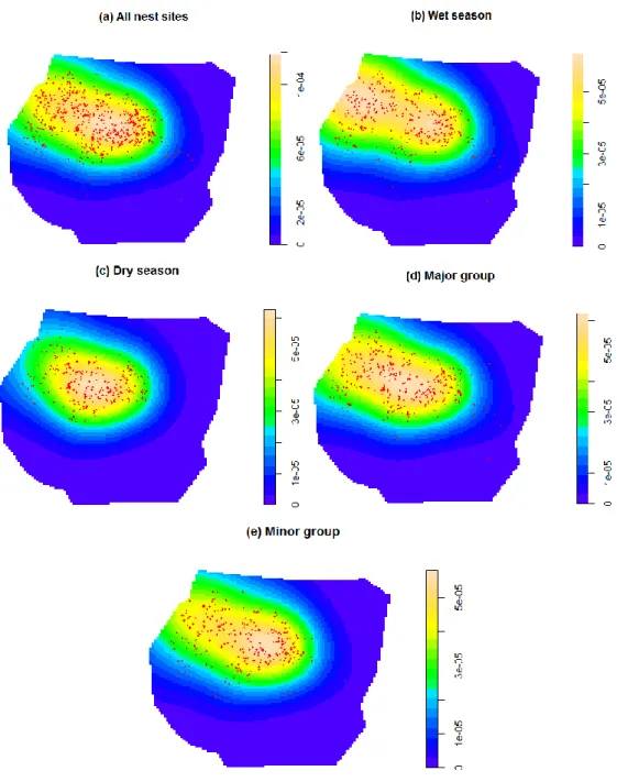
4.1 First-order characteristics of gorilla nest site distribution in the sanctuary.
A plot of the kernel-smoothed intensity for all nest site data revealed a "hot-spot" at the central extending to the northwestern part of the sanctuary, and a "cold-spot" towards the southeastern (Figure 4). These suggest that the point pattern is not completely random and is far from homogeneous, but follows another point process.
Figure 4: Kernel-smoothed intensity for different point patterns.
The results revealed by the kernel smoothed intensities suggest that the point patterns for all nests, wet season nests and dry season nests, and nests for both major and minor groups
24
follow a spatial trend that is different from uniform or stationary. That is, they suggest that nest site distribution is not isotropic in the plane. However these are only suggestive and more empirical formulations need to be carried out before we can totally out-rule complete spatial randomness.4.2 Testing for Complete Spatial Randomness in nest site distribution.
As mentioned before, the main reason for verifying second-order characteristics of nest site distribution was to test for CSR. The null hypothesis was that nest site distribution conforms to CSR or is a realization of CSR. The alternative was that nest site distribution is not a realization of CSR, but of another unspecified point process that is not completely random. Chi square statistics obtained from quadrat-count test for different nest site categories revealed significant difference in nest site distribution, given different levels of elevation, aspect, vegetation type, percent slope and distance from water body (Appendix A). This suggested that nest site distribution in the sanctuary is not completely random.
The figures below show envelopes computed from 99 simulations of the null hypothesis (Figure 5), used to further test for CSR.