Implementaion of Regional Burnt Area Algorithms for the GBA2000 initiative

(1)

Implementation of Regional Burnt Area Algorithms

for the GBA2000 Initiative

Kevin J. Tansey

with contributions from

E. Binaghi, L. Boschetti, P.A. Brivio, A. Cabral, D. Ershov, S. Flasse, R. Fraser, I. Gallo, D. Graetz, J-M. Grégoire, M. Maggi, P. Peduzzi, J.M. Pereira, A. Sà, J. Silva, A. Sousa, D. Stroppiana, M.J.P. Vasconcelos

(2)

LEGAL NOTICE

Neither the European Commission nor any person acting on behalf of the Commission is responsible for the use which

might be made of the following information.

A great deal of additional information on the European Union is available on the Internet. It can be accessed

through the Europa server (http://europa.eu.int)

EUR 20532 EN

Reproduction is authorized provided the source is acknowledged

(3)

Implementation of Regional Burnt Area Algorithms

for the GBA2000 Initiative

Kevin J. Tansey

1

with contributions from

E. Binaghi2, L. Boschetti1, P.A. Brivio3, A. Cabral4, D. Ershov5, S. Flasse6, R. Fraser7, I. Gallo2, D. Graetz8, J-M. Grégoire1, M. Maggi1, P. Peduzzi9, J.M. Pereira4, A. Sà10, J. Silva10, A. Sousa11, D. Stroppiana1, M.J.P. Vasconcelos4

1_{Global Vegetation Monitoring Unit, Joint Research Centre, Ispra, Italy} 2_{Università Degli Studi Dell’Insubria, Varese, Italy}

3_{Institute for Electromagnetic Sensing of the Environment, Milan, Italy} 4_{Tropical Research Institute, Lisbon, Portugal}

5_{International Forest Institute, Moscow, Fed. of Russia} 6_{Flasse Consulting, Maidstone, United Kingdom} 7_{Canada Centre for Remote Sensing, Ottawa, Canada} 8_{CSIRO Earth Observation Centre, Canberra, Australia} 9_{UNEP Early Warning Unit, Geneva, Switzerland} 10_{Instituto Superior de Agronomia, Lisbon, Portugal} 11_{Universidade de Évora, Évora, Portugal}

(4)

(5)

Executive Summary

As part of the Fifth Framework Programme 1999-2002 for Research,

Technological Development and Demonstration carried out by the

Joint Research Centre (JRC), the Global Vegetation Monitoring (GVM) Unit was given the task of implementing a project entitled Global Environment Information System (GEIS). One objective of the project is to provide information on disturbances to the world's vegetation cover. This involves analysis of global Earth Observation (EO) data for inventory of vegetation fires and for mapping of areas burnt. It is in this context that the GVM unit has proposed the Global Burnt Area 2000 (GBA2000) initiative.

The European VEGETATION programme partners have made a satellite image archive available as part of their VEGETATION data for Global Assessment initiative, VEGA 2000, with a financial support of CNES, JRC and VITO as a contribution to the objectives of the Millennium Ecosystem Assessment. It covers the period November 1999 to December 2000. The VEGA 2000 dataset was made available to the whole scientific community through an invitation to submit proposals. Data delivery to JRC from the VEGETATION central processing facility operated by VITO in Belgium was completed by March 2001. JRC then organized data extraction and transfer for the GBA2000 partners.

This report provides detailed information and instructions on technical and computational aspects of GBA2000. In this report, the methods adopted to process the global, daily dataset of SPOT Vegetation S1 images for the year 2000 are presented. The report is divided into sections so that the user can easily comprehend and, if necessary, repeat any of the burnt area algorithms described in this report. Following the main report, annexes provide the text of all of the

(9)

programs and tools developed by the author (with colleagues). This report does not present any analysis, assessment or interpretation of the final results. The reader is referred to non-technical reports that accompany this report for this information.

In the first chapter, characteristics of the data are presented and an overview of the approach taken to process the data is given. Chapter two describes the module written to extract data from the data archive for a particular region of interest and time period. Chapter three describes the pre-processing module. Chapter four describes the image compositing module and criteria. Chapters five to twelve describe the technical aspects of implementing operationally the burnt area algorithms developed by the GBA2000 project partners. Chapter thirteen describes the methods used to derive the final global burnt area product. A Technical Annex (provided on a CD-ROM enclosed with this report) contains detailed descriptions of all the programs used. These programs are free software; you can redistribute them and/or modify them under the terms of the GNU General Public License (GNU GPL) as published by the Free Software Foundation, under version 2 of the License. The GNU GPL is given in the Technical Annex document.

(10)

Acronyms

AML ARC Macro Language

ATSR Along Track Scanning Radiometer

BA Burnt Area

BSQ Band Sequential (Data Format)

BRDF Bidirectional Reflectance Distribution Function CART Classification and Regression Trees

CCRS Canadian Centre for Remote Sensing CNES Centre National d’Etude Spatiale (France)

CNR-IREA Consiglio Nazional delle Ricerche-Istituto per il Rilevamento Elettromagnetico dell’Ambiente (Italy) CSIRO-EOC Commonwealth Scientific and Industrial Research Organization-Earth Observation Centre (Australia)

DEM Digital Elevation Model

DN Digital Number

ENVI The Environment for Visualising Images (Image Processing Software)

FDV First Discriminant Variable

GBA2000 Global Burnt Area 2000

GIS Geographical Information System

GVM Global Vegetation Monitoring Unit (JRC, European Commission)

HDF Hierarchical Data Format

IDL Interactive Data Language

IFI International Forest Institute (Russia)

IGBP-DIS International Geosphere Biosphere Programme - Data Information System JRC Joint Research Centre (European Commission)

MEA Millennium Ecosystem Assessment

MIR Middle Infrared

MLP Multi-Layer Perceptron (Neural Network) NDVI Normalized Difference Vegetation Index

NDWI Normalized Difference Water Index

NIR Near-Infrared

NRI Natural Resource Institute (UK)

PBA Potential Burnt Area

SAA Sun Azimuth Angle

SMAC Simplified Method for Atmospheric Corrections SPOT Système Pour l’Observation de la Terre

SZA Sun Zenith Angle

SUN OS SUN Workstation Operating System

SWIR Short-wave Infrared

SWVI Short-wave Vegetation Index

TM Thematic Mapper

TREES Tropical Ecosystem Environment observation by Satellite (JRC)

UMD University of Maryland

UTL Universidade Técnica di Lisboa

VAA Viewing Azimuth Angle

(11)

1 An overview of data characteristics and image processing

This chapter serves to provide a general overview of the hardware, software and methods utilised in undertaking the processing of SPOT Vegetation S1 images to derive the GBA2000 product. The first section of this chapter discusses the characteristics of the SPOT Vegetation S1 data that will need to be processed, the format of the data and related geographical information. The second section introduces global land cover datasets, how this data was used for the project and how this data was registered with the image data. The third section introduces the main processing modules that were developed. The fourth section introduces the computational methods and systems (hardware and software) used to process the data. The fith section explains how digital elevation models (DEMs) were utilised in the project.

1.1 SPOT Vegetation global S1 data characteristics

Daily, global SPOT Vegetation S1 products for the time period, 1st December 1999 to the 31st December 2000 were stored on a large capacity disk interchange system located physically within the GVM unit of the JRC. For general information on the SPOT Vegetation platform and sensor, please refer to a wealth of literature available in remote sensing journals and on the Internet (see for example, http://www.spot-vegetation.com, http://vegetation.cnes.fr or http://www.spotimage.fr). The rationale behind using the SPOT Vegetation sensor to detect and map burnt areas is not discussed in this technical report (this is covered fully in the individual publications of the GBA2000 partners and referenced in this report). However to remind us, the four spectral bands on the SPOT Vegetation S1 sensor are as follows (also shown are their file naming convention or reference name):

• Band B0 (wavelengths between 0.43 – 0.47 µm in the blue component of the electromagnetic spectrum).

• Band B2 (wavelengths between 0.61 – 0.68 µm in the red component of the electromagnetic spectrum).

• Band B3 (wavelengths between 0.78 – 0.89 µm in the near-infrared (NIR) component of the electromagnetic spectrum).

• Band MIR (wavelengths between 1.58 – 1.75 µm in the short-wave infrared/middle-infrared (SWIR/MIR) component of the electromagnetic spectrum).

(12)

provides an estimate of the ground surface reflectance in each of the four spectral bands. This S product has been derived from the P product after being subject to an atmospheric correction using the SMAC procedure (Rahman and Dedieu, 1994). The geometric viewing conditions for each pixel are also provided. These viewing conditions are comprised of the viewing zenith angle (VZA), the viewing azimuth angle (VAA), the sun zenith angle (SZA) and the sun azimuth angle (SAA) resulting in an additional four bands of data.

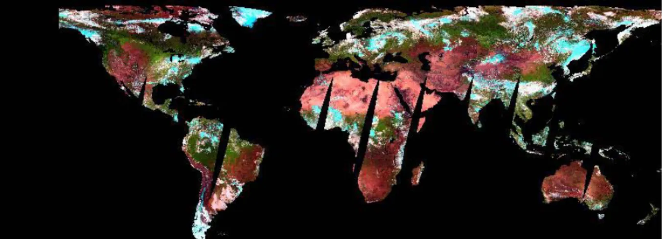
Because of the characteristics of the satellite, repeat acquisitions are made in a single day at moderate to high latitudes in both hemispheres. Where this has occurred the pixel chosen to represent the S1 product is that pixel with the highest normalized difference vegetation index (NDVI) value. This leads to significant speckling in some areas and methods to remove or automatically detect these areas of speckle have proved difficult. Therefore, it was a task of the algorithm development team to ensure their burnt area algorithm was sufficiently robust enough to cope with these overlap regions. It was impossible to retrieve the original data so that just one overpass could be used instead of a composite of both overpasses. Because of the same orbital characteristics mentioned previously, there was not complete daily coverage of the equatorial (90% covered each day, the remaining 10% covered the following day). The maximum off-nadir observation angle of the sensor is 50.5 degrees resulting in a swath width of approximately 2200 km. The imagery were acquired in descending mode at approximately 10:30 local solar time. The S1 product also contained a ‘status’ product that yielded information on the radiometric quality of each pixel and the occurrence of land or water, snow or ice and cloud. However, after discussion with colleagues it became clear that the status map could not be relied upon for providing accurate information to use operationally, for example, to determine the presence of clouds. An example of a global, S1 product is shown in Figure 1. The resampled data is displayed as an RGB image (Red = band MIR, Green = band B3, Blue = band B2). The date of the acquisition is the 30th July 2000.

(13)

Figure 1: Example of a global SPOT Vegetation S1 product acquired on the 30th July 2000. The data is shown as a RGB image (Red = band MIR, Green = band B3, Blue = band B2) and has been resampled to 2% of its original size.

1.1.1 S1 data format

The daily, global datasets were provided in HDF format, each band having its own HDF file that also included information about the calibration and geometry of the data. The method used to extract the data and relevant calibration information (to ground reflectance or angles) from the HDF file is described in Section 2.1. It became clear that the processing was far easier without having to deal with the HDF format when using a variety of software packages and computer code. Each of the S1 products has been resampled to a Plate-Carree projection (with a pixel spacing of approximately 1 km at the equator) using the WGS84 datum as a reference. All of the daily data were co-registered together prior to delivery to the JRC. The main characteristics of the S1 dataset that was used in this project can be summarised by the following points:

• 4 x spectral bands (B0, B2, B3 and MIR) and 4 x angle bands (VZA, VAA, SZA, SAA).

• Each band contained 40320 columns x 14673 lines of data (global coverage).

• The spectral bands are encoded as unsigned 16-bit (integers). To derive the surface reflectance from the digital number (DN), simply multiply the DN by 0.0005.

• The angle bands are encoded as unsigned 8-bit (byte). To derive the value of the angle from the DN, multiply the DN by 1.5 for azimuth angles or multiply by 0.5 for zenith angles (for both viewing and sun angle values).

(14)

• The coordinates of the centre of the upper-left pixel are –180.0 degrees E, 75.0 degrees N.

Uncompressed, a daily dataset occupied 6.6 Gbytes of disk space and there are at least 366 days of data to process (the year 2000 was a leap year). Therefore, effective management of hardware and software resources is a key issue in the execution of this project.

1.2 Utilisation of global land cover products

Information on the land cover at a global scale is useful for the following reasons in the context of the GBA2000 project:

• As a tool to provide data masks of water, urban regions and non-vegetated surfaces such as ice masses and deserts.

• As an information layer used to retrieve statistics of burnt area by land cover (vegetation) type.

• As a guide to utilising burnt area algorithms for detecting burnt areas outside their geographical region where they were developed, but over similar land cover (vegetation) conditions.

A number of global products exist that could have been used. Some of them were developed with a specific application or research area in mind, such as the Simple Biosphere 1 and 2 models (Sellers et al., 1986; Sellers et al., 1996) and some models were too detailed for this application, for example the Global Ecosystems model that has 100 classes (Olson, 1994a; Olson, 1994b). Two models that were considered in this project are the International Geosphere Biosphere Programme (IGBP) land cover classification (Belward, 1996; Belward

et al., 1999) and the University of Maryland (UMD) global land cover product (DeFries et al., 1998; Hansen et al., 2000). After lengthy discussion the IGBP product was rejected. This

was because using two land cover products in the pre-processing stages would be complicated.

1.2.1 UMD land cover product data access and characteristics

All of the data products mentioned in the previous section (apart from UMD product) can be downloaded online, free of charge, from the US Geological Survey (USGS) EROS Data Centre (http://edcdaac.usgs.gov/glcc/glcc.html). The UMD product can be downloaded online, also free of charge, from the UMD Global Land Cover Facility (http://glcf.umiacs.umd.edu/data.html). This website also provides information on the origin

(15)

of the project and the procedure of training the classification model and its validation. The data is available in two projections, either geographic (Plate-Carree) or in Goode’s Homolosine. The geographic projection was chosen at a resolution of 1 km at the equator. The characteristics of the UMD land cover dataset are:

• Image size is 43200 columns x 21600 lines of data. • The data encoding is unsigned 8-bit (byte).

• The projection is geographic based on a sphere of radius 6370997 m. • The pixel spacing equals 0.00833 degrees.

• The coordinates of the centre of the upper-left pixel are –180.0 degrees E, 90.0 degrees N.

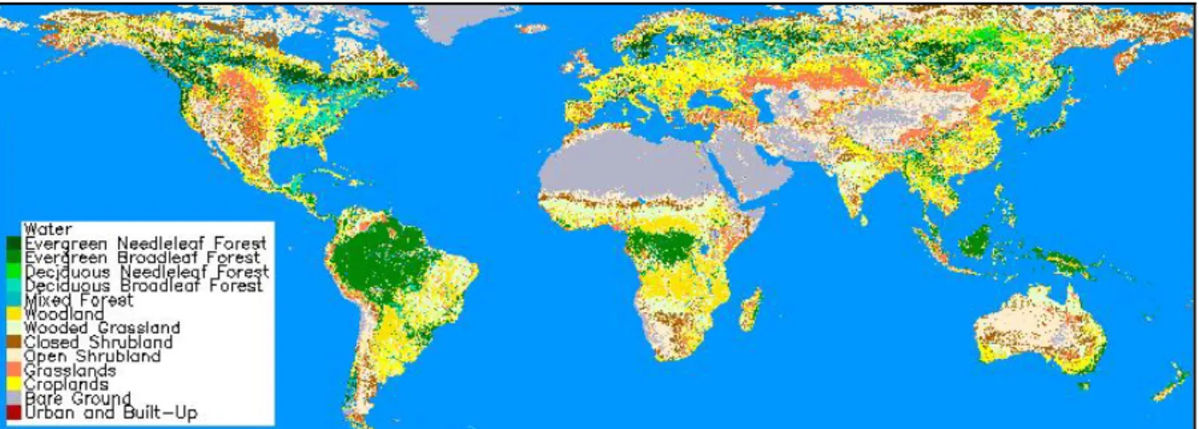
The legend of the UMD land cover dataset is:

Class Value (DN) Class Name 0 Water

1 Evergreen needleleaf forest 2 Evergreen broadleaf forest 3 Deciduous needleleaf forest 4 Deciduous broadleaf forest

5 Mixed forest 6 Woodland 7 Wooded grassland 8 Closed shrubland 9 Open shrubland 10 Grassland 11 Cropland 12 Bare ground

13 Urban and built-up

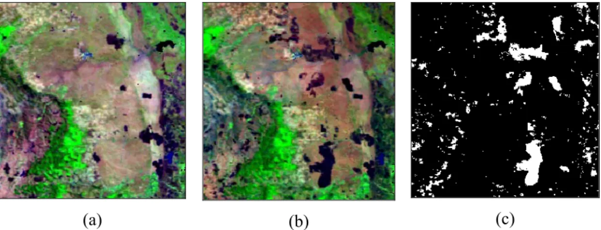
Figure 2 shows the global UMD land cover product, having been significantly reduced from its original size.

(16)

Figure 2: The UMD global land cover product. The image has been resampled to 2% of its original size.

1.2.2 SPOT Vegetation S1 - UMD land cover data co-registration

An initial overlay of the UMD land cover product and the S1 products yielded a significant non-linear offset between the two products that had to be corrected. It was obviously easier to correct the land cover product than all of the S1 products. The commercial software package, ENVI was used to make this correction. In total, 54 tie-points were selected from an S1 product and the UMD land cover product. To perform the correction, a third order polynomial equation was applied to the land cover product with nearest neighbour resampling. The estimated RMS error of the resampling procedure was less than 1 pixel. The resampled land cover product was projected onto the WGS84 datum, with a new pixel spacing of 0.0089285714 degrees and geometry of 40320 columns by 14673 lines (i.e. identical to the SPOT Vegetation S1 data).

1.2.3 Secondary mask products derived from the land cover data

The following secondary products were then derived from the registered UMD land cover dataset:

• A binary mask (0/1), of non-vegetation/vegetation cover. This file would be encoded zero for all classes that were not vegetation (i.e. classes 0 (water), 12 (bare ground) and 13 (urban and built-up)), or otherwise encoded as one.

• A binary mask (0/1), of the vegetation classes that are classified as forest. These are classes 1 (evergreen needleleaf forest), 2 (evergreen broadleaf forest), 3 (deciduous needleleaf forest), 4 (deciduous broadleaf forest) and 5 (mixed forest). This was

(17)

considered useful in case two burnt area algorithms needed to be applied over the same area, one that detects burnt area in forests and the other detecting burnt areas in woodlands, shrublands and grasslands.

• A binary mask (0/1), that satisfied the other vegetated land cover classes that are not forest as described in the previous bullet point.

The storage, accessibility and usage of these products in the GBA2000 project are described in Section 3.5.

1.3 A simplified overview of the main processing tasks

Considerable time was given to thinking about, and formulating the sort of processing needs and requirements of the GBA2000 project. For instance, would there be any common pre-processing requirements that satisfied a number of burnt area algorithms. Would the compositing criteria tested successfully with algorithm A over region B work to provide the required composite data for algorithm C over region D. Initially, the work undertaken by the author, was almost to predict what solutions might be required by the GBA2000 partners and to develop and test some programs with the S1 data. From these early tests and correspondence with GBA2000 partners, it became evident that the algorithms being developed were all very different. They each demanded different amounts of processor time, input data formats and post-processing. However, some of the tasks, mainly in the pre-processing module, were similar or could be approximated by using the same tool. It became clear though that each of the burnt area algorithms would need to be treated separately with only the final results being in a comparable format to enable the final product to be produced. It was decided to break the processing up into several main processing tasks, or modules. The first module is called the data extraction module. After extraction, the data now enters the pre-processing module, containing different sub-routines for each algorithm, followed by entry into the burnt area detection modules. Each of the algorithms provided by the GBA2000 partners require different post-processing algorithms. However, the results are comparable and it is the final task to mosaic the results together to create the global burnt area map of the year 2000. In the following chapters and sections, each module is described in detail.

(18)

1.4 Computing requirements of GBA2000

The majority of the computational processing for the GBA2000 project was achieved using SUN Workstations. Several workstations were utilised so that the processing could be multi-tasked. The workstations used ranged from SUN Ultra 2 with a single processor to a dual processor Ultra 60. The programs were developed so that they could all be run on a system with 128 Mbytes of RAM with an equivalent amount available as swap space. The memory available in the workstations ranged between 128 Mbytes and 1 Gbyte. The amount of disk space available for the project was a limiting factor on the efficiency and productivity of the processing. Obviously, the bigger the disk (or disks) capacity then a larger amount of data can be processed at the same time. The disk space allocated to GBA2000 was approximately 92 Gbytes allocated in partitions of 17.5, 17.5, 10, 34, 9 and 4 Gbytes. It was considered essential that at least one 30+ Gbytes partition was available as this would significantly decrease the processing time of some of the more demanding burnt area algorithms. The operating systems on the SUN workstations are the standard SUN operating system (SUN OS) versions 5.6 and 5.8. All of the disk partitions were cross-mounted with the processors that were available.

The choice of software used to implement the burnt area algorithms were the c programming language, the Interactive Data Language (IDL) developed by Research Systems Inc. (RSI) and the ARC Macro Language (AML) developed by ESRI. This decision was made because of several reasons; the author of this report is familiar with these programming languages, the software was available on the UNIX network at the GVM unit of the JRC, the archived SPOT Vegetation S1 data was accessed through the UNIX network using OS commands, and c-shell scripts could be developed to automate much of the processing. To enable the processing to be undertaken, c language compilers need to be available on the UNIX network (e.g. cc or gcc). Use was made of the standard commands and software available under SUN OS, such as cat, awk, echo, HDF commands and c-shell scripts. Further information about these commands and others can be found in Annex A or by viewing the manual pages on the operating system. The choice of software that the algorithms were written in also depended on the GBA2000 partner that provided the algorithm. In some cases, the algorithm would be provided as a formula or set of equations that the author would encode. In other cases, code would be provided and, if this code was compatible with the UNIX system at the JRC (such as an algorithm by CCRS that was developed in AML from ARC-INFO (see

(19)

http://www.esri.com/software/index.html for details), then the code would be run without any re-writes or changes. It was the job of the author to make the algorithm run automatically. The result is that some of the algorithms are available in the c language, others are in IDL or AML, but they all run on the same system and executed in the same way (i.e. using c-shell scripts). A brief description of the use of c-shell scripts is now given.

1.4.1 Automating the processing using c-shell scripts

The use of c-shells, or any shell environment, to automate processing and tasks is well practiced. By using this software, that is standard on SUN OS, it is possible to keep the processing modules discrete from each other, keep programs from becoming too long and complicated and also allow easy bug fixing if the processing goes wrong. Additional, advantages of c-shell scripts are that tasks can easily be repeated many times and that c programs can be executed automatically as well as IDL programs and AML modules within ARC-INFO. A c-shell script is a simple text file that is interpreted by the operating system as a script with the inclusion of the following information on the first line:

#! /bin/csh –f

This tells the operating system that the text file is a c-shell script. The text editor used to develop these programs is called, nedit (the author strongly encourages the use of this editor, or another editor of similar quality, for all text editing). A c-shell script is basically a series of commands that are executed in sequence after the previous command has finished. Within the c-shell it is possible to repeat commands within loops, assign variables from command line input values, direct input and output (using, < and >), make simple mathematical calculations and assign text and numerical variables from text files using the commands, awk and sed (type, man awk or man sed for more information). Other manipulations are available. Also, if the code is made generic so that specifics are given at the command line that activates the c-shell script, then they can be run anywhere within the directory structure. Examples of c-c-shell scripts that illustrate the points made above are given in Annex A.

1.4.2 Location of executable binaries and source code

To avoid replication of command files in multiple directories, it is possible to store all of the binaries (c programs, c-shell scripts, awk programs) within one directory. In the GBA2000 project, necessary files were located in ~tanseke/bin, where ~tanseke, refers to the location of

(20)

then added to the list of those directories looked in when executing commands in the .cshrc file located in the user’s home directory (please consult your system administrator or technician for information about this file). The source files of the c programs were kept separately in the directory called ~tanseke/src. A directory called ~tanseke/src/idl contained the IDL programs. The IDL programs are not compiled before use, rather that is done automatically when the program is called. Therefore, before these programs are called, they are copied from this central resource to the working directory (i.e. where the processing is taking place). After the processing is complete, the copy is deleted. The AML programs are located in a central resource, in this case ~tanseke/src/amls. These files can be called and run from this directory without the need to copy the program to the working directory. Also, directories ~tanseke/bin/text and ~tanseke/bin/img have been created that respectively contain important text and image files, required at certain times during the processing.

1.4.3 Computational processing demands geographical area relationships

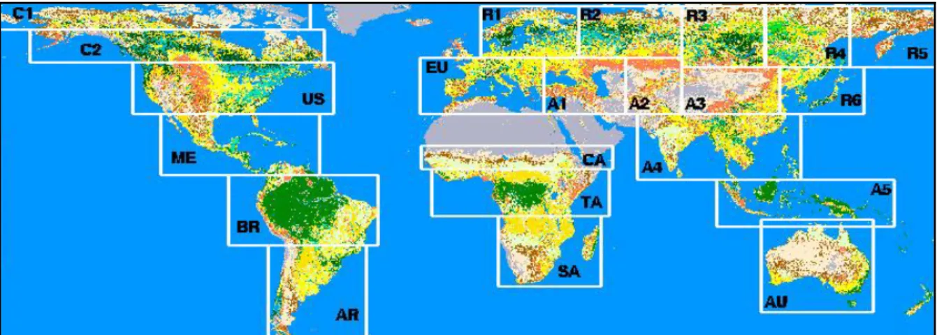
The large size of the SPOT Vegetation S1 global dataset and the development of regional algorithms ensured that the processing would be undertaken on a regional scale. During early considerations of the processing tasks, it was considered that all of the algorithms could be applied to all of the geographical regions without causing a software or hardware failure on any of the systems available. This was achieved, even if some of the processes would be extremely slow on the older machines. So, based in part on the processing demands of the algorithms (and in some part on the land cover zoning and the physical shape of the land surfaces), the global dataset was divided into regions of interest (sub-windows). The method of extracting the sub-windows is presented in Section 2.5.2. Figure 3 shows these regions of interest and the acronym given to each of these.

(21)

Figure 3: Division of the global dataset into regional sub-windows, imposed because of hardware and software processing limitations. An acronym is given for each sub-window.

Note in Figure 3 that New Zealand, Greenland and sections of the Middle East and the UK were not processed. The low occurrence of vegetation burning in these regions caused by a lack of vegetation or burning regulations made the processing of these areas unnecessary.

1.4.4 Further software requirements

Other software tools that were utilised in the GBA2000 project were the Environment for Visualising Images (ENVI), by Research Systems Inc., a tool that is based on the Interactive Data Language (IDL) and programs of ARC (ARC-VIEW, ARC-INFO and ARC-GRID) by Environmental Systems Research Institute Inc. ENVI is commercially available software that provides tools for the display and manipulation of data. This software was used mainly for the display and viewing of image files, overlay of vector information, creation of maps for printing and projection of Plate-Carree data to equal area projections. Using ENVI to display images requires that a header file with the same file name (but with the extension .hdr) is available (if not one is created). A feature of many of the GBA2000 programs is the automatic creation of the ENVI header of the binary image data, so that these images can be displayed quickly in ENVI. The ENVI header file, in its basic form, is a simple text file that provides geometrical and geographical information. The header file provides information on any type of binary image, for example the global land cover products, which are effectively classifications with a legend. The structure of the ENVI header file is described in Annex A and two examples are given. Even if you do not utilise ENVI, the header file still provides useful information about the image file. The versions of ENVI and IDL used were 3.4 and 5.4.1 respectively.

(22)

The programs available within ARC were used to create ARC Grids from the binary image data (burnt areas and land cover products) and projection to equal area (INFO or ARC-GRID command). The AML was used for a burnt area algorithm, described in Chapter 9, where complete description of the commands used to derive the burnt are products are presented. The versions of ARC and ARC-VIEW used were 8.0.1 and 3.2 respectively.

1.5 Utilisation of digital elevation model (DEM) data

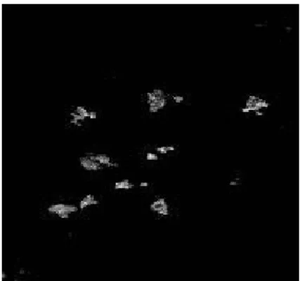
During the processing of the GBA2000 SPOT Vegetation S1 dataset, in the regions of the Himalayas and the Andes mountain ranges large regions of possible burnt areas were detected by the algorithms used in these regions. After closer inspections of the results were made, it was believed that these areas were being mistaken as being burnt because these areas were lying in the sun’s shadow during certain times of the year and this would affect the pixel’s spectral reflectance. The drop in reflectance would, in some cases, be falsely interpreted as being a burnt area. The regions identified as needing attention were the Andes mountain range of South America (windows ME, BR and AR in Figure 3) and the Himalayas mountain range (window A4 in Figure 3). It was necessary to determine those pixels that could be affected by the sun shadow at different months of the year. To achieve this, a DEM was needed.

After a search of the Internet of available global DEM’s, the Global Land One-km Base Elevation (GLOBE) product was used (Hastings and Dunbar, 1998; see also http://www.ngdc.noaa.gov/seg/topo/globe.shtml). The DEM data can be downloaded by geographical region from the Internet. In addition, a layer corresponding to the source of the DEM is available. The data format is signed 16 bit and the byte order is INTEL (little-endian). The individual tiles for two regions were joined together using IDL ENVI software. These two regions were Central and South America and the Indian subcontinent, continental south-east Asia and insular south-east Asia. The projection of the GLOBE data is geographic (degrees) and the pixel size is 0.008333333 degrees. Because of the small difference in pixel size between the SPOT Vegetation S1 products and the DEM product, the DEM product was resampled to the pixel size of the image data. A visual confirmation of a good match was made. Any form of accurate co-registration was impossible given the types of data being used. For each of the regions of interest, where it was thought that sun shadow might lead to false detections, a subset of the DEM was extracted. These regions were ME (Mexico), BR

(23)

(Brazil), AR (Argentina) and A4 (India, China and south-east Asia). The use of a DEM was not considered necessary for window A5 (insular south-east Asia).

1.5.1 Determining sun shadow affected pixels

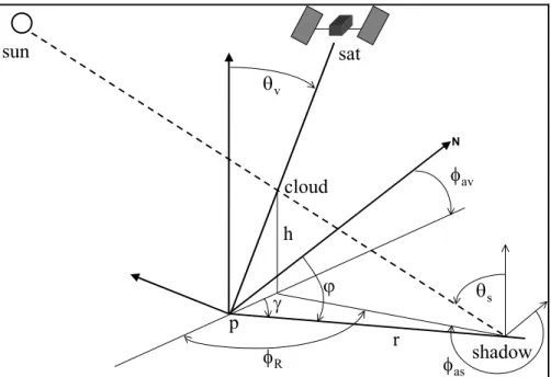
The method used to determine pixels that are contaminated by sun shadow is given by Colby (1991). The cosine of the solar incidence angle is determined by the following equation: cosi = cos θs cos θn + sin θs sin θn cos (φs – φn)

where, cosi is the cosine of the solar incidence angle, θs is the sun zenith angle, θn is

the terrain slope, φs is the sun azimuth angle and φn is the terrain aspect.

To derive the terrain slope and aspect, IDL ENVI software was used (note that this task can be performed by most commercial image analysis software). The slope and aspect products were derived over a 3x3 window and assuming a pixel size on the ground of 1km. Given the time constraints of the project, there was insufficient time to undertake a sensitivity analysis of the optimum threshold to apply to the cosine of the solar incidence angle to indicate that a pixel is affected by sun shadow. After some brief tests were conducted in the Andes of South America a value of 0.5 for the cosine of the solar incidence angle was chosen. This means that if the incidence angle of the solar radiation on the surface representing each pixel was below sixty degrees then this pixel would be indicated as being contaminated by sun shadow. The sun zenith and azimuth angle information is derived from the SPOT Vegetation S1 products on a daily basis.

A c program was written that made the calculations shown in the equation above. To enable the threshold value to be changed by the user, this parameter was made an input variable at the command line. A c-shell script was written to automatically produce sun shadow contamination masks for any time period.

It was decided to use these masks in the post-processing stages of the GBA2000 project. This was mainly because, the user needed to determine whether or not the application of these masks to the final burnt area maps was actually necessary. Therefore, this meant that sun shadow masks that indicated all of those pixels that were contaminated for the whole of the month under consideration (and not just the each day). For example, pixels not contaminated

(24)

monthly burnt area product is presented then all of those pixels possibly contaminated by sun shadow during the whole of that month must be removed. Finally, for some of the algorithms, tests are made between images (or composite images) acquired over two months. In this case, all contaminated pixels in both months must be considered.

1.5.2 Sun shadow masking procedure

The procedure adopted by the GBA2000 project was to determine the contaminated pixels for each daily image set over a time period of one month using a sun incidence angle cosine value of 0.5. Because of the assumptions made of the pixel size and accuracy of the DEM product, the sun shadow masks were eroded by one pixel in all directions. Although this resulted in a loss of data, it was considered a necessary step after observations of the results in the Andes test area. The daily masks for each month were then multiplied together to obtain a single mask for each month indicating all contaminated pixels. Where tests were made over a two month period to determine burnt areas, these monthly products for these two months would be multiplied together to derive a bi-monthly mask. The DEM derived products (slope and aspect images) are located in a directory called dem_products located in the working directory of each region of interest (e.g. ./BR/dem_products).

The c-shell script gba_sun_shadow_mask.csh has been written to automate the production of the monthly sun shadow masks. The syntax of the script is:

###################################################### GBA2000 C shell: gba_sun_shadow_mask.csh

Copyright JRC, 2001

Contact person: kevin.tansey@jrc.it

######################################################

Syntax: gba_sun_shadow_mask.csh <acronym>

<apply mask to data to which level (0 or none, vza, mir, cloud, cl_comp, shadow, burn, basic or all)> <cosine of sun incidence angle threshold (e.g. 0.5)>"

<dilate sun incidence angle mask by 1 pixel (0 = no, 1 = yes)>" <delete mask (1,0) files (1 = yes, 0 = no)>"

where, the acronym is the two letter window code, the apply mask parameter indicates to the program the level of pre-processing that the user requires to be composited (the codes point the program to the correct input files that have been produced by the pre-processing algorithms presented in Chapter 3 and a zero here indicates that original S1 data is to be processed), the threshold value of the cosine of the solar incidence angle is stated, a flag value stated to indicate if the user would like to erode (or dilate) the sun shadow masks in each direction by one pixel and the final parameter indicates that the user would like to delete

(25)

the daily masks and also a file containing values of the cosine of the solar incidence angle. Further details of this program are given in Annex A.

The script calls a c program called sun_shadow_mask.c. The inputs to this program are the following:

sun_shadow_mask

terrain aspect image (float) terrain slope image (float) sun azimuth angle image (byte) sun zenith angle image (byte)

output cosine of solar incidence angle image (float) output sun shadow mask image (byte)

$pixels $lines

cosine of solar incidence angle threshold

A full description of this program is given in Annex A.

After a sun shadow contamination mask has been produced for each day, a monthly product is produced using the generic c program apply_mask.c (Annex A). This file is written to a directory named sun_shadow_masks located in the working directory of the region of interest. Where GBA2000 algorithms utilise these sun shadow masks then this is described in the post-processing section of the individual algorithm descriptions contained within this report.

(26)

2 Data extraction from tape archive

The daily, global S1 image dataset acquired between 1st December 1999 and 31st December 2000 is stored on tape archive within the GVM Unit. The data on the tape archive can only be accessed by a limited number of users at the same time, and two users cannot access the same tape at the same time. The amount of data available is huge and, for obvious reasons, cannot all be accessed for processing at the same time. Therefore, programs were developed so that specific regions of the globe and specific dates could be retrieved from the archive and presented in an orderly manner automatically. This chapter first describes the format of the archived SPOT Vegetation data, then outlines the programs required to extract a particular region of interest for a particular time period in sections two and three. The extraction of land cover information is covered in the fourth section. The fifth section describes a special case that is considered when extracting the image data for some regions of the globe. The final section lists the daily datasets that have problems associated with them (i.e. missing days, different file names, missing data etc.).

2.1 Data format of original SPOT Vegetation S1 archived products

The original S1 products are located in the remote directory:

/gvmarchive/vgtglday$month$year/$year$month$day

where, the variables pre-fixed by a dollar sign ($) indicates the year (e.g. 2000), month (e.g. 11) and day (e.g. 23) of acquisition.

Inside this directory, the following files are available (example is shown for the 15th_June

2000): ./0001_b0.zip ./0001_b2.zip ./0001_b3.zip ./0001_log.zip ./0001_mir.zip ./0001_ndv.zip ./0001_ql.zip ./0001_rig.zip ./0001_saa.zip ./0001_sm.zip ./0001_sza.zip ./0001_tg.zip ./0001_vaa.zip ./0001_vza.zip

(27)

This file naming convention is the same for each of the daily datasets, hence, it is important when retrieving the data to keep track of which date the file represents. The author refers the reader to the SPOT Vegetation data manual for a more complete description of the content of the files stated above (available at http://vegetation.cnes.fr). The files that are important to the GBA2000 project are those with the extensions b0, b2, b3, mir, saa, sza, vaa, vza and log. The first four files contain the spectral information, the next four files contain the angular information and the final file (log) contains geometric, cartographic and projection information.

To save disk space each file has been compressed. When decompressed, the spectral and angular images have the extension .HDF. The data is in Hierarchical Data Format (HDF) (see http://hdf.ncsa.uiuc.edu/ for more details). This data format is very useful when multiple files and meta-data information need to be structured in such a way that they are contained within the same file, such as with Landsat TM data. However, in this case there is only a single band of information contained within each HDF file and the geometry (columns and lines) of this single file is always known. In addition, most of the meta-data contained within the HDF file is not required by the GBA2000 project. Furthermore, image manipulation with HDF files makes processing far more complicated. Given all of these factors, it was decided that, when extracting the region of interest from the data archive, firstly the image files would renamed to something that could easily be associated with the region of interest (by using an acronym) and the date of image acquisition (giving the file a date code), second, the image data would be extracted from the HDF file and written as simple BSQ (band sequential) file with no internal header information, and third, writing the files to a directory structure that enables the user to easily understand and locate data products from their location within the directory. The structure of the directory to which the extracted datasets were written was made up of a root directory that was named after a two-letter acronym given to each of the geographical regions (e.g. AU refers to Australia). All of the geographical regions analysed by the GBA2000 project are shown in Figure 3 along with their acronyms. In the case for Russia, the country was divided into several sections, numbered consecutively. As the files were extracted for each date requested, a sub-directory would be created (inside the root directory), of the form $year$month$day (e.g. 20000615). Inside each of the sub-directories would be written the image data, angular data and calibration information, for that day and for that

(28)

particular geographical region identified by the acronym preceding the date, as shown below (example of Australia is given):

./AU/20000614/… ./AU/20000615/AU_20000615_b0 ./AU/20000615/AU_20000615_b2 ./AU/20000615/AU_20000615_b3 ./AU/20000615/AU_20000615_mir ./AU/20000615/AU_20000615_saa ./AU/20000615/AU_20000615_sza ./AU/20000615/AU_20000615_vaa ./AU/20000615/AU_20000615_vza ./AU/20000615/20000615_log.txt ./AU/20000615/20000615_calib_par.txt ./AU/20000616/…

where, the log and calibration parameter files are in ASCII text format and provide metadata information for projecting and calibrating the spectral data.

This data structure is understood by programs developed by the author for processing the SPOT Vegetation dataset into a burnt area product.

2.2 Controlling the time period of analysis: input_dates.txt

The text file named input_dates.txt is absolutely critical for controlling the GBA2000 processing. It is evident that for many regions of the globe the occurrence of vegetation fires is during a specific time period. Therefore, it is pointless trying to retrieve data spanning the whole of year 2000, if there are no burnt areas to detect. Information on the timing of burning in different regions of the globe was obtained from discussion with local experts, reading literature on the subject and examining images from a range of dates throughout the year. It was also a waste of computing resources to process data that do not contain any burnt areas. Literature on the timing of vegetation fires has been well published (Dwyer et al., 1998, 1999; Barbosa et al., 1999). To control the range of dates that the user needs to process, a text file is used. An example of the text file is:

# Input file listing dates for processing of the GBA product # Input year, month and days you want to process

years = 2000 months = 07 # days = 21

# For full image processing use these value # years = 1999 2000

# months = 01 02 03 04 05 06 07 08 09 10 11 12

(29)

The file is named input_dates.txt and a copy should always be available in a central resource (e.g. ~<user>/bin/text/). Copy the file to the current working directory (e.g. ./AU) and edit the file using a suitable text editor (e.g. nedit). All of those lines that begin with a hash symbol (#) are ignored. The details are repeated so that the lower sets of values are given to represent the whole dataset, i.e. all days in all months in all years. The upper set of values can be altered and modified according to the user’s requirements. By copying and pasting values from the lower set of values into the upper set of values mistakes cannot be made. In the example shown, a program that needs temporal information, when activated at the command line will read in the file, input_dates.txt and see that it needs to process each day in the month of July (month 07) for the year 2000 dataset. Programs will test for the presence of this file within the working directory and may fail if this file is not located.

2.3 Extracting SPOT Vegetation S1 data from tape archive

A c-shell script, that calls a number of c programs, is the method used to extract the data, for a specified region, from the archive. The script then renames the files and strips the HDF structure from the original SPOT Vegetation S1 products. The script also extracts for the same geographical region the UMD land cover products and masks that are described in Section 2.4. To retrieve a specific geographical region, the location of the region (or window) must be known in terms of pixels offset in columns and lines relative to the start position (0, 0) of the upper-left pixel. The coordinate (0, 0) is chosen as this is better represented in c-shell and c programming. This can be calculated in several ways either by looking at the global product and determining the map pixel offset in columns and lines or using the geometry of the file, given the geographical coordinates of the window and the pixel spacing in degrees. The offset, measured in pixels, of the upper left corner of the region of interest, compared to 0, 0 of the global product. For example, the Australian dataset is offset 32702 columns (also known as pixels) and 9519 lines relative to the global product. In the extraction program, these offsets are termed x_start and y_start respectively. The user needs to know the size of the geographical dataset, also in terms of columns (pixels) and lines. Using Australia again as an example, the size of the window is 4817 columns (pixels) by 3921 lines. In the extraction program, these parameters are known as x_size and y_size respectively. The program initially checks a list of pre-defined regions of the globe. This list is in the form of a text file that is located in a central resource. The list of regions is called gba_country_list.txt and is located in the directory, ~<user>/bin/text. An extract of that list is now shown.

(30)

# List of GBA2000 Regional Sub-windows # Legend is:

# country_name acronym x_start y_start x_size y_size # Regional Sub-Windows australia AU 32722 9539 4777 3881 canada1 C1 20 20 13400 1380 canada2 C2 1400 1400 12600 1400 usa US 5800 2800 8600 2200 mexico ME 7000 5000 6800 2600 brazil BR 9900 7600 6400 3000 argentina AR 11600 10600 4200 4000 c_africa CA 18150 6350 8200 1000 t_africa TA 18600 7350 7600 2000 s_africa SA 21450 9350 4400 3000 europe EU 18100 2600 5400 2400 russia1 R1 20700 400 4200 2200 russia2 R2 24900 400 4400 2200 russia3 R3 29300 400 3600 2600 russia4 R4 32900 400 3600 2600 russia5 R5 36500 400 3800 2600 russia6 R6 33500 3000 3600 2000 asia1 A1 23500 2600 3400 2400 asia2 A2 26900 2600 2400 2400 asia3 A3 29300 3000 4200 2000 asia4 A4 27400 5000 7000 2800 asia5 A5 30800 7800 7600 2000

The first column of data is matched with the input variable given, the second column is the acronym given to the sub-window and the following four columns indicate the location and the size of the sub-window relative to the global product. This file can be added to and edited to suit the requirements of the user

The c-shell script gba_read_vgt_data.csh is available to perform all of the tasks outlined above in an automated way. To extract a dataset, essentially all the user has to do is edit the file, input_dates.txt for the required time period, and specify either one of the listed GBA2000 processing windows (e.g. the first section of Canada, C1 or Australia, AU) or specify the input parameters (x_start, y_start, x_size and y_size) and provide an acronym for the geographical region (e.g. IT for Italy) and run the program. By specifying more detail at the command line when running the program, it is possible to extract land cover information and/or retrieve the geographical region, buffered by twenty pixels to provide better cloud shadow detection results. These add-in’s to the main program are discussed in Section 2.5. If the user types gba_read_vgt_data.csh at the command line instructions appear on how to use the program. A description of the procedures followed by the script is now given, a more complete description and the code of the script is given in Annex B.

(31)

###################################################### GBA2000 C shell: gba_read_vgt_data.csh

Contact person: kevin.tansey@jrc.it

###################################################### Syntax: gba_read_vgt_data.csh

<acronym> <x_start> <y_start> <x_pixels> <y_lines> Notes:

Copy and edit the file '~tanseke/bin/text/input_dates.txt' to the current directory Edit the file '~tanseke/bin/text/gba_country_list.txt.txt'

Select from:

globe = global product (GL) GBA2000 continental datasets: australia = continental Australia (AU)

canada1 = Canadian far northern latitudes (C1) canada2 = Canadian northern latitudes (C2) usa = United States of America (US) mexico = Mexico and Central America (ME)

brazil = Brazilian Amazon and northern S. America (BR) argentina = southern S. America (AR)

c_africa = central Africa (CA) t_africa = tropical Africa (TA) s_africa = southern Africa (SA) russia1 = European Russia (R1) russia2 = west Asian Russia (R2) russia3 = central Asian Russia (R3) russia4 = eastern Asian Russia (R4) russia5 = far east Asian Russia (R5) russia6 = south-east Russia and Japan (R6) europe = southern and central Europe (EU) asia1 = Black Sea, Turkey and Middle East (A1) asia2 = central Asia (A2)

asia3 = northern China and Mongolia (A3)

asia4 = Indian sub-continent and mainland southern Asia (A4) asia5 = Insular south-east Asia (A5)

Flag extract land cover = 1 to retrieve UMD window

Flag apply pixel buffer = 1 to make buffer (value set in this program)

Otherwise enter 'other' for country, acronym and coordinates of the image sample

Initially, we will ignore any extraction of land cover images. So, entering the command:

gba_read_vgt_data.csh russia3 0 1

This will tell the program that you want to extract the window russia3 with no corresponding land cover information but with a buffer of twenty pixels. Inside the file gba_country_list.txt parameters for the acronym, global offset and size of the window of region russia3 are listed. In another situation, the user could enter the command:

gba_read_vgt_data.csh other 0 0 MD 24980 9730 850 1560

This will tell the program that you want to extract a window that is not listed in the country list text file, by defining the input parameter as, other. The user also does not want to extract

(32)

window (second flag set to zero). The user has defined the acronym MD for this region of interest. The offset in pixels from the upper-left corner of the global product is 24980 columns (pixels) and 9730 lines. The size of the region of interest is 850 columns (pixels) by 1560 lines. This area corresponds to the country of Madagascar.

On execution of the command for any region of interest the procedures that are activated are approximately the same, and therefore can be described in general terms. An example is given for extracting data files covering the Australian (AU) window. The first step is to test for the presence or absence of files. These include the file input_dates.txt and the remote directory on the tape archive containing the image data for the date that is being extracted. If the directory does not exist for that day then the program moves onto the next date in the input_dates.txt file. In this example, the data for the date of interest is available (15th June 2000) and a directory $year$month$day is created in the working directory (e.g. ./20000615). The file 0001_log.zip is copied to a temporary directory (./temp_hdf) and uncompressed using the command unzip. The file is renamed and placed in the date directory recently created (e.g. ./20000615/20000615_log.txt). An example of this log file can be found in Annex B. A file called ./20000615/20000615_calib_par.txt is then created using the SUN OS command echo. This file will contain the calibration factors for the spectral bands and angular bands for this particular date. This information is contained within the metadata of the HDF files.

The program now repeats the following procedure for the four spectral bands (of type integer) and the four angle bands (of type byte). The procedure is described in detail for the MIR band. The data, in a compressed format, is copied from the tape archive to a temporary directory. The file is then decompressed and renamed within the temporary directory with the following form, for example ./temp_hdf/20000615_mir.hdf. The HDF file needs to be analysed to locate the position within the HDF file of the data to be extracted in BSQ format and also the calibration information. The program calls a small c-shell script gba_read_hdf.csh to interpret the structure of the HDF file. This c-shell script is activated at the command line with the command:

(33)

gba_read_hdf.csh

temp_hdf/$year$month$day_$image.hdf >> temp_hdf/$image.hdf.txt

where, the variable image in this case refers to the band being processed (e.g. MIR) and the >> indicates that the output from the c-shell script should be redirected into a text file, in this example to mir.hdf.txt.

When the c-shell script gba_read_hdf.csh is activated it calls a special command that is able to interpret the HDF file. These commands are usually available on the SUN OS (or can be downloaded from HDF websites, see http://hdf.ncsa.uiuc.edu/). The command used for this purpose is hdfed (i.e. HDF editor). By associating input parameters with this command it is possible to print to a text file, information on the location (byte offset) and size (number of bytes) of files within the HDF file. More information and the code for this c-shell script are given in Annex B. An example of the output text file created is:

(1) Version Descriptor : (Tag 30) Ref: 1, Offset: 202, Length: 92 (bytes) (2) Vdata Storage : (Tag 1963) Ref: 2, Offset: 294, Length: 120 (bytes) (3) Vdata : (Tag 1962) Ref: 2, Offset: 414, Length: 85 (bytes) (4) Vdata Storage : (Tag 1963) Ref: 3, Offset: 499, Length: 240 (bytes) (5) Vdata : (Tag 1962) Ref: 3, Offset: 739, Length: 90 (bytes) (6) Scientific Data : (Tag 702) Ref: 5, Offset: 829, Length: 1183230720 (bytes) (7) Vdata Storage : (Tag 1963) Ref: 6, Offset: 1183231549, Length: 4 (bytes) (8) Vdata : (Tag 1962) Ref: 6, Offset: 1183231553, Length: 60 (bytes) (9) Vdata Storage : (Tag 1963) Ref: 7, Offset: 1183231613, Length: 58692 (bytes) (10) Vdata : (Tag 1962) Ref: 7, Offset: 1183290305, Length: 60 (bytes) (11) Vgroup : (Tag 1965) Ref: 8, Offset: 1183290365, Length: 37 (bytes) (12) Vdata Storage : (Tag 1963) Ref: 9, Offset: 1183290402, Length: 4 (bytes) (13) Vdata : (Tag 1962) Ref: 9, Offset: 1183290406, Length: 60 (bytes) (14) Vdata Storage : (Tag 1963) Ref: 10, Offset: 1183290466, Length: 161280 (bytes) (15) Vdata : (Tag 1962) Ref: 10, Offset: 1183451746, Length: 60 (bytes) (16) Vgroup : (Tag 1965) Ref: 11, Offset: 1183451806, Length: 37 (bytes) (17) Vdata Storage : (Tag 1963) Ref: 12, Offset: 1183452041, Length: 4 (bytes) (18) Vdata : (Tag 1962) Ref: 12, Offset: 1183452045, Length: 61 (bytes) (19) Number type : (Tag 106) Ref: 13, Offset: 1183452106, Length: 4 (bytes) (20) SciData dimension record : (Tag 701) Ref: 13, Offset: 1183452110, Length: 22 (bytes) *(21) Numeric Data Group : (Tag 720) Ref: 4, Offset: 1183452132, Length: 16 (bytes) (22) Vgroup : (Tag 1965) Ref: 14, Offset: 1183452148, Length: 59 (bytes)

(34)

From the geometry of the global dataset and knowing the number of bytes per pixel, we know what the total number of bytes that the image occupies. In the case of the spectral data this is, 40320 multiplied by 14673 and multiplied by 2 = 1183230720 bytes and half of this value for the angular data. If we look at the example shown above we can see this value within the file (shown in bold type). On the same line as this value is another value indicating the offset (in bytes) to the image. To summarise, from this text file, we know the size and characteristics of the BSQ image we would like to extract, and the offset to the beginning of the data within the HDF file. In addition, we have already established the pixel offset (in columns and lines) from the global dataset to the regional dataset that we want to extract. Therefore, we can use the generic c program snip.c (Annex A) to extract from the HDF file the exact region of interest without firstly extracting the global BSQ file and then extracting the smaller region of interest. The program checks for the value of 1183230720 in the 6th column (in this case, a column is separated by a white space) and then reads to a variable the value in the 4th column (the offset which in this example is 829 bytes). In the case of the angular data the value looked for in the 6th_{column is 591615360.}

For data calibration, details provided by documentation from SPOT IMAGE, indicated that the information required is located in a section with length 240 bytes as shown above in bold type. Again the offset to this section of the file was written to a variable. This section of the data was extracted first using the generic c program snip.c:

snip temp_hdf/$year$month$day_$image.hdf

temp_hdf/cal_values_$image.txt 100 100 0 0 240 1 $cal_offset 1

where, the variable cal_offset is the offset in bytes to the calibration information section of the HDF file.

All 240 bytes of information are extracted from the HDF file and written to a text file. This file is then analysed and the calibration parameters extracted using commands based on awk (see the manual pages on the SUN OS for a description of awk). These parameters are then written to the file called $year$month$day_calib_par.txt. After all the bands have been processed resembles this example from the 15th June 2000:

(35)

Calibration Parameters for Spectral Bands and Sun/Viewing Angles (date=20000615) ---

####################################################### Formula:

real_val (reflectance or angle in degrees) = a * DN + b

####################################################### b0 calibration coefficient 'a' = 0.0005

b0 calibration coefficient 'b' = 0.0 b2 calibration coefficient 'a' = 0.0005 b2 calibration coefficient 'b' = 0.0 b3 calibration coefficient 'a' = 0.0005 b3 calibration coefficient 'b' = 0.0 mir calibration coefficient 'a' = 0.0005 mir calibration coefficient 'b' = 0.0 saa calibration coefficient 'a' = 1.5 saa calibration coefficient 'b' = 0.0 sza calibration coefficient 'a' = 0.5 sza calibration coefficient 'b' = 0.0 vaa calibration coefficient 'a' = 1.5 vaa calibration coefficient 'b' = 0.0 vza calibration coefficient 'a' = 0.5 vza calibration coefficient 'b' = 0.0

Even though the calibration constants remained the same for S1 products this exercise is useful to ensure that no alternative values exist for the whole dataset.

To extract the specified region of interest, the program again uses the c program snip.c:

snip temp_hdf/$year$month$day_$image.hdf

$year$month$day/$acronym_$year$month$day_$image $global_pixels $global_lines $x_start $y_start $x_pixels $y_lines $offset $bytes_per_pixel

where, the values of x_start, y_start, x_size and y_size come from the parameters of the region of interest outlined previously. The variable offset is the value of the number of bytes from the beginning of the HDF file to the location when the data begins and the variable, bytes_per_pixel is given a value of two for the spectral data (integers) and one for the angle data (bytes).

The output file is written to the date directory created previously and is called ./20000615/AU_20000615_mir. A header file is then created, the ENVI software can immediately interpret that. The format of this header file is described in Section 1.4.4 and in Annex A. To enable the projection information to be written to the header file of the region extracted, new geographic coordinates of the upper left pixel need to be calculated. This is done using the generic c program new_coordinates.c (Annex A). The command to calculate the new longitude and then the new latitude of the upper left corner of the region of interest

(36)

new_coordinates $top_left_lon 0 $x_start $pixel_size > temp_new_coordinate_lon new_coordinates $top_left_lat 1 $y_start $pixel_size > temp_new_coordinate_lat

where, the top_left_lon is the longitude value of the global dataset (i.e. –180.0), the zero (0) flag indicates that the calculation is being made for longitude (as opposed to one (1) for latitude in the second command), the value of x_start indicates the offset in columns (in units of pixels) to the region of interest and the pixel_size is the pixel spacing of both products (in decimal degrees). The same is true for calculating the new latitude value.

The new coordinates are written to the header file. The procedure is then repeated for four spectral bands and four angle bands.

The final stage of the extraction program (after the extraction of all dates listed in the control file input_dates.txt) is to write out to the working directory a text file containing important information that is referred to in later stages of the GBA2000 project. This file is called $acronym_file_info.txt, where the acronym indicates the region that is being processed (e.g. ./AU_file_info.txt for Australia). In later stages of processing, the presence of this file is tested for, and many programs will not run without this file being available. Therefore, it is important that this file is created either using this c-shell script or created using your own text editor. An example of this text file is now shown for the Australian sub-window (./AU_file_info.txt). acronym = AU global_x_offset = 32702 global_y_offset = 9519 samples = 4817 lines = 3921 start_lon = 111.982142 start_lat = -9.991071 pixel_size = 0.0089285714

The file contains information on the relative position of the Australian sub-window within the global dataset, the number of samples (equal to columns and pixels) and lines of the sub-window, the geographic coordinates of the upper left pixel and the pixel spacing. The program is now finished and returns to the command line.

2.4 Simultaneous extraction of registered UMD land cover information

By selecting the necessary flag when implementing the c-shell script gba_read_vgt_data.csh it is possible to extract registered UMD land cover and mask products for the specified region of interest. For example, enter the command: