Measurement of jet activity produced in top-quark events with an electron, a muon and two $b$-tagged jets in the final state in $pp$ collisions at $\sqrt{s}=13$ TeV with the ATLAS detector

EUROPEAN ORGANISATION FOR NUCLEAR RESEARCH (CERN)

Eur. Phys. J. C77 (2017) 220

DOI:doi:10.1140/epjc/s10052-017-4766-0

CERN-EP-2016-218 11th May 2017

Measurement of jet activity produced in top-quark

events with an electron, a muon and two b-tagged

jets in the final state in pp collisions at

√

s

= 13 TeV

with the ATLAS detector

The ATLAS Collaboration

Measurements of jet activity in top-quark pair events produced in proton–proton collisions are presented, using 3.2 fb−1of pp collision data at a centre-of-mass energy of 13 TeV collec-ted by the ATLAS experiment at the Large Hadron Collider. Events are chosen by requiring an opposite-charge eµ pair and two b-tagged jets in the final state. The normalised di fferen-tial cross-sections of top-quark pair production are presented as functions of additional-jet multiplicity and transverse momentum, pT. The fraction of signal events that do not contain additional jet activity in a given rapidity region, the gap fraction, is measured as a function of the pTthreshold for additional jets, and is also presented for different invariant mass regions of the eµb¯b system. All measurements are corrected for detector effects and presented as particle-level distributions compared to predictions with different theoretical approaches for QCD radiation. While the kinematics of the jets from top-quark decays are described well, the generators show differing levels of agreement with the measurements of observables that depend on the production of additional jets.

c

2017 CERN for the benefit of the ATLAS Collaboration.

Reproduction of this article or parts of it is allowed as specified in the CC-BY-4.0 license.

Contents

1 Introduction 3

2 ATLAS detector 4

3 Data and simulation samples 4

4 Object reconstruction 6

5 Event selection and background estimates 7

6 Sources of systematic uncertainty 11

7 Definition of the fiducial phase space 12

8 Measurement of jet multiplicities and p_Tspectra 12

8.1 Jet multiplicity results 15

8.2 Jet pTspectra results 16

9 Gap fraction measurements 24

9.1 Gap fraction results in rapidity regions 25

9.2 Gap fraction results in meµbbsubsamples 31

1 Introduction

Top-quark pair production final states in proton–proton (pp) collisions at the Large Hadron Collider (LHC) often include additional jets not directly produced in the top-quark decays. The uncertainties associated with these processes are significant in precision measurements, such as the measurement of the top-quark mass [1] and the inclusive t¯t production cross-section [2].

These additional jets arise mainly from hard gluon emissions from the hard-scattering interaction bey-ond t¯t production and are described by quantum chromodynamics (QCD). The higher centre-of-mass energy of the pp scattering process in LHC Run 2 opens a large kinematic phase space for QCD radi-ation. Several theoretical approaches are available to model the production of these jets in t¯t processes, including next-to-leading-order (NLO) QCD calculations, parton-shower models, and methods matching fixed-order QCD with the parton shower. The aim of this analysis is to test the predictions of extra jet production in these approaches and to provide data to adjust free parameters of the models to optimise their predictions.

The jet activity is measured in events with at least two tagged jets, i.e. jets tagged as containing b-hadrons, and exactly one electron and exactly one muon of opposite electrical charge in the final state. Additional jets are defined as jets produced in addition to the two b-tagged jets required for the event selection, without requiring any matching of jets to partons. In order to probe the pTdependence of the hard-gluon emission, this analysis measures the normalised differential t¯t cross-sections as a function of the jet multiplicity for different transverse momentum (pT) thresholds of the additional jets. The pT of the leading additional jet is measured, as well as the pT of the leading and sub-leading jets initiated by b-quarks ("b-jets"), which are top-quark decay products in most of the events.

Furthermore, the gap fraction defined as the fraction of events with no jet activity in addition to the two b-tagged jets above a given pTthreshold in a rapidity region in the detector, is measured as a function of the additional jets’ minimum pTthreshold as defined in Refs. [3] and [4]. The results are presented in a fiducial phase space in which all selected final-state objects are produced within the detector acceptance following the definitions in Ref. [5].

This paper provides a measurement of additional jets in t¯t events in the dilepton channel for the new centre-of-mass energy of 13 TeV. Measurements similar to those presented in this paper were performed by ATLAS at 7 TeV [3, 5] and have been used to tune parameters in Monte Carlo (MC) generators for LHC Run 2 [6–8]. These earlier measurements were performed in the lepton+jets channel where

the inclusive jet multiplicity was measured, since it is difficult to distinguish jets originating in W decays from additional jets produced by QCD radiation. Recent measurements of jet multiplicity were performed in the single lepton channel by CMS at 13 TeV [9] and in the dilepton channel, including also the gap fractions, by ATLAS and CMS at 8 TeV [4,10].

2 ATLAS detector

The ATLAS detector [11] at the LHC covers nearly the entire solid angle1around the interaction point. It consists of an inner tracking detector surrounded by a thin superconducting solenoid, electromagnetic and hadronic calorimeters, and a muon spectrometer incorporating three large superconducting toroid magnets. The inner-detector system is immersed in a 2 T axial magnetic field and provides charged-particle tracking in the range |η| < 2.5.

The high-granularity silicon pixel detector covers the interaction region and provides four measurements per track. The closest layer, known as the Insertable B-Layer (IBL) [12], was added in 2014 and provides high-resolution hits at small radius to improve the tracking performance. The pixel detector is followed by the silicon microstrip tracker, which provides four three-dimensional measurement points per track. These silicon detectors are complemented by the transition radiation tracker, which enables radially extended track reconstruction up to |η|= 2.0. The transition radiation tracker also provides electron identification information based on the fraction of hits (typically 30 in total) passing a higher charge threshold indicative of transition radiation.

The calorimeter system covers the pseudorapidity range |η| < 4.9. Within the region |η| < 3.2, netic calorimetry is provided by barrel and endcap high-granularity lead/liquid-argon (LAr) electromag-netic calorimeters, with an additional thin LAr presampler covering |η| < 1.8 to correct for energy loss in material upstream of the calorimeters. Hadronic calorimetry is provided by the steel/scintillator-tile calorimeter, segmented into three barrel structures within |η| < 1.7, and two copper/LAr hadronic endcap calorimeters. The solid angle coverage is completed with forward copper/LAr and tungsten/LAr calori-meter modules, which are optimised for electromagnetic and hadronic measurements, respectively. The muon spectrometer comprises separate trigger and high-precision tracking chambers, measuring the deflection of muons in a magnetic field generated by superconducting air-core toroids. The precision chamber system surrounds the region |η| < 2.7 with three layers of monitored drift tubes, complemented by cathode strip chambers in the forward region, where the background is highest. The muon trigger system covers the range |η| < 2.4 with resistive plate chambers in the barrel, and thin-gap chambers in the endcap regions.

A two-level trigger system is used to select interesting events [13,14]. The Level-1 trigger is implemented in hardware and uses a subset of detector information to reduce the event rate to a design value of at most 100 kHz. This is followed by the high-level software-based trigger (HLT), which reduces the event rate to 1 kHz.

3 Data and simulation samples

The proton–proton (pp) collision data used in this analysis were collected during 2015 by the ATLAS detector and correspond to an integrated luminosity of 3.2 fb−1at √s = 13 TeV. The data considered in this analysis were collected under stable beam conditions, requiring that all detectors were operational. 1_{ATLAS uses a right-handed coordinate system with its origin at the nominal interaction point (IP) in the centre of the detector} and the z-axis along the beam pipe. The x-axis points from the IP to the centre of the LHC ring, and the y-axis points upwards. Cylindrical coordinates (r, φ) are used in the transverse plane, φ being the azimuthal angle around the z-axis. The pseudorapidity is defined in terms of the polar angle θ as η= − ln tan(θ/2). Angular distance is measured in units of ∆R = p(∆η)2_{+ (∆φ)}2_.

Each selected event includes interactions from an average of 14 inelastic pp collisions in the same proton bunch crossing, as well as residual signals from previous bunch crossings with a 25 ns bunch spacing. These two effects are collectively referred to as “pile-up”. Events are required to pass a single-lepton trigger, either electron or muon. Multiple triggers are used to select events: either triggers with low lepton pTthresholds of 24 GeV which utilise isolation requirements to reduce the trigger rate, or triggers with higher pT thresholds but looser isolation requirements to increase event acceptance. The higher pT thresholds were 50 GeV for muons and 60 GeV or 120 GeV for electrons.

MC simulations are used to model background processes and to correct the data for detector acceptance and resolution effects. The nominal t¯tsample is simulated using the NLO Powheg-Box v2 matrix-element (ME) generator [15–17], referred to as Powheg in the following, and Pythia6 [18] (v6.427) for the parton shower (PS), hadronisation and underlying event. Powheg is interfaced to the CT10 [19] NLO parton distribution function (PDF) set, while Pythia6 uses the CTEQ6L1 PDF set [20]. Pythia simulates the underlying event and parton shower using the P2012 set of tuned parameters (tune) [21]. The “hdamp” parameter, which controls the pTof the first additional emission beyond the Born configuration, is set to the mass of the top quark (mt). The main effect of this is to regulate the high-pTemission against which the t¯t system recoils. The choice of this hdamp value has been found to improve the modelling of the t¯t system kinematics with respect to data in previous analyses [6]. In order to investigate the effects of

initial-and final-state radiation, alternative Powheg+Pythia6 samples are generated with the renormalisation and factorisation scales varied by a factor of 2 (0.5) and using low (high) radiation variations of the Perugia 2012 tune and an hdamp value of mt (2mt), corresponding to less (more) parton-shower radiation [6]. These samples are called RadHi and RadLo in the following. These variations are selected to cover the uncertainties in the measurements of differential distributions in 7 TeV data [22]. Alternative samples are generated using Powheg and MadGraph5_aMC@NLO [23] (v2.2.1) with CKKW-L, referred to as MG5_aMC@NLO hereafter, both interfaced to Herwig++ [24] (v2.7.1), in order to estimate the effects of the choice of matrix-element generator. These t¯t samples are described in Ref. [6].

Additional t¯t samples are generated for comparisons with unfolded data as follows. The predictions of the ME generators Powheg and MG5_aMC@NLO are interfaced to Herwig7 [24, 25] and Pythia8. In all Powheg and MG5_aMC@NLO samples mentioned above, the first emission is calculated from the leading-order real emission term, and further additional jets are simulated from parton showering, which is affected by significant theoretical uncertainties. Improved precision is expected from using Sherpa v2.2 [26], which models the inclusive and the one-additional-jet process using an NLO matrix element and up to four additional jets at leading-order (LO) accuracy using the ME+ PS@NLO prescription [27]. The sample used to compare to particle-level results presented here is generated with the central scale set to µ2_{= m}2

t+0.5×(p2T,t+ p2T,t), where pT,tand pT,trefer to the pTof the top and antitop quark, respectively, and with the matching scale set to 30 GeV. Furthermore, the NNPDF 3.0 PDF [28] at next-to-next-to-leading order (NNLO) is used.

All t¯t samples are normalised to the cross-section calculated with the Top++2.0 program to NNLO in perturbative QCD, including soft-gluon resummation to NNLL [29], assuming a top-quark mass of 172.5 GeV.

Background processes are simulated using a variety of MC generators, as described below. Details of the background estimation are described in Section5. Single top-quark production in association with a W boson (Wt) is simulated using Powheg-Box v1+Pythia6 with the same parameters and PDF sets as those used for the nominal t¯t sample and is normalised to the approximate NNLO cross-section (71.7 ± 3.8 pb) described in Ref. [30]. At NLO, part of the final state of Wt production is identical to the final

state of t¯t production. The “diagram removal” (DR) generation scheme [31] is used to remove this part of the phase space from the background calculation. A sample generated using an alternative “diagram subtraction” (DS) method [31] is used to evaluate systematic uncertainties. Both samples are normalised to the generator cross-section.

The majority of backgrounds with at least one misidentified lepton in the selected sample arise from t¯t production in which only one of the top quarks decays semileptonically, which is simulated in the same way as the t¯t production in which both top quarks decay leptonically.

Sherpa v2.1, interfaced to the CT10 PDF set, is used to model Drell–Yan production, specifically Z/γ∗→ τ+_τ−_{. For this process, Sherpa calculates matrix elements at NLO for up to two partons and at LO for up to} four partons using the OpenLoops [32] and Comix [33] matrix-element generators. The matrix elements are merged with the Sherpa PS [34] using the ME+ PS@NLO prescription [35]. The total cross-section is normalised to NNLO predictions calculated using the FEWZ program [36] with the MSTW2008NNLO PDF [37]. Sherpa v2.1 with the CT10 PDF set is also used to simulate electroweak diboson produc-tion [38] (WW, WZ, ZZ), where both bosons decay leptonically. For diboson production, Sherpa v2.1 calculates matrix elements at NLO for zero additional partons, at LO for one to three additional partons (with the exception of ZZ production, for which the one additional parton is also NLO), and using PS for all parton multiplicities of four or more.

The ATLAS detector response is simulated [39] using Geant 4 [40]. A “fast simulation” [41], utilising parameterised showers in the calorimeter, is used in the samples chosen to estimate t¯t modelling un-certainties. Additional pp interactions are generated using Pythia8.186 [42] with tune A2 and overlaid with signal and background processes in order to simulate the effect of pile-up. The MC simulations are reweighted to match the distribution of the average number of interactions per bunch crossing that are observed in data, referred to as “pile-up reweighting”. Corrections are applied to the MC simulation in or-der to improve agreement with data for the efficiencies of reconstructed objects. The same reconstruction algorithms and analysis procedures are then applied to both data and MC simulation.

4 Object reconstruction

This analysis selects reconstructed electrons, muons and jets. Electron candidates are identified by match-ing an inner-detector track to an isolated energy deposit in the electromagnetic calorimeter, within the fiducial region of transverse momentum pT > 25 GeV and pseudorapidity |η| < 2.47. Electron candidates are excluded if the energy cluster is within the transition region between the barrel and the endcap of the electromagnetic calorimeter, 1.37 < |η| < 1.52, and if they are also reconstructed as photons. Electrons are selected using a multivariate algorithm and are required to satisfy a likelihood-based quality criterion, in order to provide high efficiency and good rejection of fake and non-prompt electrons [43, 44]. Elec-tron candidates must have tracks that pass the requirements of transverse impact parameter significance2 |d₀sig| < 5 and longitudinal impact parameter |z₀sin θ| < 0.5 mm. Electrons must also pass isolation re-quirements based on inner-detector tracks and topological energy clusters varying as a function of η and p_T. The track isolation cone size is given by the smaller of ∆R = 10 GeV/pT and ∆R = 0.2, i.e. a cone which increases in size at lower pTvalues, up to a maximum of 0.2. These requirements result in a 95% efficiency of the isolation cuts for electrons from Z → e+_e−_{decays with p}

T of 25 GeV and 99%

2_{The transverse impact parameter significance is defined as d}sig

0 = d0/σd0, where σd0is the uncertainty in the transverse impact

for electrons with pT above 60 GeV; when estimated in simulated t¯t events, this efficiency is smaller by a few percent, due to the increased jet activity. Electrons that share a track with a muon are discarded. Double counting of electron energy deposits as jets is prevented by removing the closest jet with an an-gular distance∆R < 0.2 from a reconstructed electron. Following this, the electron is discarded if a jet exists within∆R < 0.4 of the electron, to ensure sufficient separation from nearby jet activity.

Muon candidates are identified from a track in the inner detector matching a track in the muon spectro-meter; the combined track is required to have pT > 25 GeV and |η| < 2.5 [45]. The tracks of muon candidates are required to have a transverse impact parameter significance |dsig₀ | < 3 and a longitudinal impact parameter below 0.5 mm. Muons are required to meet quality criteria and the same isolation re-quirement as applied to electrons, to obtain the same isolation efficiency performance as for electrons. These requirements reduce the contributions from fake and non-prompt muons. Muons may leave energy deposits in the calorimeter that could be misidentified as a jet, so jets with fewer than three associated tracks are removed if they are within∆R < 0.4 of a muon. Muons are discarded if they are separated from the nearest jet by∆R < 0.4, to reduce the background from muons originating in heavy-flavour decays inside jets.

Jets are reconstructed with the anti-ktalgorithm [46,47], using a radius parameter of R= 0.4, from topo-logical clusters of energy deposits in the calorimeters. Jets are accepted within the range pT > 25 GeV and |η| < 2.5, and are calibrated using simulation with corrections derived from data [48]. Jets likely to originate from pile-up are suppressed using a multivariate jet-vertex-tagger (JVT) [49] for candidates with pT < 60 GeV and |η| < 2.4. Jets containing b-hadrons are b-tagged using a multivariate discrim-inant [50], which uses track impact parameters, track invariant mass, track multiplicity and secondary vertex information to discriminate those jets from light quark or gluon jets (“light jets”). The average b-tagging efficiency is 77% for b-jets in simulated dileptonic t¯t events with a purity of 95%. The tagging algorithm gives a rejection factor of about 130 against light jets and about 4.5 against jets originating from charm quarks (“charm jets”).

5 Event selection and background estimates

Signal events are selected by requiring exactly one electron and one muon of opposite electric charge (“opposite sign”), and at least two b-tagged jets. With this selection, almost all of the selected events are t¯t events. The other processes that pass the signal selection are events with single top quarks (Wt), t¯tevents in the single-lepton decay channel with a misidentified (fake) lepton, Z/γ∗ →τ+τ−(→ eµ) and diboson events. Other backgrounds, including processes with two misidentified leptons, are negligible for the event selections used in this analysis.

Additional jets are defined as those produced in addition to the two highest-pT b-tagged jets. They are identified as jets above pT thresholds of 25 GeV, 40 GeV, 60 GeV and 80 GeV, independent of the jet flavour. In very rare cases, b-jets may also be produced in addition to the top-quark pair, for example through splitting of a very high momentum gluon, or through the decay of a Higgs boson into a bottom– antibottom pair, leading to events with more than two b-tagged jets. In this case, the two selected b-tagged jets with the highest pTare assumed to originate from t¯t decay, and the others are considered as additional jets. This procedure ignores that occasionally a b-jet which is not the decay product of a top quark might have higher pT than those from the top-quark decays. This is a negligible effect within the uncertainties of this measurement.

The single-top background is estimated from simulation, as described in Section3. The background from t¯t events in the lepton+jets channel with a fake lepton is estimated from a combination of data and simulation, as in Ref. [2]. This method uses the observation that samples with a same-sign eµ pair and two b-tagged jets are dominated by events with a misidentified lepton, with a rate comparable to those in the opposite-sign sample. The contributions of events with misidentified leptons are therefore estimated as same-sign event counts in data, after subtraction of predicted prompt same-sign contributions multiplied by the ratio of opposite-sign to same-sign fake leptons, as predicted from the nominal t¯t sample.

The backgrounds from Z/γ∗ → τ+τ− and from diboson events are estimated from simulation and are below 1%. The normalisation for the Z/γ∗ → τ+τ−contribution is estimated from events with Z/γ∗ → e+e−or µ+µ−and two b-jets within the acceptance of this analysis. The Monte Carlo prediction is scaled by 1.37 ± 0.30 to fit the observed rate.

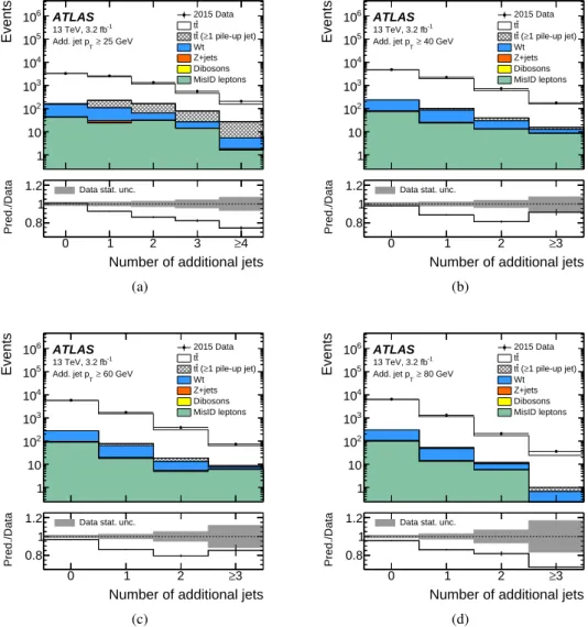
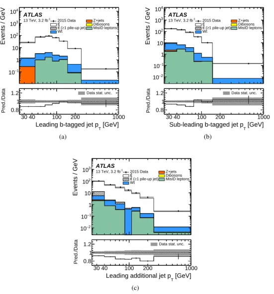
After the event selection, only about 4.5% of the events are background, as listed in Table1. The back-ground is dominated by single top production (3.1%) and fake leptons (1.6%). The event yields and the relative background contributions vary with jet multiplicity and jet pTas shown in Figures1and 2, respectively. The single-top background dominates across all jet pTvalues and at low additional jet mul-tiplicities. At high jet multiplicities (≥ 3 additional jets) the fake-lepton background exceeds the number of single-top events. While the number of events observed in the 0-jet bin agrees with the prediction within the uncertainties, the data exceed the predictions increasingly with jet multiplicity, reaching a 25% deviation for events with at least four additional jets above 25 GeV.

The table and figures also list the contribution of t¯t events with at least one additional jet identified as originating from pile-up (pile-up jets). These are signal events, but a few pile-up jets are still in the sample after object and event selection, as the background suppression of the JVT cut is very high but not 100%. Due to the presence of at least one jet that does not originate from the hard interaction, these events may appear in the wrong jet multiplicity bin. In the jet pT spectra, pile-up jets contribute at low additional-jet pT as the pile-up jets are generally softer than the jets in t¯t events. For the same reason, pile-up jets only contribute significantly to the jet multiplicity distributions with the 25 GeV threshold. In most of the events with remaining pile-up jets, only one of the additional jets is caused by pile-up. Any remaining pile-up jets can be identified in the simulation, but not in data. Therefore the data are corrected for pile-up jets in the unfolding procedure, as described later.

Process Yield

Single top (Wt) 236 ±2 (stat.) ±46 (syst.) Fake leptons 117 ±22 (stat.) ±120 (syst.)

Z+jets 6 ±3 (stat.) ±1 (syst.)

Dibosons 3.1 ±0.4 (stat.) ±1.5 (syst.) Total background 362 ±22 (stat.) ±130 (syst.) tt(≥ 1 pile-up jet 310 ±2 (stat.) ±88 (syst.) tt(no pile-up jets) 6850 ±11 (stat.) ±940 (syst.) Expected 7520 ±25 (stat.) ±950 (syst.)

Observed 8050

Events 1 10 2 10 3 10 4 10 5 10 6 10 2015 Data t t 1 pile-up jet) ≥ ( t t Wt Z+jets Dibosons MisID leptons ATLAS -1 13 TeV, 3.2 fb 25 GeV ≥ T Add. jet p

Number of additional jets

0 1 2 3 ≥4

Pred./Data 0.8

1

1.2 Data stat. unc.

(a) Events 1 10 2 10 3 10 4 10 5 10 6 10 2015 Data t t 1 pile-up jet) ≥ ( t t Wt Z+jets Dibosons MisID leptons ATLAS -1 13 TeV, 3.2 fb 40 GeV ≥ T Add. jet p

Number of additional jets

0 1 2 ≥3

Pred./Data 0.8

1

1.2 Data stat. unc.

(b) Events 1 10 2 10 3 10 4 10 5 10 6 10 2015 Data t t 1 pile-up jet) ≥ ( t t Wt Z+jets Dibosons MisID leptons ATLAS -1 13 TeV, 3.2 fb 60 GeV ≥ T Add. jet p

Number of additional jets

0 1 2 ≥3

Pred./Data 0.8

1

1.2 Data stat. unc.

(c) Events 1 10 2 10 3 10 4 10 5 10 6 10 2015 Data t t 1 pile-up jet) ≥ ( t t Wt Z+jets Dibosons MisID leptons ATLAS -1 13 TeV, 3.2 fb 80 GeV ≥ T Add. jet p

Number of additional jets

0 1 2 ≥3

Pred./Data 0.8

1

1.2 Data stat. unc.

(d)

Figure 1: Multiplicity of additional jets with (a) pT> 25 GeV, (b) pT> 40 GeV, (c) pT> 60 GeV, and (d) pT> 80 GeV

for selected events at reconstruction level in data and simulation. Simulated signal events with at least one additional jet identified as pile-up are indicated in grey. The contribution of pile-up jets to the backgrounds is negligible. The lower panel shows the ratio of the total prediction to the data (solid line), the grey band represents the statistical uncertainty of the measurement, and the error bars on the solid line show the statistical uncertainty in the signal MC sample.

Events / GeV 1 − 10 1 10 2 10 3 10 4 10 2015 Data Z+jets t t Dibosons 1 pile-up jet) ≥ ( t t MisID leptons Wt ATLAS -1 13 TeV, 3.2 fb [GeV] T

Leading b-tagged jet p

30 40 100 200 1000

Pred./Data 0.8 1

1.2 Data stat. unc.

(a) Events / GeV 2 − 10 1 − 10 1 10 2 10 3 10 4 10 2015 Data Z+jets t t Dibosons 1 pile-up jet) ≥ ( t t MisID leptons Wt ATLAS -1 13 TeV, 3.2 fb [GeV] T

Sub-leading b-tagged jet p

30 40 100 200 1000

Pred./Data 0.8 1

1.2 Data stat. unc.

(b) Events / GeV 2 − 10 1 − 10 1 10 2 10 3 10 2015 Data Z+jets t t Dibosons 1 pile-up jet) ≥ ( t t MisID leptons Wt ATLAS -1 13 TeV, 3.2 fb [GeV] T

Leading additional jet p

30 40 100 200 1000

Pred./Data 0.8

1

1.2 Data stat. unc.

(c)

Figure 2: (a) Leading b-tagged jet pT, (b) sub-leading b-tagged jet pT, and (c) leading additional-jet pTfor selected

events at reconstruction level. The last bin includes overflows. Jets identified as pile-up in the t¯t signal sample are indicated in grey. The contribution of pile-up jets to the backgrounds is negligible. The lower panel shows the ratio of the total prediction to the data (solid line), the grey band represents the statistical uncertainty of the measurement, and the error bars on the solid line shows the statistical uncertainty in the signal MC sample.

6 Sources of systematic uncertainty

The systematic uncertainties of the reconstructed objects, in the signal modelling and in the background estimates, are evaluated as described in the following.

The jet energy scale (JES) uncertainty is evaluated by varying 19 uncertainty parameters derived from in situ analyses at √s = 8 TeV and extrapolated to data at √s = 13 TeV [51]. The JES uncertainty is 5.5% for jets with pT of 25 GeV and quickly decreases with increasing jet pT, falling to below 2% for jets above 80 GeV. The uncertainty in the jet energy resolution (JER) is calculated by extrapolating the uncertainties derived at √s= 8 TeV to √s = 13 TeV [51]. The uncertainty in JER is at most 3.5% at pT of 25 GeV, quickly decreasing with increasing jet pTto below 2% for jets above 50 GeV.

Uncertainties on the efficiency for tagging b-jets were determined using the methods described in Ref. [52] applied to dileptonic ttbar events in √s = 13 TeV data. The uncertainties on mistagging of charm and light jets were determined using √s = 8 TeV data as described in Refs. [53] and [54]. Additional uncertainties are assigned to take into account the presence of the new IBL detector and the extrapolation to √s= 13 TeV [50].

The lepton-related uncertainties are assessed mostly using Z → µ+µ−and Z → e+e−decays measured in √

s= 13 TeV data. The differences between the topologies of Z and t¯tpair production events are expected not to be significant for the estimation of uncertainties.

The uncertainty associated with the amount of QCD initial- and final-state radiation is evaluated as the dif-ference between the baseline MC sample and the corresponding RadHi and RadLo samples described in Section3. The uncertainty due to the choice of parton-shower and hadronisation algorithms in the signal modelling is assessed by comparing the baseline MC sample (Powheg+Pythia6) with Powheg+Herwig++. The uncertainty due to the use of a specific NLO MC sample with its particular matching algorithm is derived from the comparison of Powheg+Herwig++ to the MG5_aMC@NLO+Herwig++ sample. The uncertainty due to the particular PDF used for the signal model prediction is evaluated by taking the standard deviation of variations from 100 eigenvectors of the recommended Run-2 PDF4LHC [55] set and adding them in quadrature with the difference between the central predictions from CT10 and CT14 [56].

The uncertainty in the single top-quark background is evaluated based on the 5.3% error in the approx-imate NNLO cross-section prediction and by comparing samples with diagram removal and diagram subtraction schemes, as described in Section3. The uncertainty in the background from fake leptons is estimated to be 100% from the statistical uncertainty of the same-sign event counts in data and an interpol-ation error using the envelope of the differences of individual subcomponents (such as photon-conversion, heavy-flavour decay leptons, for example) of misidentified lepton background between the same-sign and the opposite-sign sample.

For Z+jets backgrounds, the scale factor derived in the e+_e−_{and µ}+_µ−_{channels and used to reweight the} signal-region distribution is varied by 22%, corresponding to the difference in the scale factors derived in subsamples with and without an additional jet. This value covers the variations of the correction factor derived from subsets of events with different jet multiplicities. No theoretical uncertainty is applied to the Z+jets background normalisation as this is scaled to data.

The uncertainty in the amount of pile-up is estimated by changing the nominal MC reweighting factors to vary the number of interactions per bunch crossing in data up and down by 10%. Two methods were

used to estimate the amount of interactions per bunch crossing. The first method calculated the number of interactions using the instantaneous luminosity and the inelastic proton-proton cross section [57,58]. The results of the calculation were compared to results from a data-driven method based on the number of reconstructed vertices. The difference between the correlation of the two methods in data and MC is taken as the uncertainty.

The uncertainty due to the 2–3% loss of hard-scatter jets due to the JVT cut is estimated using Z+jet events. The uncertainty in the efficiency of the JVT cut to reduce pile-up jets is estimated by using a sideband method. The JVT cut is inverted in simulation to estimate the number of pile-up jets and derive a scale factor to describe the number of pile-up jets in data. This factor is then used to scale the predicted number of pile-up jets in the signal region (with the JVT cut applied). Scale factors are also derived using the samples with increased and decreased pile-up mentioned above, and the larger of two variations is taken as systematics.

7 Definition of the fiducial phase space

For the measurement of the jet multiplicity, the jet pTspectra and the gap fractions, the data are corrected to particle level by comparing to events from MC generators in the fiducial volume described below. The fiducial volume, i.e., the object definitions and the kinematic phase space at particle level, is designed to match the reconstruction level as closely as possible and follow closely the definitions in Refs. [4,

5]. Leptons and jets are defined using particles with a mean lifetime greater than 0.3 × 10−10s, directly produced in pp interactions or from subsequent decays of particles with a shorter lifetime. Leptons from W boson decays (e, µ, νe, νµ, ντ) are identified as such by requiring that they are not hadron decay products. Electron and muon four-momenta are calculated after the addition of photon four-momenta within a cone of∆R = 0.1 around their original directions.

Jets are defined using the anti-kt algorithm with a radius parameter of 0.4. All particles are considered for jet clustering, except for leptons from W decays as defined above (i.e., neutrinos from hadron decays are included in jets) and any photons associated with the selected electrons or muons. Jets initiated by b-quarks are identified as such, i.e., identified as b-jets if a hadron with pT> 5 GeV containing a b-quark is associated with the jet through a ghost-matching technique as described in Ref. [59].

The cross-section is defined using events with exactly one electron and one muon with opposite-sign directly from W boson decays, i.e. excluding electrons and muons from decay of the τ leptons. In addition, at least two b-jets each with pT> 25 GeV and |η| < 2.5 are required. Following the reconstructed object selection, events with jet–electron pairs or jet–muon pairs with∆R < 0.4 are excluded. Additional jets are considered within |η| < 2.5 for pTthresholds of 25 GeV or higher, independently of their flavour.

8 Measurement of jet multiplicities and p

spectra

The multiplicities of additional reconstructed jets with different pT thresholds are corrected to particle level within the fiducial volume as defined above. Even though the kinematic range of the measurement is chosen to be the same for particle-level and reconstruction-level objects, corrections are necessary due to the efficiencies and detector resolutions that cause differences between reconstruction-level and

particle-level jet distributions. Examples include events in which one or more particle-level jets do not pass the pTthreshold for reconstruction-level jets and when the selection efficiency for inclusive t¯tevents changes as a function of jet multiplicity. Furthermore, additional reconstructed jets without a correspond-ing particle-level jet may appear due to pile-up, or if a jet migrates into the fiducial volume due to an upward fluctuation caused by the pT resolution, or if a single particle-level jet is reconstructed as two separate jets. These effects lead to migrations between bins and are taken into account within an iterative Bayesian unfolding [60].

The reconstructed jet multiplicity measurements are corrected separately for each additional-jet pTthreshold according to

N_unfoldi = 1 f_ei_ff ·

X j

(M−1)part,i_{reco, j}· f_acceptj (N_dataj − N_bgj ), (1) where N_unfoldi is the total number of fully corrected particle-level events with particle-level jet multiplicity i. The term f_effi represents the efficiency to reconstruct an event with i additional jets, defined as the ratio of events with i particle-level jets that fulfil both the fiducial volume selection at particle-level and the reconstruction-level selection, N_reco∧parti , to the number of events that fulfil the particle-level selection, N_parti :

f_ei_ff =

N_reco∧parti

N_parti . (2)

The resulting ratio f_ei_ff is approximately 0.33 and has very small dependence on the jet multiplicity. The analysis of different t¯t MC samples results in values of fi

eff which vary by up to 10%. The variations of f_ei_ff between different pT thresholds are less than 2%. The function f

j

accept is the probability of an event fulfilling the reconstruction-level selection and with j reconstructed jets, Nrecoj , to also be within the particle-level acceptance defined in Section7:

f_acceptj =

N_reco∧partj

N_recoj

. (3)

The variable N_dataj is the number of events in data with j reconstructed jets and N_bgj is the number of background events, as evaluated in Section5. The resulting f_acceptj decreases from around 0.85 for events without additional jets to about 0.76 for the highest jet multiplicities. The MC predictions of f_acceptj agree within 1% for events without any additional jets and within 5% at high jet multiplicities. Only MG5_aMC@NLO+Herwig++ predicts a smaller change as a function of the number of jets.

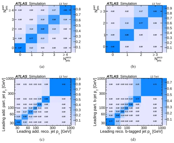
The response matrix M_{reco, j}part,i represents the probability P(Nrecoj |Nparti ) of finding an event with true particle-level jet multiplicity i with a reconstructed jet multiplicity j. As shown in Figure3, at the higher jet pT thresholds, at least 77% of the events have the same jet multiplicity at particle level and at reconstruction level. At the 25 GeV threshold, the agreement still exceeds 64%. The worse agreement can be explained in part by the presence of pile-up jets, which leads to events with more reconstructed than particle-level jets. There are almost no events with a difference of more than one jet between particle and reconstruction-level multiplicity.

As part of the Bayesian unfolding using Equation (1), Mpart,i_{reco, j}is calculated iteratively, i.e., the result of the first iteration is used as the reconstruction-level jet multiplicity for the following one. The corrected spectra are found to converge after four iterations of the Bayesian unfolding algorithm.

The unfolded additional-jet multiplicity distributions are normalised after the last iteration according to 1 σ dσ dNi = N_unfoldi P iN_unfoldi , (4) where Ni

unfold, as defined in Equation (1), corresponds to the number of events with i jets after full unfold-ing and σ is the measured t¯t production cross section in the fiducial volume.

A potential bias of the unfolded results due to data statistics and the unfolding procedure is investigated using pseudo-experiments by performing Gaussian sampling of the reconstruction-level distributions with statistical power equivalent to that present in data. The size of the bias, defined as the relative difference between the unfolded and predicted particle-level distributions, is found to be within the statistical uncer-tainty of the data. To check the size of a potential bias of the unfolding due to the relation between recon-structed and particle level distributions, the particle-level distributions are reweighted to alternative MC samples. Pseudo-experiments are performed based on the resulting alternative spectrum at reconstruction level. The pseudo-experiments are unfolded using the original correction procedure. The relative dif-ference between the unfolded particle-level distribution and the predicted particle-level distribution from the alternative MC sample is found to be well within the modelling uncertainty. In addition, it is ensured that differences between the nominal and alternative particle-level distributions are at least as large as the difference between data and the predicted reconstruction-level distributions.

The effect of the uncertainties listed in Section6on the unfolded multiplicity and jet spectra is evaluated as follows. The uncertainties due to detector-related effects, such as JES, JER and b-tagging and data statistics, are propagated through the unfolding by varying the reconstructed objects for each uncertainty component by ±1σ. The modified spectrum is then used as N_dataj in Equation (1) for the iterative unfolding and the difference on the particle-level distribution is taken as the systematic uncertainty.

The uncertainties due to the MC modelling of the QCD initial- and final-state radiation (ISR/FSR) and the parton-shower uncertainty are evaluated by replacing the data with the corresponding alternative MC sample and using the response matrix and the correction factors from the baseline t¯t MC sample for unfolding. The result is compared to the particle-level distribution of the alternative MC sample and the difference is taken as a systematic uncertainty. The uncertainties due to the MC modelling of the NLO matrix element and the matching algorithm are estimated in a similar way by replacing the data with the MG5_aMC@NLO+Herwig++ sample but using the response matrix and correction factors from Powheg+Herwig++. The resulting uncertainties are symmetrised for each component.

To unfold the leading and sub-leading b-jet pTand the leading additional-jet pT, the same ansatz is used as for the jet multiplicity measurement, but with the jet pTinstead of the jet multiplicity in the matrix, the acceptance and the efficiency formula. The binning is chosen to limit the migration, such that most events have reconstruction-level jet pTin the same region as the particle-level jet pT, and to limit the uncertainty due to data statistics. The efficiency correction f_ei_ff for the b-jets has a significant pT dependence: it is around 0.2 for the lowest pTbin and reaches approximately 0.35 at pTof 80 GeV. The efficiency for the additional jet varies only slightly between 0.28 and 0.31. The acceptance correction is between 0.8 and 0.9 for all jets and almost independent of pT, except at very low pT, at which it decreases significantly, to 0.56 for the leading additional jet. The unfolding response matrix presented in Figure3shows that more than 60% of the jets are in the same pTbin at particle and reconstruction level.

0.1 0.2 0.3 0.4 0.5 0.6 0.7 0.8 0.87 0.12 0.01 0.00 0.00 0.08 0.77 0.13 0.01 0.00 0.01 0.14 0.69 0.14 0.02 0.00 0.02 0.19 0.64 0.16 0.00 0.00 0.02 0.17 0.81 reco jets N 0 1 2 3 ≥ 4 part jets N 0 1 2 3 4 ≥

ATLAS Simulation 13 TeV

(a) 0.1 0.2 0.3 0.4 0.5 0.6 0.7 0.8 0.9 0.96 0.04 0.00 0.00 0.09 0.86 0.05 0.00 0.01 0.16 0.77 0.06 0.00 0.02 0.17 0.81 reco jets N 0 1 2 ≥ 3 part jets N 0 1 2 3 ≥

ATLAS Simulation 13 TeV

(b) 0.1 0.2 0.3 0.4 0.5 0.6 0.7 0.8 0.9 0.83 0.16 0.01 0.00 0.00 0.00 0.00 0.18 0.69 0.12 0.00 0.00 0.00 0.00 0.01 0.17 0.72 0.10 0.01 0.00 0.00 0.01 0.01 0.18 0.68 0.11 0.01 0.00 0.01 0.01 0.01 0.13 0.76 0.08 0.00 0.00 0.01 0.01 0.01 0.08 0.86 0.03 0.00 0.01 0.01 0.01 0.01 0.06 0.91 [GeV] T

Leading add. reco. jet p

2

10 ₁₀3

[GeV] _T

Leading add. part. jet p

2

10

3

10 ATLAS Simulation 13 TeV

30 60 100 300 1000 30 60 100 300 1000 (c) 0.1 0.2 0.3 0.4 0.5 0.6 0.7 0.77 0.22 0.00 0.00 0.00 0.00 0.00 0.16 0.69 0.14 0.00 0.00 0.00 0.00 0.03 0.24 0.62 0.11 0.00 0.00 0.00 0.01 0.06 0.24 0.61 0.08 0.00 0.00 0.00 0.02 0.05 0.22 0.66 0.05 0.00 0.00 0.00 0.01 0.04 0.20 0.73 0.01 0.00 0.00 0.00 0.01 0.02 0.25 0.71 [GeV] T

Leading reco. b-tagged jet p

2

10 ₁₀3

[GeV] _T

Leading part. b-jet p

2

10

3

10 ATLAS Simulation 13 TeV

30 60 100 300 1000 30 60 100 300 1000 (d)

Figure 3: Unfolding response matrices to match distributions (jet multiplicity, jet pT) at reconstruction level to

particle-level distributions in the fiducial phase space. Only events that fulfil the reconstruction- (particle-) level selection are included. Matrices to unfold (a) jet multiplicity for additional jets with pT> 25 GeV, (b) jet multiplicity

for additional jets with pT> 40 GeV, (c) jet pTof the leading additional jet, and (d) jet pTof the leading b-jet.

1 σ dσ dpi_T = Ni_p T,unfold ∆pi T P iNi_p T,unfold , (5) where Ni_p

T,unfold, as defined in Equation (1), corresponds to the number of events with the jet pTin bin i after full unfolding.

The measurement of the jet pTspectra is as stable as the jet multiplicity measurements and the biases are small.

8.1 Jet multiplicity results

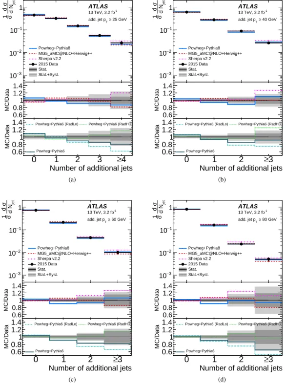
The unfolded normalised cross-sections are shown in Figure4and are compared to different MC

pre-dictions. Events with up to three additional jets with pT above 25 GeV are measured exclusively (four jets inclusively) and up to two additional jets exclusively (three inclusively) for the higher pTthresholds. Tables2to5list the detailed composition of the uncertainties for 25 GeV to 80 GeV. The jet multiplicity distributions are measured with an uncertainty of 4–5% for one additional jet, about 10% for two addi-tional jets, and around 20% for the highest jet multiplicity bin, except for the 80 GeV threshold where the

statistical uncertainty is larger for higher jet multiplicity bins. Systematic uncertainties dominate in all the measurements. In almost all bins for all pT thresholds, the JES uncertainty dominates, followed by the modelling uncertainty.

The data are compared to Powheg and MG5_aMC@NLO matched with different shower generators, namely Pythia8, Herwig++, and Herwig7 and to Sherpa, as shown in Figures4and5. Most predictions are within uncertainties and only slight deviations are visible except for Powheg+Herwig7, which deviates significantly from the data for all pTthresholds. The MG5_aMC@NLO predictions agree within 5–10% regardless of which parton shower is used (except Herwig7), and the Powheg predictions vary slightly more. The variations are larger when using different matrix elements but the same parton shower. The unfolded data are compared with different MC predictions using χ2_{tests. Full covariance matrices} are produced from the unfolding taking into account statistical and all systematic uncertainties. The cor-relation of the measurement bins is similar for all jet pTthresholds: strong anti-correlations exist between events with no additional jet and events with any number of additional jets. Positive correlations exist between the bins with one and two additional jets. The χ2is determined using:

χ2_{= S}T n−1Cov

−1

n−1Sn−1 (6)

where Sn−1 is a column vector representing the difference between the unfolded data and the MC gen-erator predictions of the normalised cross-section for one less than the total number of bins in the distri-bution, and Covn−1 is a matrix with n − 1 rows and the respective n − 1 columns of the full covariance matrix. The full covariance matrix is singular and non-invertible, as it is evaluated using normalised dis-tributions. The p-values are determined using the χ2and n − 1 degrees of freedom. Table9shows the χ2 and p-values.

A statistical comparison taking into account the bin correlations indicates that the agreement with data is slightly better for MG5_aMC@NLO+Herwig++, as shown in Table9. The ratio of the data to predictions of Powheg+Pythia6 with different levels of QCD radiation both in the matrix-element calculation and in the parton shower is also shown. Powheg+Pythia6 (RadLo) does not describe the data well. The central prediction of Powheg+Pythia6 yields fewer jets than in data; however, the predictions are still within the experimental uncertainties. Powheg+Pythia6 (RadHi) describes the data most consistently, which is also confirmed by high p-values for all pT thresholds. The Powheg+Pythia6 (RadLo) sample has p-values around 0.5 and the central sample mostly between 0.8 and 0.9.

8.2 Jet pTspectra results

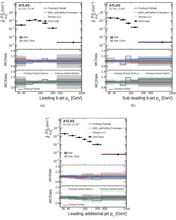
The particle-level normalised cross-sections differential in jet pTare shown in Figure6and are compared to different MC predictions. The total uncertainty in the pT measurements is 5–11%, although higher at some edges of the phase space. The uncertainty is dominated by the statistical uncertainty in almost all bins. The systematic uncertainties are listed in Tables6 to 8. JES/JER, NLO generator modelling

and PS/hadronisation are all significant and one of them is always the dominant source of systematic uncertainty. JES/JER is the main source of uncertainty in the lowest pTbins of all measurements. The predictions agree with data for all jet pT distributions as shown in Figure6and Figure7, although the predictions of Powheg+Herwig++ and MG5_aMC@NLO+Pythia8 do not give a good description of the leading additional-jet pT distribution, which is consistent with the jet multiplicity results. This is reflected by the statistical comparison as well (Table10).

Number of additional jets 0 1 2 3 ≥4 jet d N σ d σ 1 3 − 10 2 − 10 1 − 10 1 ATLAS -1 13 TeV, 3.2 fb 25 GeV ≥ T add. jet p Powheg+Pythia8 MG5_aMC@NLO+Herwig++ Sherpa v2.2 2015 Data Stat. Stat.+Syst.

Number of additional jets

0 1 2 3 ≥4 MC/Data 0.6 0.8 1 1.2 1.4

Number of additional jets

0 1 2 3 ≥4 MC/Data 0.6 0.8 1 1.2

1.4 Powheg+Pythia6 (RadLo) Powheg+Pythia6 (RadHi) Powheg+Pythia6

(a)

Number of additional jets

0 1 2 ≥3 jet d N σ d σ 1 3 − 10 2 − 10 1 − 10 1 ATLAS -1 13 TeV, 3.2 fb 40 GeV ≥ T add. jet p Powheg+Pythia8 MG5_aMC@NLO+Herwig++ Sherpa v2.2 2015 Data Stat. Stat.+Syst.

Number of additional jets

0 1 2 ≥3 MC/Data 0.6 0.8 1 1.2 1.4

Number of additional jets

0 1 2 ≥3 MC/Data 0.6 0.8 1 1.2

1.4 Powheg+Pythia6 (RadLo) Powheg+Pythia6 (RadHi) Powheg+Pythia6

(b)

Number of additional jets

0 1 2 ≥3 jet d N σ d σ 1 3 − 10 2 − 10 1 − 10 1 ATLAS -1 13 TeV, 3.2 fb 60 GeV ≥ T add. jet p Powheg+Pythia8 MG5_aMC@NLO+Herwig++ Sherpa v2.2 2015 Data Stat. Stat.+Syst.

Number of additional jets

0 1 2 ≥3 MC/Data 0.6 0.8 1 1.2 1.4

Number of additional jets

0 1 2 ≥3 MC/Data 0.6 0.8 1 1.2

1.4 Powheg+Pythia6 (RadLo) Powheg+Pythia6 (RadHi) Powheg+Pythia6

(c)

Number of additional jets

0 1 2 ≥3 jet d N σ d σ 1 3 − 10 2 − 10 1 − 10 1 ATLAS -1 13 TeV, 3.2 fb 80 GeV ≥ T add. jet p Powheg+Pythia8 MG5_aMC@NLO+Herwig++ Sherpa v2.2 2015 Data Stat. Stat.+Syst.

Number of additional jets

0 1 2 ≥3 MC/Data 0.6 0.8 1 1.2 1.4

Number of additional jets

0 1 2 ≥3 MC/Data 0.6 0.8 1 1.2

1.4 Powheg+Pythia6 (RadLo) Powheg+Pythia6 (RadHi) Powheg+Pythia6

(d)

Figure 4: Unfolded jet multiplicity distribution for different pTthresholds of the additional jets, for (a) additional

jet pT> 25 GeV, (b) additional jet pT> 40 GeV, (c) additional jet pT> 60 GeV, and (d) additional jet pT> 80 GeV.

Comparison to different MC predictions is shown for these distribution in first panel. The middle and bottom panels show the ratios of different MC predictions of the normalised cross-section to the measurement and the ratios of Powheg+Pythia6 predictions with variation of the QCD radiation to the measurement, respectively. The shaded regions show the statistical uncertainty (dark grey) and total uncertainty (light grey).

Relative uncertainty in [%] in additional jets multiplicity Sources 0 1 2 3 ≥ 4 Data statistics 2.1 2.7 4.0 6.0 9.0 JES/JER 5.0 1.8 7.0 12.0 16.0 b-tagging 0.5 0.2 0.7 1.4 2.0 ISR/FSR modelling 0.4 0.5 2.2 3.8 6.0 Signal modelling 1.9 2.0 5.6 6.0 11.0 Other 1.4 0.9 2.5 3.3 5.0 Total 6.0 4.0 10.0 16.0 24.0

Table 2: Summary of relative uncertainties in [%] for the jet multiplicity measurement using a jet pTthreshold of

25 GeV. "Signal modelling" sources of systematic uncertainty includes the hadronisation, parton shower and NLO modelling uncertainties. "Other" sources of systematic uncertainty refers to lepton and jet selection efficiencies, background (including pile-up jets) estimations, and the PDF.

Relative uncertainty in [%] in additional jets multiplicity

Sources 0 1 2 ≥ 3 Data statistics 1.7 2.7 5.0 9.0 JES/JER 2.0 2.5 6.0 9.0 b-tagging 0.3 0.4 1.1 1.8 ISR/FSR modelling 0.2 0.4 3.0 6.0 Signal modelling 2.0 3.7 4.4 9.0 Other 0.7 0.8 1.5 4.1 Total 3.4 5.0 10.0 17.0

Table 3: Summary of relative uncertainties in [%] for the jet multiplicity measurement using a jet pTthreshold of

40 GeV. "Signal modelling" sources of systematic uncertainty includes the hadronisation, parton shower and NLO modelling uncertainties. "Other" sources of systematic uncertainty refer to lepton and jet selection efficiencies, background (including pile-up jets) estimations, and the PDF.

Relative uncertainty in [%] in additional jets multiplicity

Sources 0 1 2 ≥ 3 Data statistics 1.5 3.0 7.0 15.0 JES/JER 0.9 2.3 4.2 7.0 b-tagging 0.2 0.6 1.2 2.0 ISR/FSR modelling 0.2 1.2 2.2 1.1 Signal modelling 0.7 1.6 5.0 9.0 Other 0.8 0.8 3.2 10.0 Total 2.0 4.4 10.0 22.0

Table 4: Summary of relative uncertainties in [%] for the jet multiplicity measurement using a jet pTthreshold of

60 GeV. "Signal modelling" sources of systematic uncertainty includes the hadronisation, parton shower and NLO modelling uncertainties. "Other" sources of systematic uncertainty refer to lepton and jet selection efficiencies, background (including pile-up jets) estimations, and the PDF.

Relative uncertainty in [%] in additional jets multiplicity Sources 0 1 2 ≥ 3 Data statistics 1.4 3.3 10.0 19.0 JES/JER 0.4 1.8 5.0 6.0 b-tagging 0.1 0.6 1.4 2.4 ISR/FSR modelling 0.1 1.3 6.0 4.5 Signal modelling 0.2 0.6 10.0 31.0 Other 0.8 1.4 3.1 6.0 Total 1.7 4.3 17.0 37.0

Table 5: Summary of relative uncertainties in [%] for the jet multiplicity measurement using a jet pTthreshold of

80 GeV. "Signal modelling" sources of systematic uncertainty includes the hadronisation, parton shower and NLO modelling uncertainties. "Other" sources of systematic uncertainty refer to lepton and jet selection efficiencies, background (including pile-up jets) estimations, and the PDF.

Relative uncertainty in leading b-jet pT[GeV] in [%]

Sources 25–45 45–65 65–85 85–110 110–150 150–250 > 250 Data statistics 11.0 5.0 4.3 4.2 4.4 5.0 12.0 JES/JER 11.0 2.3 1.3 2.4 3.2 4.2 6.0 b-tagging 6.0 1.1 0.9 1.0 1.9 5.0 14.0 ISR/FSR modelling 6.0 0.9 1.0 2.1 3.1 0.9 0.1 Signal modelling 9.0 2.0 5.0 6.0 2.1 0.4 15.0 Other 4.4 3.0 1.4 1.7 3.0 2.2 10.0 Total 20.0 7.0 7.0 8.0 8.0 8.0 26.0

Table 6: Summary of relative measurement uncertainties in [%] for the leading b-jet pT distribution. "Signal

modelling" sources of systematic uncertainty includes the hadronisation, parton shower and NLO modelling un-certainties. "Other" sources of systematic uncertainty refers to lepton and jet selection efficiencies, background (including pile-up jets) estimations, and the PDF.

Relative uncertainty in sub-leading b-jet pT[GeV] in [%]

Sources 25–40 40–55 55–75 75–100 100–150 > 150 Data statistics 4.0 4.2 3.9 6.0 7.0 11.0 JES/JER 5.0 2.5 3.4 3.8 3.6 6.0 b-tagging 2.8 1.2 2.2 2.3 3.6 11.0 ISR/FSR modelling 0.3 2.7 1.2 1.3 3.2 0.3 Signal modelling 6.0 1.9 6.0 8.0 6.0 5.0 Other 1.4 1.8 1.9 3.4 3.1 3.9 Total 9.0 6.0 9.0 11.0 11.0 18.0

Table 7: Summary of relative measurement uncertainties in [%] for the sub-leading b-jet pT distribution. ¨Signal

modelling" sources of systematic uncertainty includes the hadronisation, parton shower and NLO modelling un-certainties. "Other" sources of systematic uncertainty refers to lepton and jet selection efficiencies, background (including pile-up jets) estimations, and the PDF.

Relative uncertainty in leading additional jet pT[GeV] in [%] Sources 25–40 40–60 60–85 85–110 110–150 150–250 > 250 Data statistics 3.8 6.0 6.0 8.0 8.0 6.0 8.0 JES/JER 2.9 3.3 2.1 2.7 3.8 3.8 4.2 b-tagging 0.3 0.2 0.6 0.4 0.6 0.4 1.3 ISR/FSR modelling 0.6 1.6 1.4 0.7 2.4 4.0 2.1 Signal modelling 2.5 4.0 3.6 10.0 8.0 8.0 4.0 Other 1.5 2.8 1.8 3.4 2.4 1.6 1.8 Total 6.0 8.0 8.0 13.0 12.0 11.0 11.0

Table 8: Summary of relative measurement uncertainties in [%] for the leading additional jet pTdistribution.

"Sig-nal modelling" sources of systematic uncertainty includes the hadronisation, parton shower and NLO modelling uncertainties. "Other" sources of systematic uncertainty refers to lepton and jet selection efficiencies, background (including pile-up jets) estimations, and the PDF.

pT> 25 GeV pT> 40 GeV pT> 60 GeV pT> 80 GeV Generator χ2_{/NDF p-value χ}2_{/NDF p-value χ}2_{/NDF p-value χ}2_{/NDF p-value}

Powheg+Pythia6 0.82/4 0.94 0.83/3 0.84 1.01/3 0.80 1.82/3 0.61 Powheg+Pythia8 0.43/4 0.98 0.90/3 0.83 0.64/3 0.89 1.09/3 0.78 Powheg+Herwig++ 0.51/4 0.97 0.88/3 0.83 1.46/3 0.69 2.58/3 0.46 Powheg+Herwig7 8.62/4 0.07 4.87/3 0.18 3.17/3 0.37 2.57/3 0.46 MG5_aMC@NLO+Pythia8 5.51/4 0.24 3.10/3 0.38 2.25/3 0.52 2.20/3 0.53 MG5_aMC@NLO+Herwig++ 1.28/4 0.86 0.49/3 0.92 0.34/3 0.95 0.40/3 0.94 MG5_aMC@NLO+Herwig7 3.14/4 0.54 4.31/3 0.23 3.57/3 0.31 2.87/3 0.41 Sherpa v2.2 0.43/4 0.98 0.85/3 0.84 0.74/3 0.86 0.79/3 0.85 Powheg+Pythia6 (RadHi) 1.20/4 0.88 1.06/3 0.79 0.22/3 0.97 0.22/3 0.97 Powheg+Pythia6 (RadLo) 4.15/4 0.39 2.05/3 0.56 2.08/3 0.56 2.87/3 0.41

Table 9: Values of χ2_{/NDF and p-values between the unfolded normalised cross-section and the predictions for}

additional-jet multiplicity measurements. The number of degrees of freedom is equal to the number of bins minus one.

Leading b-jet pT Sub-leading b-jet pT Leading additional jet pT Generator χ2_{/NDF p-value χ}2_{/NDF p-value χ}2_{/NDF p-value}

Powheg+Pythia6 2.24/6 0.90 5.85/5 0.32 3.50/6 0.74 Powheg+Pythia8 1.94/6 0.93 6.33/5 0.28 2.28/6 0.89 Powheg+Herwig++ 1.95/6 0.92 6.91/5 0.23 18.5/6 0.01 Powheg+Herwig7 1.26/6 0.97 5.44/5 0.36 1.95/6 0.92 MG5_aMC@NLO+Pythia8 1.99/6 0.92 6.76/5 0.24 10.5/6 0.10 MG5_aMC@NLO+Herwig++ 2.03/6 0.92 6.94/5 0.23 2.97/6 0.81 MG5_aMC@NLO+Herwig7 1.32/6 0.97 4.80/5 0.44 2.31/6 0.89 Sherpav2.2 0.71/6 0.99 5.37/5 0.37 4.03/6 0.67

Powheg+Pythia6 (RadHi) 2.79/6 0.83 6.55/5 0.26 1.68/6 0.95

Powheg+Pythia6 (RadLo) 2.16/6 0.90 5.55/5 0.35 3.27/6 0.77

Table 10: Values of χ2_{/NDF and p-values between the unfolded normalised cross-section and the predictions for}

the jet pTmeasurements. The number of degrees of freedom is equal to one less than the number of bins in the

Number of additional jets

0

1

2

3

≥

4

Number of additional jets

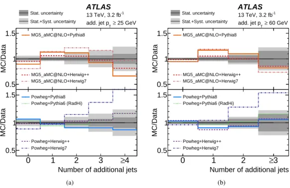
0 1 2 3 ≥4 MC/Data 0.5 1 1.5 Powheg+Pythia8 Powheg+Pythia6 (RadHi) Powheg+Herwig++ Powheg+Herwig7 (a)

Number of additional jets

0

1

2

≥

3

Number of additional jets

0 1 2 ≥3 MC/Data 0.5 1 1.5 Powheg+Pythia8 Powheg+Pythia6 (RadHi) Powheg+Herwig++ Powheg+Herwig7 (b)

Figure 5: Ratios of jet multiplicity distribution for different pTthresholds of the additional jets predicted by various

MC generators to the unfolded data, for (a) additional jet pT> 25 GeV, (b) additional jet pT> 60 GeV. The shaded

[GeV] T Leading b-jet p 2 10 103 ] -1 [GeV jet T d p σ d σ 1 5 − 10 4 − 10 3 − 10 2 − 10 1 − 10 1 Powheg+Pythia8 MG5_aMC@NLO+Herwig++ Sherpa v2.2 2015 Data ATLAS -1 13 TeV, 3.2 fb Stat. Stat.+Syst. [GeV] T Leading b-jet p 2

10

10

Powheg+Pythia6 (RadLo) Powheg+Pythia6 (RadHi)

Powheg+Pythia6 (a) [GeV] T Sub-leading b-jet p 2 10 103 ] -1 [GeV jet T d p σ d σ 1 5 − 10 4 − 10 3 − 10 2 − 10 1 − 10 1 Powheg+Pythia8 MG5_aMC@NLO+Herwig++ Sherpa v2.2 2015 Data ATLAS -1 13 TeV, 3.2 fb Stat. Stat.+Syst. [GeV] T Sub-leading b-jet p2

10

10

Powheg+Pythia6 (RadLo) Powheg+Pythia6 (RadHi)

Powheg+Pythia6

(b)

[GeV]

T

Leading additional jet p

2 10 103 ] -1 [GeV jet T d p σ d σ 1 5 − 10 4 − 10 3 − 10 2 − 10 1 − 10 1 Powheg+Pythia8 MG5_aMC@NLO+Herwig++ Sherpa v2.2 2015 Data ATLAS -1 13 TeV, 3.2 fb Stat. Stat.+Syst. [GeV] T

Leading additional jet p

10

10

MC/Data _0.8 1 1.2 1.4 [GeV] T Leading additional jet p

30 40 100 200 300 1000

MC/Data _0.8

1 1.2 1.4

Powheg+Pythia6 (RadLo) Powheg+Pythia6 (RadHi)

Powheg+Pythia6

(c)

Figure 6: Unfolded jet pT distribution for (a) leading b-jet, (b) sub-leading b-jet and (c) leading additional jet.

Comparison to different MC predictions is shown for these distribution in first panel. The middle and bottom panels show the ratios of different MC predictions of the normalised cross-section to the measurement and the ratios of Powheg+Pythia6 predictions with variation of the QCD radiation to the measurement, respectively. The shaded regions show the statistical uncertainty (dark grey) and total uncertainty (light grey).

[GeV] T Leading b-jet p 2 10 103 MC/Data 0.5 1 1.5 ATLAS -1 13 TeV, 3.2 fb Stat. uncertainty Stat.+Syst. uncertainty MG5_aMC@NLO+Pythia8 MG5_aMC@NLO+Herwig++ MG5_aMC@NLO+Herwig7 [GeV] T Leading b-jet p 30 40 100 200 1000 MC/Data 0.5 1 1.5 Powheg+Pythia8 Powheg+Pythia6 (RadHi) Powheg+Herwig++ Powheg+Herwig7 (a) [GeV] T Sub-leading b-jet p 2 10 103 MC/Data 0.5 1 1.5 ATLAS -1 13 TeV, 3.2 fb Stat. uncertainty Stat.+Syst. uncertainty MG5_aMC@NLO+Pythia8 MG5_aMC@NLO+Herwig++ MG5_aMC@NLO+Herwig7 [GeV] T Sub-leading b-jet p 30 40 100 200 1000 MC/Data 0.5 1 1.5 Powheg+Pythia8 Powheg+Pythia6 (RadHi) Powheg+Herwig++ Powheg+Herwig7 (b) [GeV] T Leading additional jet p

2 10 103 MC/Data 0.5 1 1.5 ATLAS -1 13 TeV, 3.2 fb Stat. uncertainty Stat.+Syst. uncertainty MG5_aMC@NLO+Pythia8 MG5_aMC@NLO+Herwig++ MG5_aMC@NLO+Herwig7 [GeV] T

Leading additional jet p

30 40 100 200 1000 MC/Data 0.5 1 1.5 Powheg+Pythia8 Powheg+Pythia6 (RadHi) Powheg+Herwig++ Powheg+Herwig7 (c)

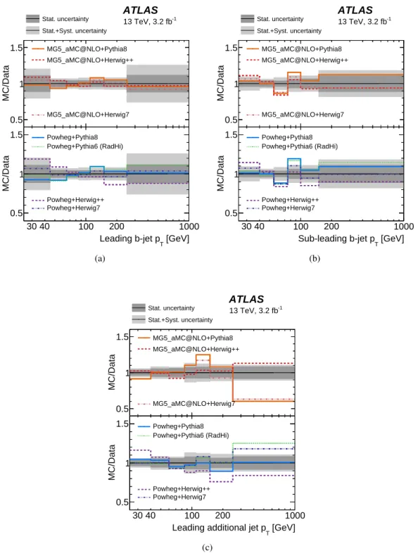
Figure 7: Ratios of jet pT distribution for (a) leading b-jet, (b) sub-leading b-jet and (c) leading additional jet

predicted by various MC generators to the unfolded data. The shaded regions show the statistical uncertainty (dark grey) and total uncertainty (light grey).

9 Gap fraction measurements

The jet activity is also studied by measuring the gap fraction fgap, defined as the fraction of events with no jet activity in addition to the two b-tagged jets above a given pTthreshold in a “veto region” defined as a rapidity region in the detector. The transverse momentum threshold is defined in two ways, and the gap fraction in two ways accordingly. First, the gap fraction is measured as the fraction of events without any additional jet in that rapidity region above a given pT threshold Q0:

fgap(Q0)= n(Q0)

N_tt , (7)

where Ntt is the total number of selected events, Q0is the pT threshold for any additional jet in the veto region of these events, and n(Q0) represents the subset of events with no additional jet with pT> Q0. The second type of gap fraction is defined as the fraction of events in which the scalar pT sum of all additional jets in the given veto region does not exceed a given threshold Qsum:

fgap(Qsum)=

n(Qsum)

N_tt . (8)

Here, n(Qsum) represents the subset of events in which the scalar pT sum of all additional jets in the veto region is less than Qsum. The gap fraction defined using Q0is mainly sensitive to the leading pTemission accompanying the t¯t system, whereas the gap fraction defined using Qsumis sensitive to all hard emissions accompanying the t¯t system. In the following descriptions of the gap fraction measurement process, the same procedure is followed for Qsumas for Q0.

Both types of gap fraction are measured in four veto regions: |y| < 0.8, 0.8 < |y| < 1.5, 1.5 < |y| < 2.1 and the full central region |y| < 2.1, where y is calculated as

y = 1 2ln E_{+ p}z E − pz ! . (9)

Furthermore, the gap fraction is measured considering jet activity in the full central region (|y| < 2.1) for four different subsamples specified by the mass of the eµ + 2 b-tagged jets system, meµbb. Both the rapidity region and the meµbbsubsamples are chosen to correspond to those used in earlier publications at lower energies [3,4].

The gap fraction f_gappart(Q0) (and analogously for fgappart(Qsum) in the following) is measured as defined in Equation (10) by counting the number of selected data events Ndataand the number ndata(Q0) of those that had no additional jets with pT > Q0within the veto region, where the sets of Q0and Qsumthreshold values correspond approximately to one standard deviation of the jet energy resolution and are the same as in the earlier publications [3,4]. The number of background events, Nbgand nbg(Q0), are then subtracted from these events:

fdata(Q0)=

ndata(Q0) − nbg(Q0) N_data− Nbg

(10) and similarly for fgappart(Qsum). The measured gap fraction fdata(Q0) is then corrected for detector effects to particle level by multiplying it by a correction factor C(Q0) to obtain fgappart(Q0). The correction factor C(Q0) is determined from the baseline Powheg+Pythia6 t¯tsample using the simulated gap fraction values at reconstruction level freco(Q0), and at particle level fpart(Q0) :

C(Q0)=

fpart(Q0) freco_(Q

0)

[GeV] 0 Q 50 100 150 200 250 300 Fractional Uncertainty 0.97 0.98 0.99 1 1.01 1.02 1.03 Total systematic ATLAS -1 =13 TeV, 3.2 fb s

Total Uncertainty Stat. Uncertainty (Data) JES/JER ISR/FSR Modelling PS/Hadronisation NLO Modelling b-tagging Other Sources

veto region: |y| < 0.8

Total systematic (a) [GeV] 0 Q 50 100 150 200 250 300 Fractional Uncertainty 0.94 0.96 0.98 1 1.02 1.04 1.06 Total systematic ATLAS -1 =13 TeV, 3.2 fb s

Total Uncertainty Stat. Uncertainty (Data) JES/JER ISR/FSR Modelling PS/Hadronisation NLO Modelling b-tagging Other Sources

veto region: |y| < 2.1

Total systematic

(b)

Figure 8: Envelope of fractional uncertainties ∆ f / f in the gap fraction fgappart(Q0), centred around unity, for (a)

|y| < 0.8 and (b) |y| < 2.1. The statistical uncertainty is shown by the shaded area, and the total uncertainty by the solid black line. The systematic uncertainty is shown broken down into several groups, each of which includes various individual components.

The values of the correction factors C(Q0) and C(Qsum) deviate by less than 4% from unity at low Q0 and Qsum values in the rapidity regions (less than 8% in the meµbb subsamples), and approach unity at higher threshold values. The small corrections reflect the high selection efficiency and high purity of the event samples. At each threshold Q0, the baseline simulation predicts that around 80% of the selected reconstructed events that do not have a jet with pT > Q0 also have no particle-level jet with pT > Q0. Therefore, a simple bin-by-bin correction method is considered adequate, rather than a full unfolding as used in Section8.

Systematic uncertainties arise in this procedure from the uncertainties in C(Q0) and the subtracted back-grounds. The uncertainties, as described in Section6, are used to recalculate fdata_(Q

0) and C(Q0) to obtain the gap fraction fgappart(Q0). The corresponding quantities for Qsumare calculated accordingly. Fig-ure8 and Table11 list the resulting relative uncertainty in f_gappart(Q0),∆ f / f , for the different sources of uncertainty in the full central rapidity region.

9.1 Gap fraction results in rapidity regions

Figure9 shows the measured gap fractions f_gappart(Q0) in data, corrected to the particle level. The gap fraction fgappart(Q0) is compared to various MC generator predictions in Figure10, and Figure11shows the measured gap fractions fgappart(Qsum) compared to various MC generators, corrected to the particle level. The predictions of Sherpa and MG5_aMC@NLO+Herwig++ agree well with each other and are within the uncertainties of the data, while Powheg+Pythia8 has slightly higher gap fractions, i.e., predicts too little radiation. Similarly to the jet multiplicity measurements, Powheg+Pythia6 (RadHi) agrees well with data, while the nominal and the Powheg+Pythia6 (RadLo) samples give similar but too high predictions compared to data. The results in Fig.9(d) can directly be compared with the jet multiplicity results in

Uncertainty in fgap(Q0) in [%] jet pTthreshold

25 45 65 95 110 150 250

Sources GeV GeV GeV GeV GeV GeV GeV

Data statistics 1.2 0.8 0.6 0.5 0.4 0.3 0.2 JES/JER 4.1 1.3 0.6 0.3 0.2 0.1 0.1 b-tagging 0.5 0.3 0.2 0.1 0.1 0.0 0.0 ISR/FSR modelling 0.4 0.0 0.1 0.1 0.1 0.0 0.0 Signal Modelling 4.5 1.4 1.0 0.7 0.3 0.4 0.1 Other 1.1 0.4 0.3 0.2 0.2 0.1 0.1 Total 6.3 2.1 1.3 0.9 0.6 0.6 0.2

Table 11: Sources of uncertainty in the gap fraction measurement as a function of Q0for the full central region

|y| < 2.1, for a selection of Q0 thresholds. "Signal modelling" sources of systematic uncertainty includes the

hadronisation, parton shower and NLO modelling uncertainties. "Other" sources of systematic uncertainty refer to lepton and jet selection efficiencies, background (including pile-up jets) estimations, and the PDF.

Fig.4and 5in the one additional jet bin. Here the Powheg+Pythia8 predictions are below data for all

distributions which proves the consistency of the measurements. The pTdistribution of the first additional jet shown in Fig.6contains only events with at least one additional jet and differs in this respect from the gap fraction distribution which includes events with no additional jet. However, the results are also consistent as Powheg+Pythia8 predicts a slightly softer pTspectrum for the additional jet which leads to the observed effect that less jets above the 25 GeV threshold are observed.

The matrix of statistical and systematic correlations is shown in Figure12for the gap fraction measure-ment at different values of Q0 for the full central |y| < 2.1 rapidity region. Nearby points in Q0 are highly correlated, while well-separated Q0 points are less correlated. The full covariance matrix, in-cluding correlations, is used to calculate a χ2value for the compatibility of each of the NLO generator predictions with the data in each veto region. The results are given in Tables12and13. An analysis of the p-values confirms that Powheg+Herwig++, MG5_aMC@NLO+Herwig7, MG5_aMC@NLO+Pythia8 and Powheg+Pythia6 (RadLo) are not consistent with the data. Powheg+Pythia6 (RadHi) has the best p-values among the QCD shower variations of Powheg+Pythia6.