Deorbiting and Reentry of GAMASAT

F

E

U

P

Deorbiting and Reentry of GAMASAT

Andrêa Corte-Real Albuquerque Costa

Mestrado Integrado em Engenharia Eletrotécnica e de Computadores Supervisor: PhD Sérgio Reis Cunha

c

Resumo

A importância do envio de satélites para o espaço e de todo o desenvolvimento que isso implica, vai para além do que a mente pode imaginar. Diariamente fazemos uso das suas vantagens, sem se quer ser evidente. Estudos de imagens para previsões meteorológicas ou com um simples toque num recetor GPS ter disponível em poucos segundos o melhor caminho até ao destino, são alguns dos exemplos do proveito dos satélites. Dessa forma, há uma forte crença no retorno que o investimento no processo de desenvolvimento de satélites pode trazer em setores como saúde, educação, ambiente e segurança; as suas aplicações estão em constante crescimento. Assim, como qualquer evolução é necessário pôr à prova equipamentos projectados, o que implica a necessidade de enviar equipamentos para o espaço e recuperá-los. Dessa forma, é cada vez mais crucial investir e encontrar formas rentáveis e seguras de controlar a perda de altitude de satélites e até mesmo a sua reentrada, ou pelo menos, algumas das suas subestruturas destes.

O principal foco desta tese, inserido no projeto GAMASAT, é ajudar a dar um passo nessa direção. Nela será descrito o processo de desenvolvimento para um sistema de controlo da perda de altitude sem ajuda de propulsores e assim recuperar informação recolhida no período de orbita do satélite.

O projeto GAMASAT resultou de uma parceria entre a Universidade do Porto e a TEKEVER, para projetar o lançamento de um CubeSat abrangido pela missão QB50. O satélite irá conter uma cápsula que procederá à reentrada, juntamente com outros subsistemas, nomeadamente sistemas de: comunicação, navegação, determinação de atitude e equipamentos para efeitos de estudos atmosféricos.

Este projeto será desenvolvido em ambiente MATLAB, com o propósito de estudar a perda de altitude do satélite e a estabilidade da cápsula durante a reentrada. Para o desenvolvimento do sistema de controlo foram necessários estudos preliminares do coeficiente de arrasto a que o satélite estará sujeito e os seus efeitos na atitude. Este satélite será um modelo CubeSat 3U, capaz de controlar a sua órbita com o ajuste da área exposta ao vento aparente, recorrendo uso de rodas de inércia . O algoritmo de controlo iniciará o processo de atuação nas rodas de acordo com a informação recolhida do receptor GPS, visando sempre o ajuste da trajetória de reentrada para uma aterragem segura. Num dos compartimento do CubeSat encontra-se a cápsula que fará a reentrada, contendo os seguintes equipamentos: Transmissor de rádio SDR, outro receptor GPS, baterias, sensores e um actuador passivo damping. Para uma maior segurança, a aterragem dar-se-à no mar, mais especificamente na Zona Económica Exclusiva de Portugal e para auxiliar a sua localização e recolha as comunicações serão realizadas por mensagens UHF ARGOS.

Abstract

The importance of sending satellites to space and the implied developments goes beyond what the mind can reach. In our day-to-day lives there are a number of examples of its applications, such as weather forecast studies or to find the best route, with the touch of your fingers in a GPS receiver. Therefore, there is a strong belief that investement in satellites can be even more helpful and produce a direct impact on health, education, environment and safety. New applications for satellites are continuously arising. Some involve retrieving material back from orbit. For that purpose, it is absolutely essential to find new cost-effective and safe ways to de-orbit and re-enter satellites or parts of satellites.

The main goal of this thesis is to take a step in that direction and to describe the development of the de-orbiting control system without propulsion, followed by the capsule re-entry to recover that information, which will be performed in a GAMASAT project.

The GAMASAT project is a partnership between the University of Porto and TEKEVER, to launch a CubeSat enrolled with QB50 mission. This satellite will contain a re-entry capsule, to-gether with other sub-systems: communications, navigation, attitude determination and equipment for atmospheric study.

This project will be developed in a MATLAB environment in order to study the satellite de-orbiting control and the re-entry capsule stability. In order to develop the control system for the de-orbiting, a drag coefficient study was primarily carried out, based on the satellite attitude. Being a 3U CubeSat, the de-orbiting control will be performed by reaction wheels that will change the exposed area to the ram direction. The control algorithm will cause actuation according to the navigation data from a GPS receiver and aims to adjust the re-entry trajectory towards reaching a safe landing area. The capsule that contains a SDR radio transmitter, another GPS receiver, batteries, sensors and a passive damping actuator will perform the re-entry. The landing will occur on the sea, more exactly on Exclusive Economic Zone of Portugal, and for its recovery the communication will be performed through UHF ARGOS messages for location determination.

Acknowledgments

I realized that I do not know where to begin. So, I just wanted to say that what I made it, I made it because all of you gave me the best of you guys. All of the pushes, the laughs and the supportive words did not made the things easier, but it made me not lose the forces. Thank you, thank you for the patience, thank you for the help, thank you for smiles, thank you be here or on the other side of the line. Writing your names here is just a small gesture that I found to show my appreciation for all of you have done, but was the way that I found to let you know that what you have done I will never forget. To all of you, Thank you:

António Côrte-Real

Kátia Miotelo

Mariana Santos

Margarida Carvalho

Nuno Sousa

Sérgio Reis Cunha

Susana Rafael

Tom Segert

"Human beings are divided into mind and body. The mind embraces all the nobler aspirations, like poetry and philosophy, but the body has all the fun."

Woody Allen

Contents

3 State of the Art 9 3.1 Overview . . . 9

3.2 Description of Existing Systems . . . 10

3.2.1 Inflatable Re-entry Demonstrator Technology - IRDT . . . 10

3.2.2 Inflatable Re-entry Vehicle Experiment - IRVE . . . 12

3.2.3 Hayabusa . . . 13

3.2.4 Young Engineers’ Satellite 2 - YES2 . . . 14

3.3 De-orbiting . . . 15

3.4 Re-entry . . . 15

4 De-orbiting Control 17 4.1 Atmosphere - Vertical Structure . . . 18

4.1.1 Density . . . 19

4.1.2 Temperature . . . 20

4.2 Drag Force vs attitude . . . 26

4.2.1 Drag Coefficient . . . 27

4.2.2 GAMASAT Drag Coefficient . . . 27

4.2.3 GAMASAT Drag Force . . . 32

4.3 Re-entry forecast . . . 32

4.3.1 Time of Control . . . 33

4.3.2 De-orbiting Control phase . . . 34

4.3.3 Control Strategy . . . 35

4.3.4 Release of Capsule . . . 36

4.4 Simulation . . . 36

x CONTENTS

4.4.1 Runge-Kutta method - Overview . . . 36

4.4.2 GAMASAT parameters . . . 37

4.4.3 Orbits Cycle . . . 40

4.4.4 Control Cycles . . . 40

4.4.5 Differential Drag . . . 41

4.4.6 Implementation in the capsule . . . 41

4.5 Simulation Results . . . 43

4.6 Conclusion . . . 49

5 Capsule Design 51 5.1 Introduction . . . 51

5.2 Design Requirements . . . 52

5.3 Reference Capsule Design . . . 52

5.4 Material Selection . . . 53

5.4.1 Cork Composite- P50 . . . 54

5.4.2 Carbon fibre-reinforced silicon carbide (C-SiC) . . . 54

5.4.3 Vacuum . . . 55 5.5 Capsule layout . . . 56 5.5.1 Floatability . . . 57 5.6 Final layout . . . 57 6 Re-entry Stability 61 6.1 Stabilization Method . . . 62

6.2 Calculation of Re-entry Stability . . . 63

6.2.1 Nyquist Analysis . . . 65

6.3 Capsule - Moment of Inertia . . . 66

6.3.1 Internal and External Inertia . . . 66

6.4 Simulation Results and Analysis . . . 67

6.5 Conclusion . . . 69

7 Future Work 71 7.1 De-orbiting . . . 71

7.2 Re-entry . . . 71

A GAMASAT Drag Coefficient 73

List of Figures

1.1 Work Plan . . . 2

2.1 Re-entry phases . . . 5

2.2 Distance variation with +/- 50% density variability . . . 6

3.1 a) IRDT; b) IRDT deployed . . . 11

3.2 a) IRVE deployment; b) IRDT deployed [6] . . . 13

3.3 a) Hayabusa release[8]; b) Hayabusa Replica [9] . . . 13

3.4 a) YES2 contains FLOYD , MASS and Fotino, the spherical re-entry capsule; b) YES2 assembled on FOTON-M spacecraft. [12] . . . 14

4.1 Drag force effect on the trajectory. Lower drag force overshoot the landing (black). Higher drag force, faster de-orbiting (red) . . . 17

4.2 Atmosphere Vertical structure . . . 18

4.3 Pressure vs gravity . . . 19

4.4 Density variation and temperature with altitude, according to the NRLMSISE-00 model [14] . . . 21

4.5 Black body Curves [18] . . . 22

4.6 Earth transparency of atmosphere [24] . . . 25

4.7 Exponential Atmospheric Model [19] . . . 26

4.8 Flow through a Sphere vs Cube . . . 27

4.9 Kinetic Energy transfer due the collision . . . 28

4.10 Non-specular collision . . . 31

4.11 Flowchart of De-orbitng Control Algorithm . . . 33

4.12 De-orbiting Control cycles . . . 34

4.13 Orbit vs Altitude (red - density without variability) (blue - density with +/- 50% of variability) . . . 35

4.14 Block Diagram . . . 36

4.15 Tonvariation with time: θ = 0 . . . 43

4.16 GAMASAT Orbit variation with time: θ = 0 . . . 44

4.17 Zoom from 1100 and 2600 minutes of figure4.16 . . . 44

4.18 Tonvariation with time: θ = 2π0, 3 . . . 45

4.19 GAMASAT Orbit variation with time: θ = 2π0, 3 . . . 45

4.20 Zoom from 1000 and 2400 minutes of figure4.19 . . . 46

4.21 Tonvariation with time: θ = 2π0, 6 . . . 46

4.22 GAMASAT Orbit variation with time: θ = 2π0, 6 . . . 47

4.23 Zoom from 360 and 2400 minutes of figure4.22. . . 47

4.24 Tonvariation with time: θ = 2π0, 9 . . . 48

4.25 GAMASAT Orbit variation with time: θ = 2π0, 9 . . . 48

xii LIST OF FIGURES

4.26 Zoom from 250 and 2400 minutes of figure4.25. . . 49

5.1 CSIC specifications [30] . . . 55

5.2 Capsule layout . . . 56

5.3 Capsule layers . . . 57

5.4 Capsule layout - top (left) view; front view(right) . . . 58

5.5 Capsule layout - Cover Detached(left); Transversal view (right) . . . 58

6.1 Oscillation - rubber effect . . . 62

6.2 Pitch angle (α) and internal angle due the rubber (β ) . . . 63

6.3 Loop System . . . 65

6.4 Internal and External Inertia . . . 66

6.5 Nyquist: stability . . . 68

6.6 Gain between α and β . . . 69

List of Tables

4.1 GAMASAT Specifications . . . 38

4.2 Re-entry Capsule Specifications . . . 38

4.3 Start conditions for the de-orbiting control . . . 38

4.4 Start conditions for the de-orbiting control . . . 40

5.1 Capsule Mission during the GAMASAT de-orbiting . . . 52

5.2 Requirements - Capsule Mission during re-entry . . . 52

5.3 Design requirements . . . 53

5.4 Main properties of the cork P50 ACC based TP . . . 54

5.5 Compliance Matrix . . . 58

6.1 Parameters for the Nyquist analyzes . . . 67

6.2 10 Best solution on the Nyquist analysis . . . 68

A.1 De-orbit Simulation -θ = 0 distance from the landing point = 299.8 (km) . . . . 74

A.2 De-orbit Simulation -θ = 0 distance from the landing point = 299.81 (km) . . . . 75

A.3 De-orbit Simulation - θ = 2π0.3 distance from the landing point = 214.37 (km) . 76 A.4 De-orbit Simulation - θ = 2π0.3 distance from the landing point = 214.37 (km) . 77 A.5 De-orbit Simulation - θ = 2π0.6 distance from the landing point =445.07(km) . . 78

A.6 De-orbit Simulation - θ = 2π0.6 distance from the landing point =445.07(km) . . 79

A.7 De-orbit Simulation - θ = 2π0.9 distance from the landing point =67.23 (km) . . 80

A.8 De-orbit Simulation - θ = 2π0.9 distance from the landing point =67.23 (km) . . 81

Abreviaturas e Símbolos

ADCS Attitude Determination and Control System DASA DaimlerChrysler Aerospace

DEEC Departamento de Engenharia Electrotécnica e de Computadores EADS European Aeronautic Defence and Space Company

EEZ Exclusive Economic Zone ESA European Space Agency e.g exempli gratiafor example LEO Low-Earth Orbit

FEUP Faculdade de Engenharia da Universidade do Porto GPS Global Positioning System

IAA Independent Academies Association ISS International Space Station

IRDT Inflatable Re-entry and Descent Technology IRVE Inflatable Reentry Vehicle Experiment JAXA Japan Aerospace Exploration Agency LEO Low Earth Orbit

NASA National Aeronautics and Space Administration

TLE Two-Line Element

SDR Software Defined Radio YES 2 Young Engineers’ Satellite 2

WWW World Wide Web

Constants

R Universal Gas Constant (8.31 JK−1mol−1) M_mol Molecular weight

n Number of moles T Temperature P Pressure p0 Nominal pressure dA Infinitesimal area dz Infinitesimal heigh V Volume h Altitude H(z) Scale Height Al Albedo σ Stefan–Boltzmann constant (5.670373(21)10−8W m−2K−4) F_D Drag Force ∆v Velocity variation M_C Capsule mass VDV Volume displaced

ρsea Sea density (≈ 1g/mL)

Chapter 1

Introduction

The GAMASAT is a project aimed at building a CubeSat to be launched into Low-Earth Orbit (LEO). It is estimated to stay in orbit for a estimated period of three months. During this time it will be used to conduct an experiment focused on measurements that will help to know and understand more about the lower thermosphere and ionosphere. The measurements will be backed up in a flash memory protected by a capsule inside the satellite. This capsule will be released from a 3U CubeSat, to re-enter through the Earth atmosphere. It is planned to splashdown on the sea, in the Portugal Exclusive Economic Zone (EEZ). Returning a capsule using a CubeSat has not been done before. It involves a great deal of uncertainty owing to the consideration of its integrity and impact zone.

This thesis present a control architeture system to adjust the de-orbiting of the CubeSat so that the realesed capsule performs re-entry in a way such that the splashdown area is compliant with the Portugal EEZ.

The main idea of the de-orbit control is to perform differential drag during re-entry. This is achieved by positioning different sized sides into flight directions using reaction wheels inside the satellite.

This thesis also focuses on the re-entry itself, adressing the problem of the re-entry capsule stability. For that a design of capsule structure and oscillation dumping mechanism is presented.

1.1

Project organization

This thesis consists of seven chapters. The first two comprise an overview of the whole project. In it the main goals become apparent, as do the working plan, the approach chosen to solve it, the tools that will be used and what the state of the art. The third chapter handles the first stage regarding the theme of this thesis, the satellite de-orbiting. This chapter aims to analyses the conditions and the attitudes of the satellite in LEO. The fourth chapter presents an algorithm control and the conditions required to activate the controller and simulation for the de-orbiting algorithm control. The fifth chapter showcases the requirements and the capsule design. After,

2 Introduction

chapter six analyzes its (un)stability during re-entry. Following by the chapter seven that suggest a future works .

1.2

Project Schedule

The analysis and the algorithm control play a very significant role in the success of this project. Therefore it is crucial that careful planning of resources is done.

This thesis will be lined up bearing in mind the following topics.

Chapter 2

Project Overview

The following chapter will give a general overview of the context of this project, a description of the project itself, and demonstrate how this thesis will fit the GAMASAT goals.

2.1

CubeSat

The CubeSat is a successful project in university research. Due to their dimension these satel-lites are an affordable way of research for the university level.

A CubeSat is a nanosatellite with standardized dimensions. It as the shape of a cube, with 1U (10x10x10 cm), and weighs around 1 kg. Larger structures can be achieved by assembling multiple units of 1U (e.g 2U : 20x10x10 cm or 3U: 30x10x10 cm).

This type of miniaturized satellite was developed in 1999 by Dr. Bob Twiggs and Dr. Jordi Puig-Suari, with the purpose of enabling graduate students to be able to design, build, test and operate a spacecraft in space. Nowadays, because of its simplified design, almost anyone can build them, and the instructions are available online, and for free.

It has become popular among schools and governments because of its low-cost and because it is so easy to built it.

In order to reduce space debris, they are usually placed in low orbits and fall back on earth within a few weeks or months.

2.2

QB50 Project

Project QB50 has a scientific mission to study ”in situ the temporal and spatial variations of a number of key constituents and parameters in the lower thermosphere” [1] throughout the launching of 50 CubeSat, in 2015. The 50 satellites will collect data independently, for a period of 3 months, and will be also provided a study of the re-entry process.

4 Project Overview

From many points of views, the study of the lower thermosphere has shown to be the ideal choice for CubeSat developers, as the mission sees a decrease in time of measuring (3 months), which is below 330 km, and there is no risk of collision with the International Space Station (ISS). The reduced distance with LEO allows high data rates and is below the Earth’s radiation belts, which reduces the cost.

Owing to the drag coefficient, up until re-entry, the CubeSats will decay and slowly pass through all the thermosphere allowing enough samples for the study.

2.3

GAMASAT

GAMASAT is a project developed in cooperation between TEKEVER and the University of Porto, to launch the first Portuguese CubeSat.

GAMASAT will have a 3U dimension. Part of it will be reserved for the study case of QB50 project, and the other will lodge the capsule developed between both entities.

GAMSAT encompasses two major experiments. The first one has a technological focus, using of Software Defined Radio (SDR) to “establish and exploit an ad hoc network with satellite-to-satellite and satellite-to-satellite-to-ground link, to provide larger data volume throughput, reception of GPS signals and attitude determination using radio waves”[2]. The second one, which will be explored in this thesis, consists in the controlling of the de-orbiting phase of the CubeSat and also the capsule release to begin the re-entry process.

This project will be developed in a MATLAB environment and in Solidworks for the re-entry capsule design.

2.4

Challenge Approach

Since the focus of this thesis is to explore the control of the satellite de-orbiting and ensure a safe recovery of the capsule, it will explore the following items: de-orbiting, actuation range, algorithm control capsule release and finally the capsule re-entry and splashdown.

2.4.1 De-orbiting

The approach for the de-orbiting control of the 3U GAMASAT is to periodically actuate on the drag force by atittude control, based on a continuously running landing point forecast algorithm, and then release the capsule shortly before re-entry. The control will be made according to the navigation data obtained from GPS and targets a short list of re-entry points that ensures safe landing. The Attitude Determination and Control System (ADCS) will maintain the CubeSat aligned with the velocity vector within an error envelope of 5◦ with the science payload facing

2.4 Challenge Approach 5

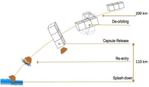
the apparent wind. Once it reaches below 200 km and until the 110 km, specific reaction wheels will change the area of the satellite exposed to the ram direction, allowing to change the ballistic coefficient with a factor of 3, in a few seconds.

Figure 2.1: Re-entry phases

The return of any satellite involves a great deal of uncertainty in what concerns its integrity and impact zone accuracy. The challenge of GAMASAT is to design a simple system for satellite re-entry, defining the impact zone. It is important to choose an impact zone that guarantees safety and yet makes recovery still possible.

To understand the impact zone selection, the following expression gives the kinetic energy of a free falling object on the surface of the Earth:

E= m

2_g

ρCxA (2.1)

Where m represents object mass, ρ represents air density at MSL (roughly 1,2 kg/m3), g represents gravity acceleration (9,8 m/s2), A the area of the capsule exposed to the apparent wind (about 64 cm2) and Cx is the drag coefficient at terminal velocity and at MSL (estimated to be around 0,8).

The re-entry spot needs to guarantee the safety and accessibility to allow for its recovery. For an object’s landing to be considered safe on the ground, its energy is limited to 15 J. A capsule with 0,1 kg has an estimated kinetic energy of around 15 J, which is too close to the limit. Since in this project the capsule will have about 0,2 kg, the algorithm will assume a re-entry with splashdown on water. Therefore it is planned to land within the Exclusive Economic Zone (EEZ) of Portugal exclusive of the Atlantic.

6 Project Overview

2.4.2 Actuation

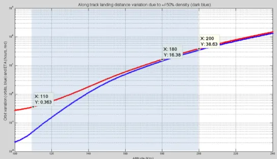
Active control of the satellite will occur between 200 km and 110 km. The following chart can help understand the altitude range were it make sence to preform re-entry control.

The blue line represents a simulation of the along track variation of the landing point given a +/- 50% drag force variation relative to standard conditions (either due to attitude or air density variation), in units of orbits.

The red line represents the remaning flight duration, in units of hours.

Figure 2.2: Distance variation with +/- 50% density variability

Above 200 km the uncertainty is still too high for it to be worth spending control energy, whereas below 110 km the capsule landing region variability is already limited to 500 km along track, and the satellite is just a few minutes from re entry. Cross-track variability is an order of magnitude lower than a long-track variability.

Actuation will occur in cycles of 30 minutes, each cycle initiating with a new GPS reading. For energy consumption management, the onboard GPS receiver will be operated temporally, having been determined that 30 minutes intervals between observations is adequate to maintain a suitable ephemeris (the satellite will periodically computes and broadcast its own ephemeris in the format of Two-Line Element (TLE) [21].

One of the larger faces will be exposed to the apparent wind during a Tontime interval and then

the satellite will be returned back to the normal attitude (smaller face aligned with the apparent wind). This rotation will occur below 200 km until the 110 km, specific reaction wheels will change the satellite exposed area in a few seconds and adjust the ballistic coefficient with a factor of 3.

Adjusting the duty cycle (Ton against the duration of the cycle) allows to actively control the

2.4 Challenge Approach 7

wheels will be employed. These will have significant actuation effectiveness, but low accuracy, since upon rotation the Attitude Determination and Control System (ADCS) will perform any required fine-tuning.

2.4.3 Control Algorithm

The magnitude of Ton will be computed at the beginning each cycle, by the algorithm that

uses the information collected from the updated TLE and predicts the landing spot. A simulation routine computes a landing location for given Tonand given density variations of the atmosphere.

This algorithm assumes that the Ton intervals have an average value of 25% for the following

cycles and that the capsule is released at 110 km. This algorithm results from simplifications of more elaborate procedures, yet giving a sufficiently accurate forecast. It also includes some corrective parameters that will increase accuracy based on previous data.

The optimal Tonis chosen as a way of minimizing cost function that includes a blend of average

landing (stochastic solution) and also a worst-case scenario for the possible drag variations.

2.4.4 Re-entry capsule

The entry capsule will be release from inside the satellite, with a shape designed for re-entry. Built using a heat-resisting materials, this capsule will have a minimal payload, consisting of a radio transmitter, battery and basic sensors (temperature, acceleration and rate of turn). It will also have an off-the-shelf miniature GPS receiver to be used after the deceleration phase of re-entry and upon falling into the ocean.

The capsule will have the general shape similar to the successful Apollo 11 used in one of the lunar missions by NASA, with a 9.5 cm diameter and height about 5.5 cm. It will weigh about 0.15 kg, most of it due to the ceramic material that will protect the interior with little ablation. A cork composite ablative material will cover it. Inside the capsule there will be:

• An oscillation dumping mechanism; • Batteries;

• Antennas (2,45 GHz and 402 MHz); • ARGOS Antenna;

• Flash memory with extensive GAMASAT flight data; • Microcontroller;

• GPS; • Solar Panel; • Flash Light;

8 Project Overview

• Infrared;

Chapter 3

State of the Art

This chapter present a brief review on previous works and studies about de-orbiting and re-entry.

3.1

Overview

In the past a number of experiments for de-orbit and re-entry of small and medium sized objects have been performed by the major space agencies.

These experiments can be classified into the following approaches: Miniaturized Apollo style capsules

• Hayabusa • YES 2

Deployable Re-entry Capsules: • IRDT

• NASA inflatable

While the miniaturized Apollo style capsules aim at equipping smaller systems with de-orbit capability, the deployable re-entry capsules aim to allow a medium sized system to bring down even more payload by reducing the mass and volume fraction of the de-orbit device.

Another method to differentiate between the re-entry systems is the method of de-orbit control. While the larger and often more sophisticated capsules like IRDT focus on a classical propellant based re-entry control system this option is often not feasible for the smaller capsules. The fol-lowing different methods have been used:

10 State of the Art

Propellant based re-entry control

• Inflatable Re-entry Demonstrator Technology (IRDT) • NASA inflatable

• Hayabusa

Teather supported re-entry control • YES2

The method of differential drag de-orbit control has been proposed but not yet been imple-mented [3]. Therefore while being comparatively conservative on the actual capsule design the GAMASAT project will excel beyond the state of the art mainly on the field of re-entry control.

3.2

Description of Existing Systems

In the following section the performed experiments of the existing capsules as well as those under development will be explained in more detail.

3.2.1 Inflatable Re-entry Demonstrator Technology - IRDT

Originally the IDT was developed for Russian Mars96 mission. Unfortunately it was lost due to upper stage failure of the mission. The DaimlerChrysler Aerospace (DASA) (an Euro-pean Aeronautic Defence and Space Company (EADS) predecessor company) and Russian Space Company Lavochkin made an agreement in 1998 to commercialize the technology for earth ap-plications. Two experiments were conducted. Unfortunately the two demonstrator flights in 2000 and 2001 were again not successful. The basic idea behind the IRDT was to test the concept of an Inflatable Re-entry Demonstrator. Its aim was to validate the function to enable the re-entry in a small, lightweight and cost-effective way. It was done using an inflatable extension system. This system offers an increase of ratio between volume and mass and is thus able to perform decelera-tion to take place in higher (less dense) areas of the atmosphere which will in result decrease both the mechanical as well as the thermal loads acting on the capsule.

Purpose: The purpose of the project was to design and built a re-entry capsule, that could remain in orbit for a longer time during the re-entry process would reduce dramatically the speed until it lands.

Who: The Inflatable Re-entry and Descent Technology (IRDT) is project developed by the European Space Agency (ESA), Russian aerospace company Lavochkin and DASA, launched into a sub-orbital ballistic re-entry trajectory by the space launch rocket, Volna, fired from a Russian naval submarine positioned in the Barents Sea in the area of Severomorsk, Russia.

3.2 Description of Existing Systems 11

What: The IRDT is a re-entry capsule that increases it diameter during the re-entry. The increase in size was made using an inflatable extension of the cone in two stages. This procedure allows a slower re-entry, reducing the speed from more the 6800 m/sec when separate from the launch vehicle, to 17,12 m/sec of speed when it lands.

When: After two attempt the IRDT was launched for the third time on 7 October 2005 at 10:30.

Status: Despise the failed on the inflammation of the second shield, the demonstrator survived and was recovered.

Figure 3.1: a) IRDT; b) IRDT deployed

• Gross mass: 350 kg (770 lb). • Payload: 250 kg (550 lb). • Height: 1.83 m (5.99 ft). • Diameter: 0.52 m (1.70 ft). • Span: 2.50 m (8.20 ft).

3.2.1.1 IRDT - Involved key technologies

Type of Re-entry Control: After reaching its final altitude the rocket starts to fall rapidly due its weight. The friction with the atmospheric gases during deceleration in the atmosphere causes the shield to heat up and consequently burn. The heating will be more severe the later it will happen during the flight. The reason is that in the lower parts of the atmosphere the density is higher thus the heating is higher. Ideal would be a solution that slows down the capsule while it

12 State of the Art

is still in the higher parts of the atmosphere. This however can only be reached with very large surface to mass ratios. This requires a very large heat shield relative to the payload. To increase the area of the re-entry capsule an inflatable system is used. During re-entry control is made in two stages. The first one is before the capsule be released, were the spacecraft reoriented on its trajectory. After reaching the maximum altitude the capsule will proceed the descent process in which the first inflammation of the shield occurs. This first shield maintains the traveling velocity (˜6.9 m/sec). The second and last control stage occurs when the capsule is at 14 km altitude. At this point the velocity has already been reduced to 230 km/h. Afterwards this system will guaranty a safe landing.

Type of Capsule: Inflatable

3.2.2 Inflatable Re-entry Vehicle Experiment - IRVE

More than 40 years after the idea of an inflatable re-entry capsule was first published the first successful flight has taken place. Developed by NASA, IRVE became the worlds first successful inflatable re-entry capsule [4]. The aim of the project was to build a new kind of lightweight inflat-able spacecraft structure to slow and protect a re-entry capsule during re-entry in the atmosphere at hypersonic speeds.

Purpose: The project was to proof the feasibility to built an inflatable heat shield to slow down and protect itself as it enters the atmosphere at hypersonic speeds. The inflatable acts as an aerodynamic decelerator with a Thermal Protection System (TPS) that guarantee the re-entry survival of the capsule.

Who: NASA

What: IRVE has a mushroom shaped heat shield that is vacuum-packed into a 56 centimeters diameter nose cone. It is launched on a small sounding rocket on Wallops Island, Va.

When: The first launch of IRVE could not be identified in literature. The launch of IRVE-2 took place at 17 August IRVE-2009 together with Black Brant-IX 1399lb Payload in Wallops Island (Canada). After considerable upgrades in performance (apogee altitude, the re-entry capsule mass, improvement on the inflatable shield) the IRVE was launched on 23 July 2012.

With considerable upgrades, sInce the apogee altitude, the re-entry capsule mass, improvement on the inflatable on 23 July 2012 the new IRVE-3 was launched.

Status: Currently the next generation of IRVE is under development. Is expected to be launched in spring of 2014 [5].

3.2.2.1 IRVE - Involved key technologies

Type of Re-entry Control: Based on the same concept that the IRDT. After the rocket achieves the celling height it opens inflatable heat shield. The IRVE has a mushroom shape to increase the exposed area and reduce the re-entry process.

3.2 Description of Existing Systems 13

Figure 3.2: a) IRVE deployment; b) IRDT deployed [6]

3.2.3 Hayabusa

Developed by the Japan Aerospace Exploration Agency (JAXA), the Hayabusa project was designed to land, collect and return with a sample from a small near-Earth asteroid named 25143 Itokawa to Earth for further analysis [7].

Figure 3.3: a) Hayabusa release[8]; b) Hayabusa Replica [9]

Purpose: The purpose of the Hayabusa probe was to conduct an interplanetary flight and return a sample to the earth. After reaching the designated asteroid with a sample was taken and the returned to earth. Inside the probe was a landing capsule that landed and brought back the collected samples from the asteroid.

Who: The project has developed and executed by the Japan Aerospace Exploration Agency (JAXA).

What: The project contain four main steps: first to independently reach the designated aster-oid, second to use a simplified landing device to retrieve a sample, third to autonomously return the probe to earth and fourth to safely land the capsule on ground to allow inspection of the sam-ples. In the context of this mission the re-entry capsule is the most important part. The Hayabusa,

14 State of the Art

re-entry capsule was made of a heat-shielded with a parachute inside. The parachute was released after the critical descent to slow the capsule down after landing in Australia.

When: Launched 9 May 2003, reentered to the Earth atmosphere on 13 June 2010 in a 20 km by 200 km area, in the Woomera Prohibited Area, South Australia.

Status: Despite being damaged during landing the samples inside the capsule remained intact. The mission was deemed a success.

3.2.3.1 Hayabusa - Involved key technologies

Type of Re-entry Control: The Hayabusa capsule had no active control system; all methods to stabilize were passive. This included a low center of mass and careful selection of the cap-sule angle of attack during re-entry obtain form the shape of capcap-sule cover by high performance resistant.

Type of Capsule: Rigid.

3.2.4 Young Engineers’ Satellite 2 - YES2

One of the most ambitious project, where Delta-Utec SRC and with the ESA Education super-vision, challenged students and young engineers all over Europe to design and built a satellite([10] and [11]).

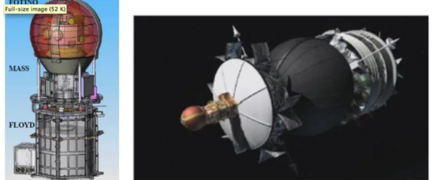
Figure 3.4: a) YES2 contains FLOYD , MASS and Fotino, the spherical re-entry capsule; b) YES2 assembled on FOTON-M spacecraft. [12]

Purpose: The purpose of the mission was to build a low-cost capsule that would return from space to Earth, without the use of any means of propulsion. Instead it was hold and control by a 30 km long and 0.5 mm thin tether, which would lead to a safety land in a pre-determined location.

Who: Build for 450 European students; the project was part of a ESA’s and Foton-M3 mission. What: YES2 is constituted in three components: the Fotino capsule, a Mechanical data Ac-quisition Support System (MASS) and a Foton Located YES2 Deployer (FLOYD). The Fotino is encased with an ablative material, to protect the scientific equipment and the parachute system inside, as it returns to Earth. At the right moment the Fotino capsule is release from the four straps

3.3 De-orbiting 15

that hold it to the MASS. FLOYD is connected with the MASS by a 30 km of 0.5 mm thick tether. Inside of the FLOYD is a robotic spacecraft Foton-M3, which will eject MASS and Fotino towards Earth.

When: Launch on 14 September 2007 in Kazakhstan the YES2 was deployed and release the re-entry capsule on 25 September 2007 to reach Kazakhstan area[13].

Status: Successful

3.2.4.1 YES2 - Involved key technologies

Type of Re-Entry Control: The re-entry will be control for a 30 km long tether. Type of Capsule: Rigid

3.3

De-orbiting

Reduce space debris, recover information or simply due the technological evaluation are some reasons for the studies on the development of the satellite de-orbiting. Depending on the reason and atmosphere layer that the satellite will be in orbit the approach is different.

Some approaches have been made by a control system with propulsion, but requires a more complex systems to deal with the instability induce by the liquid sloshing of Residual fuel. Other example was presented, in the 2nd IAA Conference on University Satellite Missions and Cube-Sat Workshop, suggesting a control made by a four wing moving independently and thanking advantage of the drag coefficient.

3.4

Re-entry

In order to allowing a larger area for the impact zone, the object needs to respect the limit of 15 J, and the easy way to do it is increasing the ratio between the dimension and weight. That was one of the approaches of the ESA project, IRDT. Where the capsule with a 140 kg makes its first increase of the diameters of 80 cm to 2,3 m and then to 3,8 m.

On May 9th, 2005, the unmanned Hayabusa was launched, to collect and return a sample of a small asteroid. A few months afterwards, near the asteroid, the sample recovery was scheduled. Once the satellite was on the return trajectory the re-entry capsule was released. On June 14th, 2010 the capsule was successfully recovered with the help of a GPS receiver and a rescue team that surrounded an area of 20 Km by 200 km in the South Australia.

NASA launched the Inflatable Re-entry Vehicle Experiment (IRVE-3) to test a space capsule with an inflatable outer shell system. An inflation system pumped nitrogen into the IRVE-3 ex-panded the inflatable system, increasing the capsule size to about 10 feet diameter. The shell slows and protect hypersonic speed during planetary entry and descent, or as it returns to Earth.

The landing spot was the coast of North Caroline, on Atlantic Ocean.

A similar approach that will be presented in this thesis was developed in the Young Engineers’ Satellite 2 (YES2) project. On September 14, 2007, was launched 40 ESA experiment with a

16 State of the Art

mission to experiment a 12 days in orbit of zero gravity. One of the experiments was the YES2, a 36 kg student-built project that was deployed September 25, 2007 with objective to release a small spherical re-entry capsule and reach the Kazakhstan. The final mission experiment did succeed and even establish a world record for the longest artificial structure in space, but any signal was received form the capsule after the re-entry and it was never been recovered, meanly calculation indicates the Aral Sea has the landing area.

Chapter 4

De-orbiting Control

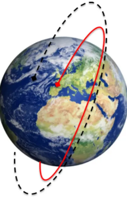
The satellite trajectory is described by its orbital parameters. In an ideal situation without disturbances the orbit would prevail infinitely. However in reality the satellite is affected by a number of disturbances of which in low earth orbit the atmospheric friction is the most severe. This friction can be reinforced by changing the attitude generating trajectory relative to the initial trajectory has a faster altitude decrease rate. There are a number of conditions that influence the trajectory. The two main factors are: vertical density profile of the atmosphere and resulting drag force. In the following figure the effect is presented:

Figure 4.1: Drag force effect on the trajectory. Lower drag force overshoot the landing (black). Higher drag force, faster de-orbiting (red)

For any satellite on a space mission is very important to study the drag and atmospheric condi-tion. This is done to reduce the influence in the trajectory. Since the GAMASAT does not carry a propulsion system the possibilities of influencing its trajectory using the state of the art are limited.

18 De-orbiting Control

In order to allow the new method of differential drag to be working it is required to autonomously calculate the satellites decent during de-orbiting. Its one of the aims of this study to to understand the influences on the satellite trajectory and to use this knowledge to influence the location and trajectory of the satellite up to the moment of the releasing the capsule. The findings of this study will be presented in the following sections of this document.

4.1

Atmosphere - Vertical Structure

The atmosphere vertical structure is described by the following parameters: air density, tem-perature, pressure and molecular mass. The distribution of each parameter can been seen in the following figure:

Figure 4.2: Atmosphere Vertical structure

The density of Earth’s atmosphere is a combination of the pressure and molecular mass. The atmosphere is constituted of gases that surround our planet.

These gases consists of a combination of numerous atoms and molecules. The number of at-mospheric particles or the molecular mass decreases with altitude, decreasing the pressure leading to a decreasing of the air density. This can be described using to relation between pressure and density. In approximation the atmosphere density can be described by the model of the ideal gas. It relates between relate density ρ, pressure P and temperature T:

ρ = RT

PMmol

(4.1)

4.1 Atmosphere - Vertical Structure 19

The four parameters are connected by the formula above 4.1. By solving the equation the density can be described it as a function of pressure and temperature. The temperature has to be analyzed in more detail as it not only depends on the gases but on other external factors. These factors will be described later in this document.

4.1.1 Density

The atmosphere is in equilibrium of gases that are constantly flowing upward by the internal pressure and being forced downward by the gravity. This keeps the atmosphere in a hydrostatic balance. The pressure is higher with lower altitude. This effect can be experienced by everyone who has already climbed a mountain. The reason for this effect is that with every meter gained above ground the mass above oneself is smaller thus is the pressure.

Analyzing the pressure variation in an infinitesimally way, as shown in the figure below, comes the following equations:

Figure 4.3: Pressure vs gravity

P= − m.g

dA (4.2)

for the mass we have:

m= ρ.V (4.3)

and the volume comes as:

V= dA.dz (4.4)

leading us to:

20 De-orbiting Control

The expression above indicates the pressure, not taking in to consideration gravity or/and density variation which is true in the Earth surface, but it becomes incomplete for the atmospheric pressure evaluation. Therefore for a valid atmospheric pressure expression and it variation, we need to consider a density and gravity variation with altitude:

dP

dz = − ρ(z) g(z) (4.6)

The atmospheric pressure is approximately given by:

P= p0.e

−g(z).Mmo(z) h_{R T(z)}

(4.7) Being the pressure scale height, H defined by:

H(z) = R T(z) g(z) Mmol(z)

(4.8)

Relating the equation4.7and4.8comes:

P= p0.e − h

H(z) _(4.9)

The variation of density with height can be derived similarly, resulting in:

ρ = ρ0.e − h

H(z) _(4.10)

This equation it is only valid where the temperature remain constant with height in a vertical structure. This is the case of the thermosphere which is the layer of interest for this study. This invariability lead us to a density scale height equals to the pressure scale height. If this would not be the case we would otherwise need to consider that variation of the temperature in the calculation of the density scale height.

Comparing equations4.9and4.10we see that there is a similarity, which was expected from the analysis of Figure4.2. However since temperature shows a variation that is almost equal to the gain of the density over the pressure the effects of temperature needs further analysis.

4.1.2 Temperature

A more detailed way to describe the temperature variation can be achieved by atmospheric models. In this document, as shown in Figure4.4, a NRLMSISE- 00 model was used. This model

4.1 Atmosphere - Vertical Structure 21

takes the temperature variation 400 km over Delft, in the Netherlands in to account . It shows the density variations over a solar flux cycle, between 2000 and 2006.

This section will present a brief review about the impact of temperature in the atmosphere dynamics and consequently in the air density.

For the purpose of this thesis only the variation until 200 km will be analyzed.

Figure 4.4: Density variation and temperature with altitude, according to the NRLMSISE-00 model [14]

Temperature is a measure the thermal energy of a particle due to micro vibrations. These vibrations increases the chances of collision between particles and objects consequently increases the temperature of these objects.

In the atmosphere the Sun is responsible for the increase of the ambient temperature. Although the atmosphere temperature reaches more than 1000◦Cin the thermosphere collisions are scarce due to the lower density, making the thermosphere bearable.

By the ideal gas law the temperature T is given:

T = P V

n R (4.11)

with P being the pressure, V the volume, n the number of moles and R the universal gas constant.

22 De-orbiting Control

4.1.2.1 Overview

The Sun energy is the source for the ambient temperature. The energy flux of the sun can be approximated as a black body source with 5800 K [23]. According to the Planck law it transmits energy from low energy radio waves to high energy X-ray.

Figure 4.5: Black body Curves [18]

As it can be seen the peak of the sun activity is at 500 nm [23]. The level of radiation that reaches the earth and its atmosphere is dependent on a number of factors. These factors will be described in the following sections. It reaches the atmosphere through ultraviolet radiation and X-radiation, heating and ionizing the atmospheric gases.

The levels of radiation change with latitude and longitude and decrease the distance from the Sun and change with the amount of solar activity.

4.1 Atmosphere - Vertical Structure 23

Temporal Variation:

Temporal variations include diurnal variations, seasonal cycles and long periods. These vari-ations directly influence the change of electron density. Diurnal varivari-ations are caused by changes of solar radiation, which disappear at night.

The seasons also influence the variation of the electron density due to the change of the zenith angle of the sun and the intensity of the flow of ionization. In equinox, the effects of the iono-sphere are larger, whereas in solstice, the effects are minor.

Location:

The geographical location also influences the variation of electron density, because the overall structure of the thermosphere it is not homogeneous. It changes with latitude, due to the variation of the zenith angle of the Sun, which influences directly the level of radiation, which changes, in turn, the electron density in the ionosphere. The influence of longitude, due to the non-coincidence of the magnetic and geographic poles, is sensitive only in the higher regions.

Solar activity:

The sun magnetic activity varies cyclically in periods of approximately 11 years.

These activities are associated with occurrences of sunspots, and the increase of ionization is proportional to the number of spots. The period of maximum solar activity caused an increase in the number of sunspots and consequently, the number of electrons present.

At the core of the Sun with high temperatures, density and pressure does the process of nuclear fusion of hydrogen into helium. The energy that is generated in the core is transported by radiation to a radiative layer that surrounds the core. Between the radiative layer and the next layer it as an interface were the sun’s magnetic field is generated. The next layer is the convection zone were power transmission is by convection, transporting the less dense material to the Sun’s surface. The last layer, corona layer consist of plasma. The high temperature ionized gases that escape through coronal holes, creating the Solar Wind that is responsible for the geomagnetic storms. The geomagnetic field controls of the ionized gases movement, so the geomagnetic storms will dramatically change it motion and consequently will affect the density. Higher the geomagnetic storms, higher will be the air density.

Equation 4.11show that by increasing the temperature and for a same volume, the pressure will consequently increase. Taking that conclusion to the equation4.1 it is obvious that the air density will decrease.

In case of increasing the temperature in same pressure the gases will rise. Followed by the equation4.3the density will consequently increase.

24 De-orbiting Control

Greenhouse effect:

The temperature n stable state of any object in an orbit around sun depend on a number of factors. The main factors have been described earlier. There is however another factor that is resulting from the atmosphere itself. For an spherical body in earth orbit the temperature would only be dependent on its color, hence the amount of absorbed to emitted heat. This is shown by the Wien’s displacement law[15]:

λmax(nm) =

2.897(8)106(nm)

T(K) (4.12)

The amount of radiation absorbed depends on the reflectivity of the planet, designated of Albedo (Al) and the Solar constant of the planet governed by the equation:

Powerabsorbed= AreaSolar(1 − Al)

(distance)2 (4.13)

In case of emitted radiation the equation that describe it is the Stefan Boltzmann law: Power

Area = σ T

4 _(4.14)

Another difference between the Power emitted and absorbed is the Area. Assuming a uniform temperature all around the world, the emitted power is made all around the surface of the planet, so the Area will be 4πR2. In case of absorbed radiation, only the area that is faced to the Sun is absorbing, there so the Area is πR2.

Equating these two equation4.13and4.14the equilibrium temperature can be calculated as a result of incoming and outgoing fluxes.

(πR2)Solar(1 − Al) = (4πR2)σ T4 T = 4 r Solar(1 − Al) 4σ (4.15) SolarEarth= 1370W /m2[16] AEarth≈ 0.31[17]

Based on these factors it can be calculated that the average temperature of earth without any further effect would be ≈255 K (−18◦C). Since the actual measured average temperature of earth is actually in the range of ≈288K (+15◦C) this indicates another influence factor. This factor is the green house effect of atmosphere. While the man made green house effect has been matter of discussion in the recent years it is an often overlooked fact that without the natural green house

4.1 Atmosphere - Vertical Structure 25

effect earth would not be habitable. Since the extension of the atmosphere is directly influenced by earth surface temperature a further look is taken onto it.

Figure 4.6: Earth transparency of atmosphere [24]

Due to the fact that the atmosphere is largely transparent for high energetic visible light but not transparent to thermal parts4.6 of the spectrum that means that on the one hand the energy of the sun can enter the atmosphere on the other the peak of the earth own black body radiation (at 250 K) is in thermal infrared an cannot pass. The source of this natural green house effect is largely the water vapor in the atmosphere. In the recent years additional man made effects, largely CO2, by burning of carbon based energy sources has been introduced to the atmosphere. This further reduces the transparency of the atmosphere. With regard to the focus of this study this has two effects. First the temperature of the lower atmosphere rises due to the inability of thermal radiation (heat) leaving the atmosphere. Secondly due to the reduced transmission the outer layers of atmosphere actually cool down in absence of this heat flux. Thus in contrary to popular believe the atmosphere shrinks and friction decreases. This factor is influencing the time frame of how long a satellite can maintain orbit and its de-orbit. However for the purpose of the study this effect can be considered static.

4.1.2.2 Simplified Model

After describing the properties of the atmosphere it becomes apparent that these values cannot be measured during the re-entry process. For simulation purpose a simplify exponential density model of the atmosphere is enough to describe the satellite dynamics. Therefore the following table is used on the density estimation:

Following the table form Figure4.7the density is calculated for each layer using the equation

4.10. Where the base altitude, h0, nominal density, ρ0, and scale height, H, can be taken from

26 De-orbiting Control

Figure 4.7: Exponential Atmospheric Model [19]

4.2

Drag Force vs attitude

The drag force is the force that opposites the movement of a body on a fluid and it is given by the following expression:

FD=

1 2ρCxAv

2 _(4.16)

The equation quantifies the force imposed to an object with an area A and velocity v and a coefficient of aerodynamics Cx, that crosses a fluid with density ρ.

By the drag force equation it is clear that during the body trajectory only the exposed area and velocity can be controlled, and by decreasing the exposed area or the velocity the drag force decreases.

This relation can be seen in sports as racing sport, ski, horse racing, cars or in the fighter aircrafts by retracting the exposed area of the object/runner to the wind so it can decreases the drag force by reducing the exposed area and increases the speed.

We can also see that the amount of drag force suffered by an object depends on drag coefficient Cx that describes the object aerodynamics.

4.2 Drag Force vs attitude 27

4.2.1 Drag Coefficient

The drag coefficient Cx describe a relationship between the drag force, density, exposed area and velocity that depends only on the object shape. However, since the fluid behavior depends on density and even on velocity different coefficients apply for different conditions. For example, at, higher density (such as at MSL density) the flow of around a object impose modifications to the interaction between air particles, cause such flow to be smooth around the object and causing turbulence at the wake region. As showed in figure4.11.

Figure 4.8: Flow through a Sphere vs Cube

In very low density situations, such as in the thermosphere, particles are so scarce that in-teraction between particles are negligible; therefore the derivation of the drag coefficient in such conditions can be performed by addressing the single interaction of the particles with the exposed are of the object.

4.2.2 GAMASAT Drag Coefficient

As seen previously the higher the altitude the lower the number of particles will be. The number of particle is so low that it trajectory is not affect by each other and so the drag coefficient will be higher.

Unfortunately the exact flow condition that the satellite will be facing within the outer parts of the atmosphere is unknown. To find the approximate value an analysis of the linear momentum and the kinetic energy of possible collision types was made. The type of collision is described by the particles attitude. In a first step the particle attitude is described by the conservation of momentum. Initially a particle, m, with velocity v impact in a satellite, M, at rest, V = 0, as showed in the Figure4.9. After the collision the particle have a new velocity, v0, and the satellite remains at rest.

28 De-orbiting Control

Figure 4.9: Kinetic Energy transfer due the collision

With the conservation momentum and the figure we can take the following equation : m∆v = M∆V m(v + v0) = M∆V (4.17) m= ρAv∆t ρ Av∆t(v + v0) = M∆V ρ Av(v + v0) = M∆V ∆t (4.18) ρ Av(v + v0) = Ma FD= ρAv(v + v0)

Considering that k is the relationship between the particle velocity before v and after v0 the colli-sion.

v0= kv (4.19)

FD= ρAv2(1 + k) (4.20)

Relating the Equations4.16and4.20we have:

ρ Av2(1 + k) =1 2ρCxAv

2 _(4.21)

1

4.2 Drag Force vs attitude 29

Cx= 2(1 + k) (4.22)

It is expected low, α angles between the particle and the satellite. The types of collision can be analyzed according to the particle state after the collision. They can be:

• Perfectly inelastic collision;

• Perfectly elastic and specular collision; • Non-elastic collision.

4.2.2.1 Perfectly Inelastic Collision

The inelastic collision describes the absence of velocity after the collision, so the kinetic en-ergy is not conserved. In this case the particles get stuck in the object surface. This leads to an accumulation of particle in the object surface (e.g. the case of bugs that get stuck in a car window). So physically what happens is:

• velocity before the collision v = v; • velocity after the collision v’ = 0;

Taking to the equation4.19we have a k = 0;

Replacing in the equation4.25leads to a minimum of Cx = 2. 4.2.2.2 Perfectly elastic and specular collision

In a case of complete elastic and specular collision the particles are projected with the same angle that collided with the object surface as the initial trajectory, but in the opposite direction. So the drag coefficient is given by:

velocity after the collision v0= v.cos(2α) substituting in the equation4.25we have:

v0= v.cos(2α) (4.23)

k= cos(2α) (4.24)

Cx= 2[1 + cos(2α)] (4.25)

Taking an α = 0, lead us to a maximum of Cx = 4.

4.2.2.3 Non-elastic collision

In case of a non elastic collision, after the collision the particle is projected with a different energy. In this case the approach is to analyze the conservation of kinetic energy, that is given by

30 De-orbiting Control

the equation bellow:

1 2m(v) 2₌1 2m(v 0 )2+1 2M(∆V ) 2 _(4.26)

Comparing equations4.17and4.26we can see that the kinetic energy corresponds of the mo-ment of inertia multiply by 1₂ the velocity. In case of the satellite the momentum is already low due to the low variation of velocity before and after the collision, so by multiplying by 1₂ ∆V the kinetic energy variation of satellite is negligible compared with that of the particle.

After the collision the particle is deviated from the trajectory with a different velocity, which relates to the initial velocity according to :

1 2mv 2_{= e}1 2mv 02 _(4.27) v=√ev0 ε = √ e (4.28)

The difference between velocity before and after the collision, the k of equation4.19, is af-fected by the coefficient of elasticity or restitution ε . The ε parameterizes the energy that dissi-pates during the collision. The coefficient of elasticity is limited between 0 < ε < 1, limited by a perfectly inelastic collision and elastic collisions, respectively. For typical a non-elastic collision we will have an ε = 0, 3 [20].

Therefore an analysis for a specular and non-specular collision is needed.

Non-elastic collision and Specular collision

In specular collisions the k is given by the equation4.24multiplied by the coefficient of elas-ticity ε = 0.3. There come that:

k= εcos(2α) Cx= 2[1 + εcos(2α)] (4.29) (4.30) For an α = 0 we have: Cxmax= 2[1 + 0, 3(1)] (4.31) Cxmax= 2, 6 (4.32) (4.33)

4.2 Drag Force vs attitude 31

Non-elastic collision and Non-Specular collision

In case of a non-specular collision the particle can take any angle β , as showend in figure4.10, with the surface after the collision limited by the object surface. Leading a given k0of:

k0= cos(α + β ) (4.34)

When collising with the GAMASAT surface the particles are deflected along any angle β ∈ [−π

2; π

2] according to a probability density function given by the possible model:

P(β ) = 1

2cos(β ) (4.35)

Figure 4.10: Non-specular collision

So the new k is given:

k= π /2 Z −π/2 1 2cos(α + β )cos(β )dβ (4.36)

(Details can be f ound in AppendixA.6) k= π /2 Z −π/2 1 2[ 1 2cos(α + 2β ) + cos(α)]dβ k= π /2 Z −π/2 1 4[cos(α + 2β ) + cos(α)]dβ (4.37) k= π /2 Z −π/2 1 2[ 1 2cos(α + 2β ) | {z } = 0 (A.8) +1 2cos(α)]dβ

32 De-orbiting Control

Therefore k is given:

k=π

4cos(α) (4.38)

In this case we have:

Cx= 2(1 + ε[π 4cos(α)]) (4.39) Cxmax= 2[1 + 0.3( π 4)] Cxmax≈ 2.47 (4.40)

4.2.3 GAMASAT Drag Force

It is expected that both collisions specular and non- specular occur, so a weighted arithmetic average between4.32and4.40, has been made to estimate the drag coefficient.

Cx= 0, 5(2, 47) + 0, 5(2, 6)

Cx≈ 2, 54 (4.41)

From there the resulting drag force can be calculated. As explained earlier the GAMASAT is a 3U CubeSat. That gives a ratio between the smaller cross section and the larger one, a drag force of 1: 3; accordingly the drag force of these two section as also a ration of 1:3. Therefore the the projected landing area can be redefined by switching between the two cross sections. By controlling the actuation time of the two states, will take us to a better altitude for the capsule release.

The proposed process works as follows. In a first step the orbit position, velocity and time are measured using a GPS receiver. This position value is then used to update the predictions for the landing area. Depending on whether the landing area is undercut or overshoot by the satellite an update is made in the relative duration of cross section exposure time of the satellite. The time between two measurements is 30 minutes thus is the resulting cycle time. Switching between the two cross section is performed by rotating the space craft by 90◦.

4.3

Re-entry forecast

The re-entry forecast is essential to correctly apply the control strategy.

The main purpose of the algorithm is to optimize the time for the exposure of the larger cross section of GAMASAT. The estimation and optimization is based on an simplified model that predicts the landing point.

4.3 Re-entry forecast 33

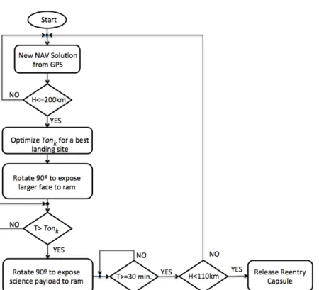
Figure 4.11: Flowchart of De-orbitng Control Algorithm

4.3.1 Time of Control

At the beginning of each cycle GPS readings are taken. Based on the new navigation data the the algorithm calculates the number of orbits until reach the release zone. The release area is the point in the orbit from which the capsule will reach the desired landing area with further steering operations.

With the purpose of reduce the difference between the satellite position and the release area, a time Ton for the larger exposed area is calculated. The differential drag will work with two

states. A small and a big surface area. The difference between those is a factor of three. By exposing the larger surface the satellite is decelerated thus its overall energy is decreased (sum of the potential and kinetic energy). Therefore with this method the satellite will fall faster to the ground. However by decelerating the satellite will go to a lower orbit which in contrast will increase its orbital velocity. Hence relative to the release area the satellite will overshoot. This results in a seemingly paradoxical situation that decelerating the satellite will make it catch up with the release area and accelerating thereby increasing the orbit and decreasing the velocity will make it fall back. Keeping this in mind the algorithm calculates the Tontime. That means the time

in each 30 minutes control interval which exposes the larger surface area.

In order to have the maximum capacity to act on the crash site, the ideal is that the average value of the control is at mid scale. In accordance to this a Tonwith a duty cycle of 50%.

34 De-orbiting Control

However, this would correspond to quite wasting life of the satellite and wasting time with the scientific payload pointed to the apparent wind. Thus, we use the value of 25% as an average between the optimal value in terms of acting ability (50%) and the optimal value in terms of performance of the satellite (0%).

4.3.1.1 Optimize Time of Control

The algorithm computes the Ton time for the current cycle between 0 and 25 minutes. This

calculation is based on the new landing area and based on he assumption that on the next cycle Ton

will used 25% of the 30 minutes cycle.

Previous simulation showed that would take ≈ 5 seconds for the algorithm calculate the Ton.

However a less capable microprocessor is expected to be use, increasing the time for the calculus. Assuming that the microprocessor will be 100 times worst the first 5 minutes will be for the calculation.

Figure 4.12: De-orbiting Control cycles

4.3.2 De-orbiting Control phase

The de-orbit control phase is the time during the re-entry phase in which the satellite actively alters its descent path in order to land in the desired landing zone. This is done using the differential drag method. As explained earlier this control takes place between 200 and 110 km orbit height. In the following the control mechanisms will be explained in detail.

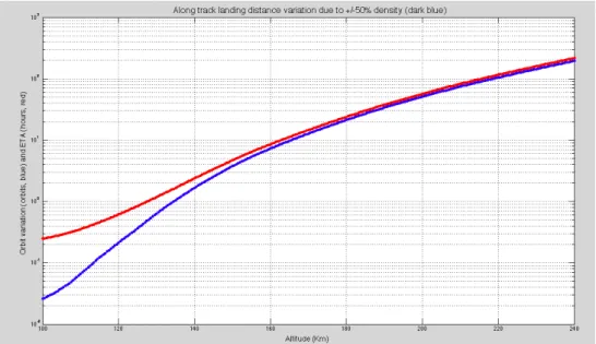
Analyzing the orbit properties shows that the higher the orbit the more control cycles can be done. However analysis also shows that due to higher inherent uncertainties above 200 km there is no point in performing de-orbiting control above such altitude. This means that even if the satellite is correctly actuated the remaining errors will not allow to guarantee the landing in the predicted area. This is shown in Figure4.13. On the other hand for orbits below 110 km there is only very little time left as the satellite will de-orbit within a few minutes. Thus the actuation is too limited and landing region variability will result in an error of 50 km cross-track and 500 km along track. Therefore for a efficient control, the actuation needs to be performed between the 200 and 110 Km.

4.3 Re-entry forecast 35

Figure 4.13: Orbit vs Altitude (red - density without variability) (blue - density with +/- 50% of variability)

Actuation will occur in cycles of 30 minutes, each cycle initiating with a new GPS reading. For energy consumption management, the onboard GPS receiver will be operated sporadically, having been determined that 30 minutes intervals between observations is adequate to maintain a suitable ephemeris [21].

In each cycle, the satellite will rotate 90◦to expose one of its larger faces to the apparent wind, maintain that attitude for a time interval of Ton minutes and return back to the normal attitude

(smaller face aligned with the apparent wind). This rotation will increase the exposed area 3 times, decreasing its ability to overcome air resistance, designated as ballistic coefficient of the satellite. Adjusting the duty cycle Ton against the duration of the cycle allows to actively control

the re-entry location. In order to perform such rotation in a short amount of time (few seconds), specific reaction wheels will be employed. These will have significant actuation effectiveness, but low accuracy, since upon rotation the ADCS will perform any required fine-tuning.

4.3.3 Control Strategy

This is necessary as the conditions influence the state of the capsule and shall therefore be included in the simulations. The algorithm that is used to estimate the time for the larger cross section considers three main guidelines :

• At cycles of 30 minutes new NAV solution are given by the GPS and so, at each cycles new Tonwill be calculate;

36 De-orbiting Control

• The capsule will be released at 110 km of altitude.

4.3.4 Release of Capsule

When the satellite reaches the altitude of 110 km the control is stopped. From there on only the capsule specifications are used until it reaches the Earth surface.

4.4

Simulation

From the chapter 4.1 (Vertical Profile of the atmosphere) the relevant formulas to describe the state of the environment has been described. In chapter4.2(Drag Force vs attitude) formulas describing the resulting drag of the satellite and later the capsule have been identified. Figure4.14

shows the overall scenario and the parameters.

Since these equations are very difficult or impossible to solve by analytical means a numerical solver is used. In the following sections this solver is described in detail. Based on the influence parameters the different interdependencies were identified. The resulting block diagram can be seen below:

Figure 4.14: Block Diagram

4.4.1 Runge-Kutta method - Overview

Runge-Kutta method is a numerical analysis, to solve ordinary differential equations. For a given initial condition 4.42and a function that describe how a variable changes relatively to another variable, Equation4.43the Runge-Kutta solve it giving the new conditions, by recurrence