Monopoly behavior with learning effects and capacity constraints

WORKING PAPER SERIES

CEEAplA WP No. 06/2008

Monopoly Behavior with Learning Effects and

Capacity Constraints

Ricardo Cabral

Monopoly Behavior with Learning Effects and

Capacity Constraints

Ricardo Cabral

Universidade da Madeira (DGE)

e CEEAplA

Working Paper n.º 06/2008

Maio de 2008

CEEAplA Working Paper n.º 06/2008

Maio de 2008

RESUMO/ABSTRACT

Monopoly Behavior with Learning Effects and Capacity Constraints

Using a model motivated by the adoption of new process technology in the

semiconductor industry, this paper analyzes dynamic monopoly behavior with

endogenous learning-by-doing and capacity constraints. The analysis shows

that the monopoly invests in learning early-on by producing at higher rates than

the static optimum. In addition, it invests in more manufacturing capacity than

the static optimum in order to be able to learn faster. Furthermore, in order to

prevent prices from falling too rapidly it leaves some capacity idle as the

technology matures and learning externalities becomes negligible. Finally, the

monopoly may set price below marginal cost when demand is large or growing

rapidly.

JEL classification: L11, L12, L63

Keywords: Semiconductor industry, dynamic monopoly behavior,

learning-by-doing

Ricardo Cabral

Departamento de Gestão e Economia

Universidade da Madeira

Edifício da Penteada

Caminho da Penteada

9000 - 390 Funchal

Monopoly behavior with learning effects and capacity

constraints

Ricardo Cabral* (Universidade da Madeira e CEEAplA)

May 2nd, 2008

Abstract

Using a model motivated by the adoption of new process technology in the semiconductor industry, this paper analyzes dynamic monopoly behavior with endogenous learning-by-doing and capacity constraints. The analysis shows that the monopoly invests in learning early-on by producing at higher rates than the static optimum. In addition, it invests in more manufacturing capacity than the static optimum in order to be able to learn faster. Furthermore, in order to prevent prices from falling too rapidly it leaves some capacity idle as the technology matures and learning externalities becomes negligible. Finally, the monopoly may set price below marginal cost when demand is large or growing rapidly.

JEL classification: L11, L12, L63

Keywords: Semiconductor industry, dynamic monopoly behavior, learning-by-doing

*

Departamento de Gestão e Economia, Universidade da Madeira, 9000-390 Funchal, Portugal, e-mail: rcabral@uma.pt.

The author gratefully acknowledges financial support from PRAXIS XXI, FCT, Portugal. I appreciate comments by Santiago Budria, Henry Chappell, Günther Lang, John McDermott, and participants of the Industry Economics Conference 2005, La Trobe University, Australia. The usual disclaimer applies.

1. Introduction

It is well known that the semiconductor market experiences wide swings in prices and that substantial price declines over time are typical in this industry. For example, in the competitive DRAM market, prices for some types of DRAM chips fell in 2001 by more than 80% to a point where most manufacturers were selling under (marginal) cost.1 More

interestingly, Intel, which had an 80% market share of the PC compatible microprocessor market in 19982 and arguably significant market power, also aggressively lowered the price of

its microprocessors, even for models where it did not face direct competition. More recently, the LCD (liquid-crystal-display) flat screen industry, whose technology is based on semiconductors (transistors) and the manufacturing processes are also characterized by learning-curve economies (Linden et al., 1998), has experienced rapid growth in output and revenues and seen large outlays in manufacturing capacity, accompanied by falling prices and disappointing industry profitability.3

Several explanations have been offered for the observed industry performance. Linden et al. (1998) argue that uncertainty about demand growth and future supply capacity may result in price fluctuations leading to periodic overinvestment in capacity. The literature on learning-by-doing (Spence, 1981; Fundenberg and Tirole, 1983; Dasgupta and Stiglitz, 1988; Cabral and Riordan, 1994; Siebert, 2003) focuses on the dynamic externalities associated to learning and resulting implications to industry performance, in the context of models of imperfect competition with strategic interaction, such as that the industry may be a natural monopoly (Dasgupta and Stiglitz, 1988) or that there may be self-reinforcing market dominance (Cabral and Riordan, 1994), and excessive learning and competition (Fundenberg and Tirole, 1983; Cabral and Riordan, 1994).

This paper’s dynamic monopoly model suggests a complementary hypothesis: if in addition to learning investments in manufacturing capacity are lumpy4, then, relative to the

static optimum, there is over-investment in capacity and in initial production levels with a new semiconductor process technology. In the model developed here, a larger capacity investment

(i.e., larger scale) allows the firm to produce more output and therefore to learn more rapidly.5

As a consequence of the dynamic externalities associated with learning and lumpy capacity, the monopoly reduces price over time and operates with excess capacity as the technology matures, in order to prevent prices from falling too rapidly. Interestingly, a social planner behaves similarly but always produces strictly more and invests in more excess capacity than the monopoly. Such predicted behavior is consistent with anecdotal industry evidence. Further, as in Dasgupta and Stiglitz (1988) and Siebert (2003), the monopoly may set price below (“static”) marginal cost. Finally, the model demonstrates the role of learning as an investment to lower future marginal costs, bringing into light its intertemporal effects (Spence, 1981).

This paper is organized as follows: Section 2 provides the background of the analysis. Section 3 develops the theoretical model. Section 4 and 5 present the numerical and welfare analyses, respectively. Section 6 concludes.

2. Background

The semiconductor industry is characterized by rapid technological change6, significant

learning effects, and large capital outlays in production capacity. Both the learning effects and the capital outlays are typically specific to the manufacturing process technology (Flamm, 1993; Siebert 2003; Cabral and Leiblein, 2001). For example, early in the life cycle of a new manufacturing process technology, as much as 90 percent of output is flawed and must be discarded; once greater production experience has been gained this failure rate can fall to under 10 percent (Irwin and Klenow, 1994; Dick, 1994). As in earlier research, past cumulative output is considered here as the appropriate measure of experience. Thus, as cumulative output rises, learning-by-doing results in increasing production ‘yields’, that is, increasing percentages of usable semiconductor chips. Consistent with anecdotal industry evidence, several empirical analyses have found significant learning effects in the semiconductor industry. For example, the European Semiconductor Industry Association estimates a 30% average cost decline with each doubling of cumulative output in semiconductor chip manufacturing (ESIA, 2006). Irwin and Klenow (1994) estimated a 20% average learning curve for the 4K through 16MB DRAMs.

The OECD (Ypsilanti, 1985) found that 80% of the manufacturing marginal costs for 64K DRAMs arose from yield factors.

Prior literature has offered several relevant insights on the consequences of learning-by-doing. Spence (1981) shows that with learning social optimum requires pricing below “static” marginal cost. Fudenberg and Tirole (1983) argue that learning is a strategic variable and the oligopoly interaction will result in too much learning. Dasgupta and Stiglitz (1988) demonstrate that a monopoly may set price below marginal cost and that if learning is firm specific, the industry is a natural monopoly. Cabral and Riordan (1994) argue that market dominance can be self-reinforcing but that there can be too much learning leading to “excessive” competition. Siebert (2003) shows that learning effects are not constant over the technology life cycle, but rather are more significant when the new technology is introduced, and that this effect may lead to below-cost pricing during the initial stages of the new technology. Cabral and Leiblein (2001) find significant short term intergenerational learning effects between subsequent technologies but no long term effects, indicating that learning accumulated rapidly becomes obsolete.

An additional issue addressed in this paper concerns the effect of capacity constraints on dynamic firm behavior. Earlier research (Gilbert and Harris, 1984) shows that, if firms always produce at full capacity, Cournot competition will eliminate profits, as each firm will build a new plant as soon as it can earn non-negative profits. Flamm (1993) argues that the assumption that firms are not capacity constrained results in models that do not reflect the industry reality well and that constraining firms to produce at full capacity may restrict them to sub-optimal paths. Gabszewicz and Poddar (1997) analyze the impact of uncertain demand in a two-stage duopoly game with capacity choice in the first stage and Cournot competition in the second stage, and show that the firms will invest in excess capacity. Besanko and Doraszelski (2004) look at the persistence of asymmetric firm sizes and show that firm behavior and industry evolution depend on whether the firms compete on quantity or price and in the latter case show that a lower degree of irreversibility in the investment leads to more aggressive

competition. Pacheco-de-Almeida and Zemsky (2003) argue that the existence of a time lag between the investment decision and production, leads to a strategic firm preference towards incremental capacity investments.

3. Model

The model analyzes the adoption of a process technology by a semiconductor producer. The typical firm’s profit function incorporates the role of manufacturing defects as well as output rates and capacity constraints, using an approach proposed by Flamm (1993). Thus, (net) output is a function (product) of the manufacturing yield, capacity utilization rate, and overall capacity, but the costs are determined by gross output, i.e., include also the costs of manufacturing defective devices.

The model analyzes the behavior of a monopoly that faces no threat of competitive entry that seeks to maximize its profit in adopting a new process technology. The monopoly learns from its own manufacturing output in that its manufacturing process yield rises with greater cumulative output. The monopoly has one choice functional, the capacity utilization rate, and two choice variables, the adoption date and the capacity of the new plant. The monopoly is not constrained to produce at full capacity at all times, although the profit maximization condition implies it will do so for at least some time.

In addition, production with the new process technology after Tf, is no longer

profitable, a proxy for the exogenous arrival of “newer” lower-cost process technologies that make the investment in production capacity obsolete after a few years. The model also assumes that the monopoly cannot store output between any two periods, i.e., the output is sold immediately. Given the pace of technological change in the semiconductor industry, this assumption is not unrealistic.7

The monopoly’s problem can be specified as follows:

[

]

0 f 0 T r 0 T T t r e K) , F(T dt e K u c y p max u K, , 0 T ⋅ − ⋅ − _{⋅ − ⋅} ⋅ ⋅ ⋅ − ⋅ = ∏

_∫

(1) s.t.

,

0

,

0

,

0

,

1

0

,

)

(

0 0 0

≥

≥

≤

≤

≡

≡

≤

≤

=

π

K

T

T

y

q

q

u

E

T

E

f s d

where u=u(t) is the capacity utilization rate, which is constrained to [0,1], T0 is time of adoption

of the new process technology, F(T0, K) is an exogenous investment cost function, and K is the

scale of adoption or capacity of the new plant. p=p(t) is the market price, c is the unit production cost for raw chips, and y=y(t) is the monopoly’s output. Further,

K u w y t E&( )= = ⋅ ⋅ , (i)

is the production function

w=

φ

0⋅Eφ

1 _(ii)

is the fabrication yield, and

qd =a t ⋅p−

( ) ε (iii)

is an isoelastic demand function as in Flamm (1993), Spence (1981), and Baldwin and Krugman (1987). In these equations, w is the percentage of “good” chips (i.e., the yield) of the manufacturing process, and a(t) is a demand shift function, reflecting the growth in demand level for semiconductors over time. The model state variable is E(t), which is the cumulative production, i.e. our proxy for learning which we refer to as experience throughout the text, with

E(T0)=E0>0. The remaining parameters are described in Table 1.

The problem is solved using optimal control theory and the maximum principle to find the optimal time path for u*(t). The problem’s Hamiltonian function is:

H t E u( , , , )

λ

= G t E u( , , )+

λ

( )t ⋅g t E u( , , )

where G(t,E,u)=

[

p⋅y−c⋅u⋅K

]

⋅e−r⋅t and g t E u( , , )= = =E& y

φ

₀⋅Eφ1⋅ ⋅u K

ε ε 1 1 ) ( ⋅ − =a t y p therefore:

(

)

H t E u( , , , )

λ

a t( ) ε

φ

Eφ u K e r t c u K e r t

λ

( )t

φ

E u K ε_{ε φ} = 1 ⋅ ⋅ ⋅ −1⋅ − ⋅ − ⋅ ⋅ ⋅ − ⋅ + ⋅ ⋅ ⋅ ⋅ 0 0 1 1 ₍₂₎

where λ(t) is the shadow value (i.e., net present value) of an additional unit of experience, or,

alternatively, the amount by which the firm’s profits over the entire planning horizon would increase if current output were marginally higher.

The maximum principle first-order necessary conditions are:

max ( , , , ), [ , ] ( ) H t E u t T u t f

λ

∀ ∈ 0 (3) s.t. 0≤ ≤u 1 (capacity constraint) & E =

∂

H

∂λ

(equation of motion for E)

&

λ

∂

∂

= − H

E (equation of motion for λ)

λ

(Tf )=0 (transversality condition)

and the Hamiltonian is to be maximized with respect to u alone as the choice functional. The transversality condition imposes the requirement that the shadow value of additional experience at Tf be zero, i.e., λ(Tf)=0, i.e., production after Tf is no longer profitable. The maximization of

the Hamiltonian with respect to u results in:

(

)

ε

ε

ε

φ

φ

λ

∂

∂

ε ε φ ε φ −

















−

⋅

⋅

⋅

⋅

⋅

⋅

⋅

−

⋅

=

∨

=

∨

=

⇔

=

⋅

₋ ⋅ ⋅

1

)

(

)

(

*

1

*

0

*

0

₁ 1 1 0 0 1

K

E

t

a

K

E

e

t

K

c

u

u

u

u

H

u

t r (4)

The maximized Hamiltonian function H0 is obtained by substituting u*=u*(t,E,λ),

(

)

* 1 1 * 0 0 * ) ( ) ( ) ( 1 ) ( 0 ) , , ( 1 1 0 0 1 0 1 0 1 1 1 = < < =            ⋅ ⋅ ⋅ + ⋅ ⋅ − ⋅ ⋅ ⋅       ⋅ − ⋅ ⋅       − ⋅ = ⋅ − ⋅ − − ⋅ − ⋅ − − u u u K E t e K c e K E t a e t E c t a e E t H t r t r t r t r φ ε ε φ ε

_φ

_λ

_φ

λ

φ

ε

ε

ε

λ

ε φ ε

Substituting the other first-order necessary conditions in this expression results in:

1 * 1 * 0 0 * ) ( ) ( 1 ) ( 1 ) ( 0 ) , , ( / 1 0 1 1 0 1 0 0 1 1 1 1 1 = < < =                    ⋅ +       ⋅ ⋅ ⋅ − ⋅ ⋅ ⋅ ⋅ ⋅ − ⋅       ⋅ − ⋅ ⋅       − ⋅ ⋅ ⋅ ⋅ − = ⋅ − ⋅ − − − ⋅ ⋅ − u u u e t K E t a K E e E e t E c c t a e E t t r t r t r t r

λ

φ

ε

ε

φ

φ

λ

φ

ε

ε

φ

φ

λ

λ

ε φ φ φ ε φ ε & and 1 * 1 * 0 0 * ) ( 1 ) ( 0 ) , , ( 1 1 0 0 = < < =            ⋅ ⋅       ⋅ − ⋅ ⋅       − ⋅ = − ⋅ u u u K E e t E c t a E t E rt φ ε φ ε

φ

λ

φ

ε

ε

λ

&

Since output is always non-negative, experience can never decrease, that is, E& ≥0. Analysis of the latter expression for E& then suggests that:

ε

ε

φ

λ

ε φ ε

−













⋅

⋅

−

⋅













≥

⋅ −

1

0

0 1

c

E

t

e

r t

( )

and therefore from the previous expressions it follows that, as long the plant is not idle, i.e.,

u>0, then

λ

&

<

0

, i.e., the shadow price (value) of additional experience is strictly decreasing over time, and that E& >0, i.e., experience is strictly increasing over time.

(

)

* 1 1 * 0 0 * 1 ) ( ) ( 0 * 1 1 1 1 0 0 = < < =             ⋅ ⋅       − ⋅         ⋅ − ⋅ = − ⋅ u u u K E t a e t E c MR rt ε φ ε φ

φ

ε

ε

λ

φ

The above expression shows that the dynamic marginal revenue is constant over time in the interior regime, if the discount rate is zero, as argued by Flamm (1993) and Spence (1981); i.e., there is “forward pricing” behavior in the sense that the “true” marginal cost at each point in time is equal to marginal cost at the end of the time horizon.

While the system of differential equations associated with the boundary solution (u*=1) is relatively easy to solve, the same is not true for the more general interior solutions. In the latter case the problem cannot be solved analytically and the convergence of the system towards equilibrium cannot be inferred from the stationary locus of the costate variable and of the state variable, since

λ

&

<

0

and E& >0 everywhere. Finally, the existence of constraints on the control variable creates corner solutions and transitions between the interior and the boundary regimes of differential equations. Therefore, the model was solved numerically, as described in Section 4.1, and the results analyzed for robustness through sensitivity analysis.

Before proceeding to the numerical analysis, it is useful to derive the expression for optimal “static” output if the firm maximizes static profits only, for example if the firm does not consider the impact of learning-by-doing on its future costs, and to compare it with the optimal (dynamic) output. In this case, the shadow price of additional experience becomes zero, λ(t)=0,

i.e., the dynamic externalities from learning cease to exist, and the yield, ω, is constant. This corresponds to a mature-technology scenario, and the analysis simplifies to the static profit maximization problem:

π

= ⋅ − ⋅ ⋅p y c u K

max

π

ω

ε ε ε u a y c y = 1 ⋅ −1 − ⋅

which, assuming an interior solution, results in:

y a c *= ⋅ ⋅ −  

ω ε

_

ε

ε 1 (5)

where y* is the optimal “static” output level for a given manufacturing yield ω. In fact, the numerical analysis below shows that optimal static output is always lower than optimal dynamic output.

4. Numerical Analysis

The numerical analysis is concerned with the production strategy of a monopoly following the introduction of a new process technology. Due to the existence of learning-by-doing, the monopoly production level, is dependent on past cumulative production and the current capacity utilization rate, u(t). In this analysis, it is assumed that only the more interesting type of binding constraint on the state variable will occur (u*(t)=1), since the other constraint (u*(t)=0) corresponds to a situation with no output (plant is idle).

4.1. Methodology

To solve the problem numerically it is necessary to determine the optimal control path for the capacity utilization rate. Any solution to the optimal control problem has the following characteristics: (i) the optimal control path, i.e. the utilization rate path, u*(t), is piecewise continuous; (ii) the optimal state path, i.e. the experience path, E*(t), is twice continuously differentiable, and is strictly increasing; and (iii) the optimal costate path, λ(t), is continuously

differentiable, and is strictly decreasing.

Since there may be one or more transitions in regime among constrained solutions (u*=1) and interior solutions (0<u*<1), and since this is a problem with an initial condition (E(T0)=E0), a free endpoint (E(Tf) is unrestricted), and a transversality condition (λ(Tf)=0), the

numerical solution is determined iteratively. In each transition in capacity utilization rate regime, the state and the costate variables must be continuous.

The problem cannot be solved by backward induction since the state variable has a free endpoint. Thus, the only approach is to depart from a “best guess” for λ(T0), and then iteratively

converge to the solution that also satisfies the transversality condition. A “best” starting estimate of λ(T0) is obtained by solving the constrained regime (u*=1). The model has enough

flexibility to deal with a number of feasible control paths, specifically (i) an interior control path, 0<u(t)<1, for all t∈[T0,Tf], which is not an equilibrium solution since the monopoly could

always increase profits by choosing a smaller plant size; (ii) an initially constrained control path, u(t)=1, with a later transition to an interior solution; (iii) a transition from an interior control path to a constrained control path, and then back to an interior control path; and (iv) a full constrained control path u(t)=1.

By imposing the continuity constraints and the initial and transversality constraints, it is possible to numerically determine the time of transition from the boundary maximized Hamiltonian to the interior maximized Hamiltonian function and vice-versa, for each of the regimes. Once the control path is determined, it is possible to calculate the profitability of adoption given the capacity K and the time of adoption, T0. This procedure is repeated for

combinations of the other choice variables, capacity, K, and time of adoption, T0, to determine

the most profitable choice. The combination of K and T0 that maximizes profits for the optimal

control path is the optimal dynamic firm strategy.

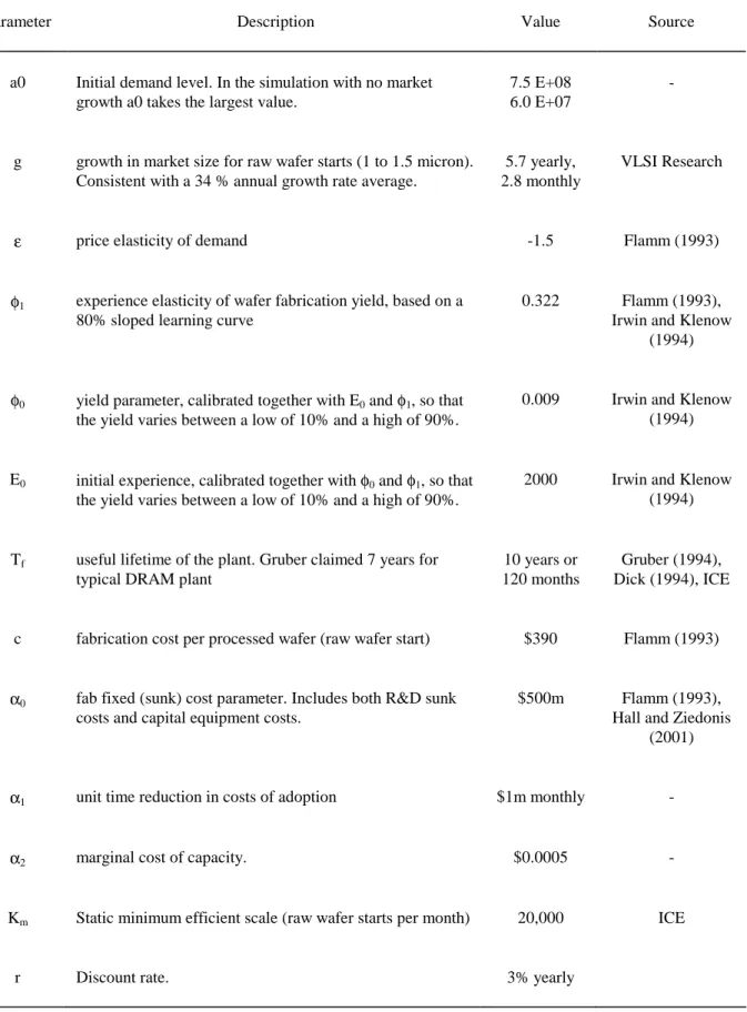
4.2. Numerical analysis with a constant demand level

The first problem is to find the optimal control path that maximizes the firm profitability for a given technology (time of adoption T0=0) and plant capacity. In addition, it is

assumed that the demand level is constant, consistent with mature markets, i.e., g=0 and

a(t)=a0. The graphs of Figure 1 represent the optimal control path, u[t], the optimal state path,

E(t) or e[t], and the optimal costate path, λ(t) (in the graph represented as l[t]), and the

INSERT FIGURE 1 ABOUT HERE

Figure 1(d) suggests that a profit maximizing monopoly will consider the impact of learning-by-doing on future revenue. That is, if the monopoly were myopic, its output path would be ys[t], below the optimal dynamic output path, yd[t]. Learning-by-doing thus increases

the output path relative to the static optimum. The results also suggest that the relative investment in learning as expressed by yd[t]/ys[t] is strictly decreasing, despite the assumption

of a learning curve specification with a constant learning rate, suggesting learning is relatively more valuable during the initial stage of the technology. The intuition is that on the one hand experience gained initially translates into larger absolute cost reductions and on the other hand it reduces the production costs of all units produced afterwards. Furthermore, as Figure 1(f) suggests, at later stages the optimal dynamic output converges towards the static output and the monopoly produces at declining utilization rates, because the present value of future learning-by-doing gains associated with an additional unit of experience continuously decreases. In the limit, when the shadow value of learning is zero, the monopoly’s problem becomes equivalent to the static monopoly problem. Finally, during the entire product cycle, the monopoly sets a price above its static marginal cost and the optimal price path is decreasing (see Figure 1(e)) even without the threat of competitive entry. Note that Siebert (2003) finds empirical evidence for DRAM technology that the learning rate is higher early on. Thus, had the model been specified with a decreasing learning rate as suggested by Siebert (2003), then the monopoly would have an even larger incentive to invest in learning early on.

The monopoly chooses a plant capacity larger than the static optimum, produces at full capacity for some initial period (“ramp-up” production), and later switches to a regime with declining utilization rates as the process yield increases.

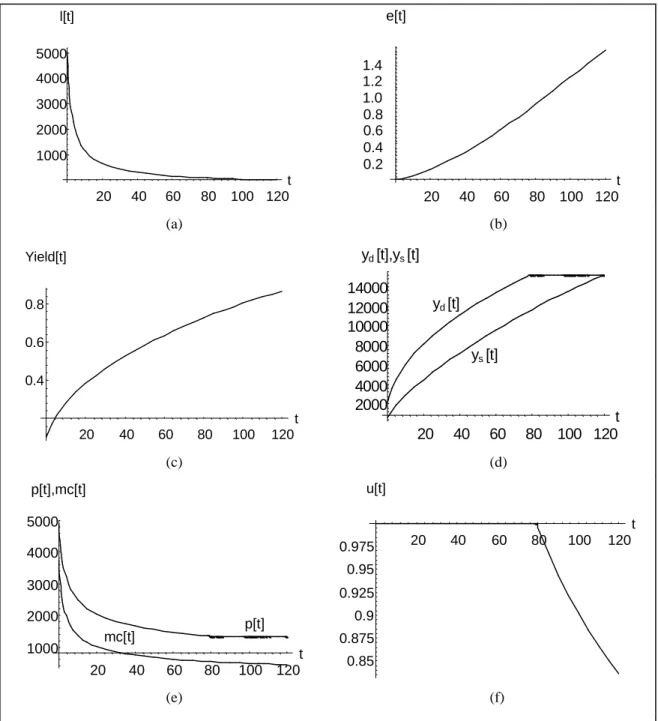
4.3. Numerical analysis with growing demand

In this section, the analysis is enriched by considering the case of an initially rapidly growing market, where the demand curve is shifting outwards with time (a(t)=a0, g>0),

consistent with anecdotal industry evidence (Jovanovic and MacDonald, 1994; ICE, 1990-1995).

INSERT FIGURE 2 ABOUT HERE

Interestingly, if the demand level or growth rate is high, as in the case of Figure 2, the monopoly may choose to set price below marginal cost for some initial period. This result is consistent with the Dasgupta and Stiglitz (1988) finding that a monopoly might set prices below marginal cost in a first period but suggests that Siebert’s (2003) inference that the variance in learning rates over the technology life cycle is driving the result of below-cost pricing is incorrect, since in this analysis learning effects were assumed to be constant.

Furthermore, the analysis suggests that the firm may choose to adopt the new process technology in a plant with a higher capacity than initially needed. In this case there is an initial period where the monopoly does not produce at full capacity leaving some of this capacity idle and an initial period during which it sets price below marginal cost. This phase is followed by a period where the firm produces at full capacity, and thereafter by a period where the learning-by-doing gains have nearly been exhausted and the firm produces at less than full capacity. This result is in contrast with Flamm’s (1993) assumption of an initial full capacity behavior followed by interior regime, but is similar to findings of investment in excess capacity by Gabszewicz and Poddar (1997). Therefore, the results show that the monopoly may rationally engage in behavior typically associated with anti-competitive or entry-deterrence practices, such as pricing below marginal cost or investing in “excess” capacity.

4.4. Timing and Scale of Adoption

To investigate how learning-by-doing and the investment cost affects the timing and scale of adoption the profitability of adoption was calculated for combinations of time of adoption and capacity using alternative investment cost specifications. The results suggest that the optimal time of adoption may depend on specification of the investment cost function, and that the firm might postpone adoption if the investment cost reduction is larger than the benefits

accrued from learning-by-doing. The results also indicate that the optimal capacity level is larger than the static optimum scale, suggesting that when learning is exclusively derived from absolute cumulative output as in this model, it will invest in excess capacity so as to be able to move down the learning curve more rapidly.

4.5. Sensitivity Analysis

The results of the numerical analysis indicate that while the scale of adoption is particularly sensitive to variations in the output market demand parameters, time of adoption seems to be robust to variations in the same parameters, with the monopoly adopting the new process technology immediately. As expected, the level of output and capacity choice seem to be sensitive to the demand elasticity parameter, ε, with a marginally higher elasticity being associated with substantial declines in output and optimal capacity choice. However, the optimal monopoly strategy is apparently not sensitive to changes in the demand elasticity as the performance of prices and marginal costs, and the decision to maintain idle capacity in the second stage is maintained albeit from different initial levels. Finally, a higher discount rate results in a lower marginal value of an additional unit of experience and a lower firm investment in learning.

5. Welfare analysis

The social planner (SP) objective function is given by (6):

PS CS W = +

[

]

0 f 0 f 0 T r 0 T T t r T T t r 0 e K) , F(T dt e K u c y p dt e y p(q) ⋅ − ⋅ + ⋅ − ⋅ ⋅ ⋅ −⋅ − ⋅ − ⋅         ⋅ − =

_{∫ ∫}

dq p

_∫

W y (6)

where CS and PS are the consumer surplus and producer surplus, respectively. The producer surplus is typically defined as the excess revenue required for the firm to keep producing. In the long run, this means all costs must be covered, and thus producer surplus is equal to the firm’s profits. In the short run, only variable costs are relevant, and therefore producer surplus differs

from the firm profits by the amount of the fixed costs. In this analysis, since I consider the welfare over the lifetime of the plant and capacity is a choice variable, producer surplus includes fixed costs of the plant. The use of this definition does not alter the direction of the inference I make below, regarding the performance of the monopoly relative to the social optimum.

The isoelastic demand curve (1)(iii) can be rewritten as

ε ε 1 1 ) ( ⋅ − =a t q p , (7)

So the SP’s objective function can be rewritten as:

0 f 0 f 0 T r 0 T T t r T T t r e K) , F(T dt e K u c dt e y 1 ⋅ − ⋅ − ⋅ − _{− ⋅ ⋅ ⋅ − ⋅} ⋅ ⋅ ⋅ − =

_∫

p

_∫

W

ε

ε

(8)

Thus, with an isoelastic demand function, the SP maximizes a function that is similar to the monopoly’s objective function given by (1). Comparison of equation (1) and (6) indicates that the “revenue” part of the SP objective function is ε/(ε-1) times the revenue side of the monopoly’s objective function, while the “cost” part is identical to that of the monopoly. For example, with ε=1.5 the “revenue” part is 3 times larger than that of the monopoly, while its “cost” part is equal to that of the monopoly’s. For purposes of the numerical simulation, the derived social welfare function is identical to that of a monopoly where the initial market size (constant a0 in function a(t) - see Appendix I) were three times larger than it actually is, ceteris paribus.

More generally, since:

y

p(q)

0

⋅

>

∫

dq

p

y

i.e., for any given level of output, the area under the demand curve is strictly larger than the monopoly’s revenues, it follows that a monopoly underinvests (in capacity and learning) relative to the social optimum.

6. Conclusion and policy implications

The analysis shows that the monopoly will “invest” in learning by producing above the “static” optimum in order to lower its future marginal costs, and this investment is relatively larger early on following the adoption of new process technology, even with constant learning rates. Second, if learning is a function of cumulative output, the monopoly will also invest in excess capacity so as to be able to learn quicker, and, as the technology matures, it will leave some of this capacity idle in order to prevent prices from falling too rapidly. Note that a social planner would behave similarly, but would invest in more capacity and produce more than the monopoly. Furthermore, even a monopoly that does not face the threat of competitive entry may sell at prices below static marginal cost during some initial period if the market is large or growing rapidly. Finally, optimal monopoly behavior is consistent with anecdotal evidence. For example, the firm price path is convex in time consistent with evidence from DRAM generations (Dick, 1994; Siebert, 2003), and with the “ramp-up” production stage well known in the industry.

References

Baldwin, R.E. and Krugman, P.R. (1987) Market Access and International Competition: A Simulation Study of 16K Random Access Memories. In Feenstra, R. E. (ed.) Empirical Methods for International Trade. Cambridge, Massachusetts: MIT Press, 171-202.

Besanko, D. and Doraszelski, U. (2004) Capacity Dynamics and Endogenous Asymmetries in Firm Size. RAND Journal of Economics, 35, 21-49.

Cabral, L.M.B. and Riordan, M.H. (1994)The learning curve, market dominance, and predatory pricing. Econometrica, 62, 1115-1140.

Cabral, R. and Leiblein, M. (2001) Adoption of a Process Innovation with Learning-by-Doing: Evidence from the Semiconductor Industry. Journal of Industrial Economics, 49, 269-280.

Dasgupta, P. and Stiglitz, J. (1988) Learning By Doing, Market Structure and Industrial and Trade Policies. Oxford Economic Papers, 40, 246-68.

Dick, A.R. (1994) Accounting for semiconductor industry dynamics. International Journal of Industrial Organization, 12, 35-51.

ESIA, European Semiconductor Industry Association (2006) The European Semiconductor Industry: 2005 Competitiveness Report.Available at <http://www.eeca.org> (accessed: May, 2008).

Flamm, K. (1993) Semiconductor Dependency and Strategic Trade Policy. Brookings Papers on Economic Activity. Microeconomics, 1993, 249-333.

Fudenberg, D. and Tirole, J. (1983) Learning by doing and market performance. Bell Journal of Economics, 14, 522-530.

Gabszewicz, J.J. and Poddar, S. (1997) Demand Fluctuations and Capacity Utilization under Duopoly. Economic Theory, 10, 131-147.

Gilbert, R.J. and Harris, R.G. (1984) Competition with lumpy investment. RAND Journal of Economics, 15, 197-212.

Gruber, H. (1994) Learning and Strategic Product Innovation: Theory and Evidence for the Semiconductor Industry. Amsterdam: North-Holland Publishers.

Hall, B. and Ziedonis, R. (2001) The patent paradox revisited: an empirical study of patenting in the U.S. semiconductor industry, 1979-1995. RAND Journal of Economics, 32, 101-128.

ICE, Integrated Circuit Engineering Corporation (1990-1995) Profiles: A Worldwide Survey of IC Manufacturers and Suppliers. Scottsdale, Arizona: ICE.

Irwin, D.A. and Klenow, P.J. (1994) Learning by doing Spillovers in the Semiconductor Industry. Journal of Political Economy, 102, 1200-1227.

Jovanovic, B. and MacDonald, G.M. (1994) Competitive Diffusion. Journal of Political Economy, 102, 24-52.

Linden, G., Hart, J., Lenway, S., and Murtha, T. (1998) Flying Geese as Moving Targets: re Korea and Taiwan Catching up with Japan in Advanced Displays?. Industry and Innovation, 5, 11-34. Pacheco-de-Almeida, G., and Zemsky, P. (2003) The effect of time-to-build on strategic investment under

uncertainty. RAND Journal of Economics, 34, 167–183.

Siebert, R. (2003) Learning by Doing and Multiproduction Effects Over the Life Cycle: Evidence from the Semiconductor Industry. CEPR Discussion Paper No. 3734.

Spence, M. (1981) The Learning Curve and Competition. Bell Journal of Economics, 12, 49-70. Ypsilanti, D. (1985) The Semiconductor Industry: Trade Related Issues, Paris: OECD.

Appendix I. Parameter calibration

Generally, parameters used in the numerical analysis (see Table 1) were calibrated in a way that permits the model to conform to stylized facts associated with observed semi-conductor investment and production decisions.

INSERT TABLE 1 HERE

The lifetime of a process technology generation, Tf, is assumed to be 10 years (120

months). This is above the 7-year span referred by Gruber (1994), but is below the roughly 13-year period of usage of the 1.0-1.5 micron process technology found in the ICE firm database (ICE, 1990-1995). On the other hand Hall and Ziedonis (2001) report that in the early 1980s the capital investment associated to a new semiconductor plant was $100 million and had an expected lifespan of 10 years, but by the mid-1990s, the cost had risen to over $1 billion and the lifespan had been reduced to a little more than 5 years.

Shifts in the constant elasticity demand function representing growth in demand for the technology were modeled through a demand shift function a(t) as follows:

(

1 ln(1 ( ))

)

, 0

)

(t =a0⋅ +g⋅ + t−T0 g≥

a

where a0 is the initial demand level, and g is the rate at which the constant elasticity demand

curve shifts. The parameter a0 was calibrated so that optimal capacity choice solution would

fall within a range of typical plant capacities (based on data from Integrated Circuit Engineering Corporation). To calibrate g, the above equation was fitted to VLSI Research data on contracted capacity for 1.0 to 1.5 micron process technology for the period 1985 through 1995. The model was also simulated under an assumption of constant demand (Figure 1) and several levels of demand growth, suggesting that growth rates do not alter the substance of the results.

The exogenous investment cost function is specified to be a function of both time of adoption and plant capacity. Investment cost declines over time and increases with plant size,

and was calibrated with basis on data from Flamm (1993). The investment cost function specification is given by:

(

)

3 2 0 1 0 0

,

)

(

T

K

T

K

K

es

F

=

α

−

α

⋅

+

α

⋅

−

where Kes is the plant efficient scale, implying that plants larger than this efficient scale have

higher investment costs per unit of capacity. Other alternative functional specifications with declining costs over time were also used in numerical simulations, but again did not affect the substance of the results.

The price elasticity of demand for contracted fabrication capacity with the newer technology was set to -1.5 following Flamm (1993). The parameters φ0, φ1, and E0, were set so

that the yield of the production process will vary between approximately 10% and 90%, for the range of plant capacity levels used in the analysis (Irwin and Klenow, 1994).

Appendix 2. Tables

Parameter Description Value Source

a0 Initial demand level. In the simulation with no market growth a0 takes the largest value.

7.5 E+08 6.0 E+07

-

g growth in market size for raw wafer starts (1 to 1.5 micron). Consistent with a 34 % annual growth rate average.

5.7 yearly, 2.8 monthly

VLSI Research

ε price elasticity of demand -1.5 Flamm (1993)

φ1 experience elasticity of wafer fabrication yield, based on a 80% sloped learning curve

0.322 Flamm (1993),

Irwin and Klenow (1994)

φ0 yield parameter, calibrated together with E0 and φ1, so that the yield varies between a low of 10% and a high of 90%.

0.009 Irwin and Klenow

(1994)

E0 initial experience, calibrated together with φ0 and φ1, so that the yield varies between a low of 10% and a high of 90%.

2000 Irwin and Klenow

(1994)

Tf useful lifetime of the plant. Gruber claimed 7 years for typical DRAM plant

10 years or 120 months

Gruber (1994), Dick (1994), ICE

c fabrication cost per processed wafer (raw wafer start) $390 Flamm (1993)

α0 fab fixed (sunk) cost parameter. Includes both R&D sunk costs and capital equipment costs.

$500m Flamm (1993),

Hall and Ziedonis (2001)

α1 unit time reduction in costs of adoption $1m monthly -

α2 marginal cost of capacity. $0.0005 -

Km Static minimum efficient scale (raw wafer starts per month) 20,000 ICE

r Discount rate. 3% yearly

Appendix 2. Figures 20 40 60 80 100 120 t 1000 2000 3000 4000 5000 l[t] 20 40 60 80 100 120 t 1.0 1.2 1.4 e[t] 0.8 0.6 0.4 0.2 (a) (b) 20 40 60 80 100 120 t 0.4 0.6 0.8 Yield[t] 20 40 60 80 100 120 t 2000 4000 6000 8000 10000 12000 14000 yd [t],ys [t] yd [t] ys [t] (c) (d) 20 40 60 80 100 120 t 1000 2000 3000 4000 5000 p[t],mc[t] p[t] mc[t] 20 40 60 80 100 120 t 0.85 0.875 0.9 0.925 0.95 0.975 u[t] (e) (f)

20 40 60 80 100 120 t 0.2 0.4 0.6 0.8 1.0 1.2 1.4 e[t] 20 40 60 80 100 120 t 500 1000 1500 2000 2500 3000 3500 p[t],mc[t] p[t] mc[t]

Figure 2. Optimal firm behavior simulation: monopoly with growing demand and constrained capacity 20 40 60 80 100 120 t 500 1000 1500 2000 2500 3000 l[t] 20 40 60 80 100 120 t 0.2 0.4 0.6 0.8 Yield[t] yd[t],yS[t] yd[t] yS[t] 20 40 60 80 100 120 t 0.8 0.85 0.9 0.95 u[t] 20 40 60 80 100 120 t 2500 5000 7500 10000 12500 15000

1

See for example cnnfn.com, July 23, 2001, “Memory prices drop by 85 percent”, and Business Week Online, November 13, 2001, “For Memory Chips, a Time to Forget “.

2

The Economist, June 11, 1998, “Intel: Paranoia Time”, p.62.

3

See for example Financial Times, March 18, 2004, “LG Philips commits $21bn to ramp up LCDs”; and ComputerWorld, June 14, 2006, “LG.Philips cuts production due to LCD price fall”

4

In the semiconductor industry, long lead times are required to build and bring new manufacturing plants into production, thus industry capacity is “lumpy” and is constrained in the short-run.

5

Flamm (1993) argues that learning is plant specific. Moreover, prior literature estimates the learning effect by analyzing the impact of past cumulative output on current marginal costs. A larger plant allows higher output levels and thus higher cumulative output levels and higher levels of experience derived from learning over time.

6

Enhancements in process technology enable reduction in feature sizes and the manufacturing of more chips per wafer leading to lower marginal costs. For example, NEC, gets upwards of 700 16Mbit DRAM chips in a 200 mm wafer, whereas its competitors still using larger feature sizes can only achieve 450 chips per wafer (The Economist, June 5, 1997, “Who dares, in China, can still win”, p. 62).

7

Technological obsolescence often leads semiconductor manufacturers to write-down inventories that could not be sold or to follow strategies based on minimizing inventories.