Analysis of the use of repulsors to improve generalization ability in genetic programming:

i

Analysis of the use of repulsors to improve

generalization ability in genetic programming:

Jorge Miguel Silvestre Canelhas

An application to symbolic regression problems

i

NOVA Information Management School

Instituto Superior de Estatística e Gestão de Informação

Universidade Nova de Lisboa

ANALYSIS OF THE USE OF REPULSORS TO IMPROVE

GENERALIZATION ABILITY IN GENETIC PROGRAMMING,

AN APPLICATION TO SYMBOLIC REGRESSION

by

Jorge Miguel Silvestre Canelhas

Dissertation presented as partial requirement for obtaining the Master’s degree in Information Management, with a specialization in Information Systems and Technologies Management

Advisor:Prof. Leonardo Vanneschi

ii

DEDICATION

iii

ACKNOWLEDGEMENTS

It would be impossible for me to finish my dissertation without the guidance of my professors, help from colleagues, friends, and support from my family.

I would like to express my deepest gratitude to my advisor, Prof. Leonardo Vanneschi for his guidance and for his classes that proved to be inspirational.

I’d also like to thank my colleagues with whom I’ve studied and worked, and my friends that supported me in my studies.

v

ABSTRACT

Genetic Algorithms are bio-inspired metaheuristics that solve optimization problems; they are evolutionary algorithms that mimic the biological processes of evolution and natural selection to evolve solutions to a given problem. Genetic programming consists of the creation of programs employing GAs to evolve them. In both GA and GP, the algorithm starts with a random solution to a problem that is improved generation after generation building it on the positive traits of the previous generation and discarding traits that do not improve the solution.

Repulsors consist of giving the learning algorithm some prior knowledge on the outcome of previous generations on a test set, to try to replace solutions that performed poorly on the data set with better ones.

This thesis aims to test and document if the use of repulsors can change the behavior of GP, improve its learning rate and reduce overfitting thus also improving the generalization abilities?

Overfitting is a problem in many machine learning algorithms, genetic programming (GP) is also affected by it, one of the objectives of this dissertation is to assess if overfitting can be reduced by using knowledge on the prior behavior of programs generated by GP on a validation data set, and, applying this knowledge to change the selection phase penalizing solutions similar to those that generalized poorly before. These poorly performing solutions will be called repulsors and are the main topic of this dissertation.

We developed a program that implemented standard and repulsor based genetic programming. The program was then executed several times over some datasets and collect the results. Finally, the results were compared, and conclusions were taken.

The results indicate that the use of repulsors produces better results on the training set and in the test set, this leads us to conclude that the use of repulsors has a positive effect on the performance of GP. The results indicate that the use of repulsors does indeed produce better results. On the training phase, seven out of the nine datasets showed improved algorithm performance when learning. In the test sets, the algorithm presented better generalization ability on five out of nine datasets.

Studies could be extended to the use of multi-objective optimization when selecting individuals, and the extension of the repulsor list to other (independent) runs with the same parameters and dataset.

KEYWORDS

genetic algorithm; genetic programming; machine learning; repulsor; overfitting; symbolic

vii

INDEX

1.

Introduction ... 1

1.1. Objective. ... 2

1.2. Method ... 2

1.3. Document Structure. ... 3

2.

Theoretical framework ... 4

2.1. Base Concepts ... 4

2.1.1.

Machine Learning. ... 4

2.1.2.

Optimization Problems. ... 4

2.1.3.

Symbolic Regression. ... 4

2.1.4.

Learning Process and datasets. ... 5

2.1.5.

Overfitting. ... 6

2.2. Evolution and Natural Selection. ... 7

2.3. Genotype and phenotype (Encoding). ... 7

2.4. Genetic Algorithms. ... 8

2.4.1.

Standard Genetic Algorithm. ... 9

2.4.2.

Common Genetic Algorithm Parameters. ... 9

2.4.1.

Common Genetic Algorithm Termination Criteria. ... 9

2.4.2.

Fitness Evaluation. ... 10

2.4.3.

Phases of Genetic Algorithms. ... 10

2.4.4.

Selection phase and selection methods. ... 11

2.4.5.

Variation phase and variation methods. ... 14

2.5. Classic Genetic Programming. ... 16

2.5.1.

Classic Genetic Programming Algorithm. ... 17

2.5.2.

Program Representation ... 17

2.5.3.

Common GP Parameters ... 19

2.5.4.

GP Fitness evaluation ... 19

2.5.5.

Population Initialization and initialization methods. ... 20

2.5.6.

Selection Phase ... 21

2.5.7.

Variation Phase (Crossover and Mutation) ... 21

2.6. Repulsor Based Genetic Programming. ... 23

2.6.1.

Repulsors. ... 23

2.6.2.

Overfit detection. ... 23

viii

3.

Problem Justification and Literature review. ... 24

4.

Objectives and Research Questions. ... 26

4.1. Objectives ... 26

4.1.1.

Main objectives. ... 26

4.1.2.

Additional Objectives. ... 26

4.2. Research Questions ... 26

5.

Methodology ... 27

5.1. Software development. ... 27

5.2. Procedure ... 27

5.3. Data collection. ... 27

5.4. Run analysis. ... 27

6.

GENETIC PROGRAMMING Software ... 28

6.1. Main Genetic Programming Software ... 28

6.1.1.

Algorithm validation and tests. ... 28

6.2. Inputs and Outputs ... 29

6.2.1.

Inputs. ... 29

6.2.2.

Outputs ... 29

6.2.1.

Data processing and analytics software. ... 30

6.3. Implementation and operation ... 31

6.3.1.

Primitives/Operators. ... 31

6.3.2.

Variables. ... 31

6.3.3.

Constants. ... 31

6.3.4.

Termination Criteria ... 31

6.3.5.

Individual and Population Structure. ... 31

6.4. Algorithms. ... 32

6.4.1.

Standard GP Algorithm Implementation. ... 32

6.4.2.

Repulsor Based GP Implementation. ... 33

6.5. Fitness Evaluation. ... 35

6.5.1.

Individual fitness on the training set. ... 35

6.5.2.

Repulsor distance evaluation. ... 35

6.6. Overfitting detection method. ... 36

6.7. Parameters. ... 37

6.8. Dataset preparation and use. ... 38

6.8.1.

Dataset Descriptions. ... 38

ix

7.

Results and discussion ... 40

7.1. Global Result Analysis. ... 40

7.1.1.

Training fitness Centrality Measures. ... 40

7.1.2.

Test fitness Centrality Measures. ... 41

7.1.3.

Global Centrality Measures comparison. ... 42

7.1.4.

Best element. ... 42

7.1.5.

Number of Repulsors Found. ... 43

7.2. Detailed analysis of individual dataset results. ... 44

7.2.1.

Detailed Analysis of the Fittable_sin dataset. ... 45

7.2.2.

Detailed Analysis of the Fittable_fn05 dataset ... 49

7.2.3.

Detailed Analysis of the Fittable_fn07 dataset ... 53

7.2.4.

Detailed Analysis of the Fittable_fn08 dataset ... 57

7.2.5.

Detailed Analysis of the CCPP Folds dataset. ... 61

7.2.6.

Detailed Analysis of the Concrete Slump Folds dataset. ... 65

7.2.7.

Detailed Analysis of the Concrete compressive strength dataset. ... 69

7.2.8.

Detailed Analysis of the Wine Quality red dataset. ... 73

7.2.9.

Detailed Analysis of the LD50 Toxicity dataset. ... 77

8.

Conclusions ... 81

8.1. Answers to the Research Questions ... 82

9.

Limitations and recommendations for future works ... 83

10.

Bibliography... 84

11.

Appendix... 86

11.1.

Program Source Code ... 86

11.2.

Dataset Descriptions. ... 86

11.2.1.

Combined Cycle Power Plant data set (CCPP). ... 86

11.2.2.

Wine Quality Red. ... 87

11.2.3.

Concrete Slump Test ... 88

11.2.4.

Concrete Compressive Strength dataset. ... 89

11.2.5.

Toxicity dataset. ... 89

11.3.

Run information ... 90

11.3.1.

Number of runs per dataset table. ... 90

11.3.2.

Run data ... 90

11.4.

Kruskal-Wallis Test detail ... 91

11.5.

Correlation details ... 92

x

11.5.2.

Correlation Table by dataset. ... 93

11.6.

Detailed Analysis Additional Information. ... 94

11.6.1.

Fittable_sin dataset. ... 94

11.6.2.

Fittable_fn05 dataset. ... 94

11.6.3.

Fittable_fn07 dataset. ... 95

11.6.4.

Fittable_fn08 dataset. ... 95

11.6.5.

CCPP folds dataset. ... 96

11.6.6.

Concrete slump dataset. ... 96

11.6.7.

Concrete compressive strength dataset... 97

11.6.8.

Wine quality red dataset. ... 97

xi

LIST OF FIGURES

Figure 1: Equation found by symbolic regression. ... 4

Figure 2: Concrete slump dataset to be modeled by a symbolic regression produced by GP .. 5

Figure 3: Learning Process ... 5

Figure 4: Dots represent real data, Blue Line overfitting as an over adjustment to the learning

data. ... 6

Figure 5: Text encoding of a traveling salesman problem solution. ... 7

Figure 6: Binary representation of a solution. ... 7

Figure 7: Text representation of RPN individuals ... 7

Figure 8: Main phases of Genetic Algorithms. ... 10

Figure 9: Fitness proportional selection probabilities. ... 11

Figure 10: Example of ranking selection probabilities. ... 12

Figure 11: Steady state selection(Sivanandam & Deepa, 2008) ... 13

Figure 12: Variation phase. ... 14

Figure 13 : Binary Crossover example ... 14

Figure 14: Cycle crossover ... 15

Figure 15: Binary mutation ... 15

Figure 16: Inversion mutation ... 15

Figure 17: RPN representation of a solution. ... 16

Figure 18: Plot of a solution found to approximate the sin function. ... 16

Figure 19: Representation of an expression ... 18

Figure 20: Representation of a solution to the sin function in different generations, left: early

generation, right: late generation. ... 19

Figure 21: On the Left, a tree created with the full algorithm, and on the right, a tree initialized

with the growth algorithm. ... 20

Figure 22: Mutation Example, left: the original tree, middle: point mutation and right: sub-tree

mutation. ... 21

Figure 23: Crossover Example, above two parents, the selected part is in red and green, below,

the siblings with the swapped parts s

till in their parent’s color.

... 22

Figure 24: Repulsor based algorithm example. ... 23

Figure 25:GP Repulsors 08 algorithm simplified diagram. ... 33

Figure 26:GP Repulsors 09 algorithm simplified diagram. ... 34

Figure 27: Overfit detection at 1.5 times the fitness difference... 36

Figure 28: Overfit Detection System schematic. ... 36

xii

Figure 30: Repulsor count correlation Matrix ... 43

Figure 31:fittable_sin, Best Individual Generation. ... 46

Figure 32:fittable_sin, training set graphical centrality comparison. ... 47

Figure 33: fittable_sin, test set graphical centrality comparison... 47

Figure 34: Boxplot of the best fitness on the fittable_sin test set. ... 48

Figure 35: Correlation matrix for fittable_sin dataset. ... 48

Figure 36:fittable_fn05, Best Individual Generation... 50

Figure 37: fittable_fn05, training set graphical centrality comparison. ... 51

Figure 38: fittable_fn05, test set graphical centrality comparison. ... 51

Figure 39: Boxplot of the best fitness on the fittable_fn05 test set. ... 52

Figure 40:Correlation matrix for fittable_fn05 dataset. ... 52

Figure 41:fittable_fn07, Best Individual Generation... 54

Figure 42: fittable_fn07, training set graphical centrality comparison. ... 55

Figure 43: fittable_fn07, test set graphical centrality comparison. ... 55

Figure 44: Boxplot of the best fitness on the fittable_fn07 test set. ... 56

Figure 45:Correlation matrix for fittable_fn07 dataset. ... 56

Figure 46:fittable_fn08, Best Individual Generation... 58

Figure 47: fittable_fn08, training set graphical centrality comparison. ... 59

Figure 48: fittable_fn08, test set graphical centrality comparison. ... 59

Figure 49: Boxplot of the best fitness on the fittable_fn08 test set. ... 60

Figure 50: Correlation matrix for fittable_fn08 dataset. ... 60

Figure 51: CCPP folds, Best Individual Generation... 62

Figure 52: CCPP Folds, training set graphical centrality comparison. ... 63

Figure 53: CCPP Folds, test set graphical centrality comparison. ... 63

Figure 54: Boxplot of the best fitness on the CCPP folds test set. ... 64

Figure 55: Correlation matrix for CCPP folds dataset. ... 64

Figure 56: Concrete Slump, Best Individual Generation. ... 66

Figure 57: concrete slump, training set graphical centrality comparison. ... 67

Figure 58: concrete slump, test set graphical centrality comparison. ... 67

Figure 59: Boxplot of the best fitness on the Concrete Slump test set. ... 68

Figure 60: Correlation matrix for the concrete slump dataset. ... 68

Figure 61: Concrete CS, Best Individual Generation. ... 70

Figure 62:fittable_sin, training set graphical centrality comparison. ... 71

Figure 63: fittable_sin, test set graphical centrality comparison... 71

Figure 64: Boxplot of the best fitness on the Concrete CS, test set. ... 72

xiii

Figure 66: WQR, Best Individual Generation. ... 74

Figure 67: WQR, training set graphical centrality comparison. ... 75

Figure 68: WQR, test set graphical centrality comparison. ... 75

Figure 69: Boxplot of the best fitness on the wine quality red test set. ... 76

Figure 70: Correlation matrix for wine quality red dataset. ... 76

Figure 71:LD50 toxicity, Best Individual Generation. ... 78

Figure 72: LD50, training set graphical centrality comparison. ... 79

Figure 73: LD50, test set graphical centrality comparison. ... 79

Figure 74: Boxplot of the best fitness on the LD 50 Toxicity test set. ... 80

xiv

LIST OF TABLES

Table 1

–

Nature/computer terminology mapping. ... 8

Table 2

–

Fitness proportional selection probabilities. ... 11

Table 3

–

Rank Selection order example ... 12

Table 4

–

RPN processing example. ... 18

Table 5

–

Search matches on Repulsors. ... 24

Table 6

–

File List. ... 29

Table 7

–

Directory List ... 30

Table 8

–

MySQL Table List... 30

Table 9

–

Genetic Program Parameters. ... 37

Table 10

–

Mathematical Function datasets description. ... 38

Table 11

–

UCI real-life regression datasets description. ... 38

Table 12

–

Mathematical Function datasets sizes. ... 39

Table 13

–

UCI real-life regression datasets sizes. ... 39

Table 14

–

Mean Training Set Fitness at iteration 200. ... 40

Table 15

–

Median Training Set Fitness at iteration 200. ... 40

Table 16

–

Mean Test Set Fitness at iteration 200. ... 41

Table 17

–

Median Test Set Fitness at iteration 200. ... 41

Table 18

–

Algorithm where the Best Median was found. ... 42

Table 19

–

Generation where the best solution was found (training set). ... 42

Table 20

–

Mean number of Repulsors found. ... 43

Table 21

–

Median number of Repulsors found. ... 43

Table 22

–

Correlation analysis field descriptions. ... 44

Table 23

–

fittable_sin summary statistics for the Training set. ... 45

Table 24

–

fittable_sin summary statistics for the Test set. ... 45

Table 25

–

Median number of repulsors found, fittable_sin. ... 46

Table 26

–

fittable_sin, Individual depth and size median. ... 46

Table 27

–

Kruskal-Wallis Test for fittable_sin. ... 48

Table 28

–

fittable_fn05 summary statistics for the Training set. ... 49

Table 29

–

fittable_fn05 summary statistics for the Test set. ... 49

Table 30

–

fittable_fn05, median number of repulsors found. ... 50

Table 31

–

fittable_fn05, individual size and depth Median. ... 50

Table 32

–

Kruskal-Wallis Test for fittable_fn05. ... 52

Table 33

–

fittable_fn07 Summary statistics for the Training set. ... 53

xv

Table 35

–

fittable_fn07, median number of repulsors found. ... 54

Table 36

–

fittable_fn07, Individual size and depth Median. ... 54

Table 37

–

Kruskal-Wallis Test for fittable_fn07. ... 56

Table 38

–

fittable_fn08 summary statistics for the Training set. ... 57

Table 39

–

fittable_fn08 summary statistics for the Test set. ... 57

Table 40

–

fittable_fn08, median number of repulsors found. ... 58

Table 41

–

fittable_fn08, Individual size and depth Median. ... 58

Table 42

–

Kruskal-Wallis Test for fittable_fn08. ... 60

Table 43

–

CCPP folds, Summary statistics for the Training set. ... 61

Table 44

–

CCPP folds, Summary statistics for the Test set. ... 61

Table 45

–

CCPP folds, Median number of repulsors found. ... 62

Table 46

–

CCPP folds, Individual size and depth Median. ... 62

Table 47

–

Kruskal-Wallis Test on ccpp folds test data set. ... 64

Table 48

–

concrete slump, Summary statistics for the Training set. ... 65

Table 49

–

concrete slump, Summary statistics for the Test set. ... 65

Table 50

–

concrete slump, Median number of repulsors found. ... 66

Table 51

–

concrete slump, Individual size and depth Median. ... 66

Table 52

–

Kruskal-Wallis Test for the concrete slump dataset. ... 68

Table 53

–

Concrete CS, Summary statistics for the Training set. ... 69

Table 54

–

Concrete CS, Summary statistics for the Test set. ... 69

Table 55

–

Concrete CS, Median number of repulsors found. ... 70

Table 56

–

Individual size and depth Median. ... 70

Table 57

–

Kruskal-Wallis Test for the Concrete CS dataset. ... 72

Table 58

–

WQR,Summary statistics for the Training set. ... 73

Table 59

–

WQR, Summary statistics for the Test set. ... 73

Table 60

–

WQR, Median number of repulsors found. ... 74

Table 61

–

Individual size and depth Median. ... 74

Table 62

–

Kruskal-Wallis Test for the WQR dataset . ... 76

Table 63

–

LD50,Summary statistics for the Training set. ... 77

Table 64

–

LD50, Summary statistics for the Test set. ... 77

Table 65

–

LD50, Median number of repulsors found. ... 78

Table 66

–

Individual size and depth Median. ... 78

Table 67

–

Kruskal-Wallis Test for the LD50 dataset... 80

Table 68

–

Mean number of repulsors found fittable_sin. ... 94

Table 69

–

Individual size fittable_sin. ... 94

xvi

Table 71

–

Mean number of repulsors found Fittable_fn05. ... 94

Table 72

–

Individual size Fittable_fn05. ... 94

Table 73

–

Individual tree depth Fittable_fn05. ... 95

Table 74

–

Mean number of repulsors found Fittable_fn07. ... 95

Table 75

–

Individual size Fittable_fn07. ... 95

Table 76

–

Individual tree depth Fittable_fn07. ... 95

Table 77

–

Mean number of repulsors found Fittable_fn08. ... 95

Table 78

–

Individual size Fittable_fn08. ... 95

Table 79

–

Individual tree depth Fittable_fn08. ... 96

Table 80

–

Mean number of repulsors found CCPP folds. ... 96

Table 81

–

Individual size CCPP folds. ... 96

Table 82

–

Individual tree depth CCPP folds. ... 96

Table 83

–

Mean number of repulsors found Concrete slump. ... 96

Table 84

–

Individual size Concrete slump. ... 96

Table 85

–

Individual tree depth Concrete slump. ... 97

Table 86

–

Mean number of repulsors found Concrete compressive strength. ... 97

Table 87

–

Individual size Concrete compressive strength. ... 97

Table 88

–

Individual tree depth Concrete compressive strength. ... 97

Table 89

–

Mean number of repulsors found Wine quality red. ... 97

Table 90

–

Individual size Wine quality red... 97

Table 91

–

Individual tree depth Wine quality red. ... 98

Table 92

–

Mean number of repulsors found LD50 Toxicity. ... 98

Table 93

–

Individual size LD50 Toxicity. ... 98

xvii

LIST OF ABBREVIATIONS AND ACRONYMS

GPU Central Processing Unit

GA Genetic Algorithm

GP Genetic Programming

GPU Graphical Processing Unit

ML Machine Learning

OFT Overfit Threshold

ODS Overfit Detection System

RAM Random Access Memory

RPN Reverse Polish Notation

1

1.

INTRODUCTION

Machine learning gives "computers the ability to learn without being explicitly programmed"(Munoz, 2014). Genetic algorithms are a heuristic ML approach based on evolution and natural selection. Genetic programming (GP) is the use of genetic algorithms (GA) to develop computer programs. The programs are developed by training the genetic program on data with known results (called the training set), the program then produces a solution that is tested and compared against the known result, the difference between the achieved result (prediction) and the known target value is measured using a fitness function (like root mean squared error). In the case presented in this dissertation, a good score is to approximate the target function, so, the closer the results the, the closer the prediction is to the actual data and consequently the better the score. The training process is an iterative process that continually tweaks and adjusts the solution until the program reaches a stop condition, this condition is usually defined either by the total number of runs, solution quality or other termination criteria, the result obtained by the resulting algorithm against the training set is learning ability of the GP. Next, the algorithm that was evolved using the before mentioned process is tested against another dataset with known results, but that the genetic program has not used for training, this is the test set, the result obtained from the test set tells us the ability that the program has to produce a general solution to a problem (generalization ability), and will give us an insight on how well the program is expected to behave with untested data.

In GP, as in other machine learning techniques the solution found to a problem can appear to be good in the training set (a data set that is used to evolve the algorithm) but perform poorly in other datasets where it was supposed to work just as well, this mediocre performance can be and usually is caused by overfitting, an over adjustment of the algorithm to the training set, that makes it perform poorly on other datasets. Overfitting greatly affects the ability for a solution to generalize for data where it has not performed the training on(O’Neill, Vanneschi, Gustafson, & Banzhaf, 2010). Since overfitting normally arises from a solution being overly matched to the training set used to derive it, one can and should look at ways to minimize or completely avoid this(Grus, 2015). GP uses nature-inspired genetic algorithms - these mimic the evolution of species in nature and uses a fitness function to simulate natural selection – to evolve a program that will perform some pre-determined task, like, in this case solving regression problems. There are several ways to avoid overfitting, like getting and preparing more data, splitting the dataset into several parts. In Standard GP, each generation is isolated from the others on everything but the individuals, so it passes no performance information from one generation to another. In nature, however, that is not the case; there are plenty of species that via socialization or other methods, share information that affects the overall performance of a generation, like knowledge, but also rewards or penalizes individuals that present some traits or behaviors.

2

1.1.

O

.

The aim of this dissertation is to study and document the behavior of genetic programming using an approach (repulsor based method) that utilizes prior knowledge of the result obtained by other individuals in a validation set in the selection phase of GP and compare with the Classic GP method. In the repulsor based method, the prior knowledge will be used on an additional selection phase that will penalize individuals that performed well in training and poorly on the validation set. We aim to document and analyze the runs of Standard GP and GP Repulsors algorithms, document the results, and, compare them to access how the introduction of prior knowledge of results by the use of repulsors affects the performance in the learning phase and in the test phase (on a dataset that is not utilized in the learning process), thus checking if and how it impacts the learning and generalization ability of GP.

1.2.

M

A program will be developed to implement both Standard GP and Repulsor based GP. The program will be tested and validated against datasets that have known results. After being tested and validated, the genetic program will be executed thirty times on nine different datasets for each algorithm and algorithm setting, a total of seven possible setting combinations. As the program runs, results will be collected and stored in text files and on a database to be analyzed.

The chosen datasets are of two types, mathematical functions, and real-world data; the first category is created using mathematical functions to calculate the dependent variable based on the values provided in the variables, the second consists on real world data datasets with varied sizes and number of dimensions. The presented datasets were chosen based on their characteristics and not on the expected or obtained behavior. (No cherry-picking based on the results).

The settings that will be changed in this thesis are the selected algorithm (GP_CLASSIC, GP_REPULSORS_08 and GP_REPULSORS_09) and the overfit thresholds1 _{of 1.01, 1.5 and 2.5 that the}

repulsor based algorithms will use.

To analyze the GP performance several statistics on performance and behavior are presented first using the global results and comparing them, then, dataset by dataset we compared the results generation by generation, to understand the evolution of the generated solutions.

3

1.3.

D

S

.

This dissertation is divided into 9 Sections:

Section 1: This introduction.

Section 2: Theoretical framework.

In this section, we will introduce the concepts needed to understand this thesis correctly. We start with the base concepts of ML, then explain GA, from this we will build up to GP.

Section 3: Problem justification and literature review.

Review of current literature on the subject, justify why this thesis is pertinent and can add value to the field.

Section 4: Objectives and Research Questions.

This section includes the objectives of this thesis and the research questions that we will try to answer with this dissertation.

Section 5: Methodology

The way the problem will be approached, explain the software development, the data generation and collection methods and the way the runs will be analyzed.

Section 6: Genetic Programming Software.

Explain the software that was developed for this dissertation, Inputs, outputs, implementation of the algorithms, fitness evaluation methods, parameters and dataset preparation.

Section 7: Results and discussion.

This section includes an overview of the general results of the runs and a detailed analysis of each dataset results.

Section 8: Conclusions.

Conclusions obtained from the analysis.

Section 9: Limitations and recommendations for future works.

4

2.

THEORETICAL FRAMEWORK

2.1.

B

C

2.1.1.

Machine Learning.

Arthur Samuel in 1959 defined machine learning as the “field of study that gives computers the ability

to learn without being explicitly programmed”(Munoz, 2014). Machine learning can be broadly divided in supervised learning – where there are inputs and known outputs-, reinforcement learning and unsupervised learning – where the algorithm discovers any structure on its own. - This field can also be divided into categories based on the output, such as (but not limited to) decision trees, support vector machines, and genetic algorithms.

2.1.2.

Optimization Problems.

An optimization problem consists of finding the best solution among a set of solutions; this set is called search space. Formally: An optimization problem is a pair (S,f) where S is the set of all possible solutions (search space), and f is the function (fitness function) that gives a value to all solutions, this number quantifies the quality of the solutions.

f: S ->ℜ, where S is the search space, and f is the fitness function that returns a quantity of how good a solution is.

The best solution is dependent on the problem being addressed, in minimization problems, the lower the fitness, the better the solution, on maximization problems the higher the fitness, the better.

2.1.3.

Symbolic Regression.

Symbolic regression is a type of analysis that searches for a solution to fit a determinate data set, this solution is presented in the form of a mathematical expression (Hypothesis) with one or several variables that will try to match the values of the independent variables. This kind of problem is well suited for Genetic Programming(Vanneschi, 2014). We can represent the training set in the form of a matrix with the last column being the results we strive to achieve. In regression, we try to infer the values of the independent variables using a mathematical expression (the hypothesis) to one or several dependent variables.

Figure 1: Equation found by symbolic regression2_.

Figure 1 shows a solution obtained for a dataset produced by Genetic Programming to solve a symbolic regression each x_n_ represents a different variable from the dataset.

5 Figure 2: Concrete slump dataset to be modeled by a symbolic regression produced by GP

2.1.4.

Learning Process and datasets.

In GA and as in other supervised learning methods, we use a dataset with known results to evolve the program; this data set is called training set and usually contains several variables and one or more results (for this dissertation we will use several variables and one result). The algorithm uses the solutions presented in this set to evaluate how well suited the solution is (fitness evaluation). Depending on the learning approach the original dataset is usually divided into Training, Test and Validation sets, the training set is used for learning, the test set is used to verify if the solution generalizes well and the validation data set is used to control the training process. It must be emphasized that the test set should not be utilized in the learning process, doing so will induce bias in the results, and similarly, neither should the training data be used to test the results as this would make the results appear better than what they are. Ideally, all sets should originate from the same distribution.

6

2.1.5.

Overfitting.

Overfitting occurs when an algorithm or statistical model performs well with the training set, and, when used in other data sets, such as the test set or real world data, performs poorly, this usually results from an over-adjustment to the training data. Overfitting is a common problem in machine learning(Subramanian & Simon, 2013), and also presents itself in Genetic programming(Koza, 1992). Overfitting usually leads to poor generalization capabilities(Grus, 2015), as it is the result of a significant adaptation of the predictor to the training set. Common causes for overfitting can be having small training set, training set/variable ratio or overtraining on a dataset.

Figure 4: Dots represent real data, Blue Line overfitting as an over adjustment to the learning data3_.

In ML the variance vs. bias trade-off can be thought as a choice between simple and inflexible algorithms (highly biased) and complex ones that can fit the training data very well if not perfectly. The first will usually ignore the noise, but may also miss trends and characteristics of the data; the more complex ones are more susceptible to be overfitted to the training set. Overfitting leads to high variance in the solution due to the over adaptation to not only the training data characteristics and trends but also to any noise or non-general detail present in the training data(Briscoe & Feldman, 2011).

Becket states that overfitting can be avoided by three main strategies (Becker & Seshadri, n.d.), penalizing complexity or simplifying, limiting the number of models considered, using a validation data set to control learning.

Several more refined techniques can be used to avoid overfitting such as regularization, increasing the size of the training set, change the fitness function(Koza, 1992; Vanneschi, 2014), manipulating the way the training set is presented to the algorithm(Goncalves & Carreiras, 2012). In this dissertation, we will access if the use of repulsors has any effect in reducing overfitting.

7

2.2.

E

N

S

.

“One general law, leading to the advancement of all organic beings, namely, multiply,

vary, let the strongest live and the weakest die.”(Darwin, 1859)

On his groundbreaking book ‘On the Origin of Species by means of natural selection’(Darwin, 1859) Charles Darwin argued that the better some individual deals with environmental pressure, the higher his chance of survival and, consequently, the higher the probability of reproducing and passing its traits to the next generation. Since the individuals of the new generation inherit the traits that made their progenitors better fitted to deal with the environment, these individuals will have themselves a better chance of dealing with environmental pressure and will survive long enough to have the opportunity of passing their genes to the next generation. It is important to note that in a Darwinian approach Individuals do not evolve, populations do.

2.3.

G

(E

).

An individual’s phenotype is the collection of its observable traits and characteristics; this includes physical and behavioral features. The genotype is where these characteristics are encoded in the life sciences case, in the individual’s DNA. In life as we know it, everything is coded using four bases Adenine, Cytosine, Guanine, and Thymine (Uracil in RNA). In nature, genes encode a trait, like for example the eye color, in the computer, the genes encode the solutions to a problem, this encoding, can be done in a variety of ways, for example, real encoding and binary coded

In figure 5 a sample codification for a possible Traveling salesman problem solution, the encoding merely represents the cities, by their codes, in the order that they will be visited.

[1,5,8,3,2,11,7,0,9]

Figure 5: Text encoding of a traveling salesman problem solution.

Figure 6 presents a sample of binary coded encoding, with a possible solution to a knapsack problem, where each position represents an object is or is not in the sack.

[1,0,0,1,1,0,1,0,0,0,0,0,0]

Figure 6: Binary representation of a solution.

Figure 7 presents the encoding of an equation in RPN notation of programs generated to solve a symbolic regression problem.

8

2.4.

G

A

.

Genetic algorithms are a heuristic search and optimization technique that uses a mechanism inspired in the way living organisms pass their traits from one generation to the next. The genetic algorithm as we know it was first presented by John Holland in the book Adaptation in Natural and Artificial Systems. There is an analogy with nature, so solutions are individuals and a group of solutions is called a population.

Table 1 presents a mapping between nature and Computer program (Sivanandam & Deepa, 2008): Table 1 – Nature/computer terminology mapping.

Nature Computer

Population Set of Solutions Individual Solution to a problem Fitness Quality of a solution Chromosome Encoding for a solution Gene Part of the encoded solution

With a Darwinian approach, GAs try to mimic evolution and natural selection. Evolution is achieved by using operations that create change into the individuals and consequently to the population, the main mechanisms of evolution are: crossover and mutation. Natural selection is attained by classifying individuals using a fitness function; this function will evaluate how good the individual is and will affect the chance it has to pass traits to the next generation. The fitness function is highly dependent on the problem being solved.

Genetic algorithms are appropriate for problems where an accurate solution (that may not be optimal) is needed and when there is no need for a real-time response.

Advantages of GA.

Some benefits of Genetic algorithms are the ability to provide a very accurate result and usually provide an easy to understand solution to a problem, contrary to neural networks, where the inner workings are very hard to interpret.

Limitations of GA.

9

2.4.1.

Standard Genetic Algorithm.

The Standard Genetic Algorithm can be represented as follows:

1 Create a population P of n random individuals.

2. Repeat until the termination criteria are satisfied. 2.1. Calculate fitness of all individuals4_.

2.2. Create an empty population P'. 2.3. Repeat until P' is filled.

2.3.1. Choose a genetic operator, (crossover with probability Pc, otherwise, reproduction with probability 1-Pc

2.3.2. Select two individuals with a selection algorithm

2.3.3. Apply operator selected in 2.3.1 to the individuals selected in 2.3.2.

2.3.4. Apply mutation to individuals obtained in 2.3.3 with a probability of Pm.

2.3.5. Insert resulting individuals into P' 2.3.6. Iterate until P' contains n individuals. 2.4. Replace P with P'.

3. Return the best individual.

2.4.2.

Common Genetic Algorithm Parameters.

Parameters are dependent on the implementation; however, there are common parameters, some of them are presented below.

1. Number of characters of an individual - represents the size of the individual. 2. Population Size – Number of individuals that make the population.

3. Maximum number of generations – The number of iterations of the GA. 4. Selection Algorithm – The selection method to be used.

5. Crossover Probability – The probability of occurring crossover. 6. Mutation Probability – The probability of occurring mutations. 7. Elitism – If the algorithm uses elitism5_.

2.4.1.

Common Genetic Algorithm Termination Criteria.

The algorithm terminates if one or a combination of termination criteria is reached. 1- Reaching the defined number of maximum generations.

2- Achieving a determined fitness. 3- Reaching a set time limit running. 4- User action.

4 _{Except for tournament selection.}

10

2.4.2.

Fitness Evaluation.

Fitness evaluation is the process that calculates how good solution an individual is a for the proposed problem, so, the fitness function can vary a lot as it's highly dependent on the problem being approached, equation 1 represents a possible fitness function for a traveling salesman problem, it’s simply the sum of the Euclidean distances between the cities.

Equation 1 _{𝑓𝑖𝑡𝑛𝑒𝑠𝑠 = ∑ √((𝑥𝑛− 𝑥𝑛+1})2_{+ (𝑦𝑛− 𝑦𝑛+1})2₎

𝑛−1

𝑖=0

The interpretation of the fitness function also varies depending on the problem being solved, typical examples are maximization and minimization problems, where the goal is to get the maximum and minimum values possible respectively. The fitness function is used by the selection phase of the Genetic Algorithm. This evaluation is the mechanism that classifies the individuals by how good they are, and will provide the probability of the individual being selected to contribute to the next generation.

2.4.3.

Phases of Genetic Algorithms.

Genetic algorithms start with an initialization phase, where the parameters are set, data prepared and initial population created, they then enter the iterative phase where generations evolve, this is called the main loop. In the main loop, the two most important phases of genetic algorithms are the Selection phase and the Variation phase, in the first, the algorithm selects the elements that will undergo changes on the second phase.

Figure 8: Main phases of Genetic Algorithms.

11

2.4.4.

Selection phase and selection methods.

This phase will determine which individuals will contribute to the genetic pool of the new generation. The major rule is: no matter which selection method is used, there shall always be a chance, no matter how small, for the most unfit individual of the population to be selected and have its traits passed to the next generation6_.

The three selection operators that are more frequently used are fitness proportional selection, ranking selection and tournament selection.

2.4.4.1.

Fitness Proportional Selection

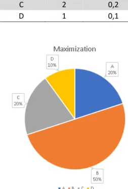
In Fitness Proportional Selection, or roulette wheel selection, the probability of an individual being selected is proportional to its fitness. The probability of selection on a maximization problem using fitness proportional is presented in Equation 3.

Equation 2 𝑃_𝑖 = 𝑓𝑖

∑𝑛−1𝑗=0𝑓𝑗

Table 2 and figure 9 show an example of the probability of selection by fitness proportional selection. Table 2 – Fitness proportional selection probabilities.

Individual Fitness Probability

A 2 0,2

B 5 0,5

C 2 0,2

D 1 0,1

Figure 9: Fitness proportional selection probabilities.

12

2.4.4.2.

Ranking Selection

In Ranking Selection, the probability of an individual being selected is the result of a function (example: a linear one) that determines the individual’s position in the selection queue. Equation 3 shows the formal probability of an individual being selected.

Equation 3 𝑃𝑖 =_{∑ i}n

j n-1 j=0

Depending on the individual's position in the queue, a probability is assigned to them. It is based on this that an individual is selected or not. This algorithm does not take into account how much better than the other an individual is; it only uses its position in the rank.

Example: n=3 so {i0, i1, i2} and f0 > f1 > f2 , the ranking selection procedure is as follows :

1. Order the individuals in the population (sort them) from the worst to the best according to their fitness.

2. The probability of selecting an individual is a function of the position it occupies on the ranking. (it can be a linear function, exponential and others).

3. Perform a roulette wheel selection using these probabilities to select the individual. Table 3 – Rank Selection order example

Rank Individual

1 I(2)

2 I(1)

3 I(0)

Using:

Equation 4 𝑃𝑖=_∑ 𝑛 _𝑖

𝑗 𝑛−1 𝑗=0

We have the probabilities presented in equation 5 and figure 10.

Equation 5 𝑃𝑖₍₀₎= 3

3 + 1 + 2 = 1

2 𝑃𝑖(1) = 2 3 + 1 + 2 =

1

3 𝑃𝑖(2) = 1 3 + 1 + 2 =

1 6

13

2.4.4.3.

Tournament Selection

Tournament selection consists of random selection with repetition, samples of the population are selected, and the n best individuals of them are select to the variation phase. The steps involved are:

1. Randomly select a small subset of elements, with repetition (an element can appear several times in the subset).

2. Select the best in the subset

3. Repeat n times where n is the size of the set.

The size of the tournament is a parameter, the bigger the subset, the higher the probability of choosing the best in the population.

• Big Tournament size implies big selection pressure. • Small Tournament size implies low selection pressure.

With this selection method, there is no need to calculate the fitness of all the individuals in the population, so it is less computationally intensive, only the individuals that are included in a tournament will have their fitness computed, this characteristic makes tournament selection a widely used selection method.

2.4.4.4.

Steady State Selection

Steady state selection, splits the population into blocks, grouping the individuals by their fitness, then, performs the variations on a subset of the best individuals, keeping the ones with the best fitness(Sivanandam & Deepa, 2008) and using the new offspring to replace the individuals with bad fitness, so that the new generation is composed of the best individuals and the new individuals evolved from the best.

This selection method is similar to many organisms in nature where in practice parents compete with their offspring, and strong individuals can outlive one or more generations.

2.4.4.5.

Reward Based Selection

This selection method chooses the individual not only by its fitness but also by combining with a cumulative reward given by all its parents.(Deb, Pratap, Agarwal, & Meyarivan, 2002)

14

2.4.5.

Variation phase and variation methods.

This phase will induce variations on individuals (simulating natural evolution), it is composed of crossover (cx), mutation (mx) and reproduction (the last does not change anything on an individual), any of these phases happen with a given probability defined on the algorithm parameters.

Figure 12: Variation phase.

2.4.5.1.

Crossover

Crossover is the combination of individuals, where two individuals exchange their genetic material with the intent of producing offspring that is better than any of them. Depending on the encoding being used there are different crossover methods, figure 12 shows binary crossover between two individuals.

In binary crossover, random positions on the genome are ‘marked’ (at least one position), then two new individuals are created by exchanging the parts delimited by these markers, between the two parents. This type of crossover should only be used with individuals where there is no need to keep any syntactical consistency.

15 There are more complex variations of crossover that are used when syntactical coherence is necessary or when it is not acceptable to lose any individual’s component into another individual, causing repetitions on one and omissions in the genome of the other. (example traveling salesman problem), one of these techniques, cycle crossover, avoids disrupting the individuals by using a cycle that only ends when it reaches a full loop through the individuals to be replaced.

Figure 14: Cycle crossover

Figure 14 shows an example of cycle-crossover on a representation of a traveling salesman problem7_,

note that in the offspring there is no omission or repetition of the cities represented by numbers.

2.4.5.2.

Mutation

Mutation is a change in the individual; this can be a simple binary mutation where one or more bits are swapped or a more complex mutation like Partial Inversion mutation

Figure 15: Binary mutation

Figure 16: Inversion mutation

More complex variations of mutations, like inversion mutation, are used when it is not acceptable to

lose an individual’s component (example traveling salesman problem)

2.4.5.3.

Reproduction

In reproduction, the offspring is an exact copy of the parents, i.e. no genetic operators are applied, and they are copied exactly as they are.

7 _{Common Computer Science scenario where we must choose the shortest path for a salesman to travel}

16

2.5.

C

G

P

.

GP consists of the use of genetic algorithms to evolve computer programs. On a more formal way, Poli writes in his book ‘A Field guide to Genetic Programming’(Poli, Langdon, & McPhee, 2008):

‘Genetic programming (GP) is an evolutionary computation (EC) technique that automatically solves problems without requiring the user to know or specify the form or structure of the solution in advance.

At the most abstract level GP is a systematic, domain-independent method for getting computers to solve problems automatically starting from a high-level statement of what needs to be done.’

A Common way to build the programs is by using a set of functions and terminal sets. Functions and terminal sets are dependent on the problem being solved. In regression problems, where mathematical expressions are created, the function set consists on mathematical functions like addition ‘+’ , subtraction ‘-‘,multiplication ‘*’ and division ‘/’8_{, the terminal set is composed of the}

input variables and constants.

Figure 17 presents the RPN representation of a genetic program to approximate the sin function, generated from a dataset containing the values of the sin from -5 to 5 in 0.1 increments, the solution has not been simplified and presents signs of bloat (see section 2.7.5.4). Figure 18 presents the plot of the function (result) and the data where the algorithm trained (target).

Figure 17: RPN representation of a solution.

Figure 18: Plot of a solution found to approximate the sin function.

In other problems like the Santa Fe Trail Ant problem9_{(Koza, 1992) the terminal set is a set of actions}

{Left, Right, Move}, and the function set is composed of a single function IfFoodAhead, these are arranged to control the movement of an artificial ant on a maze.

8 _{In genetic programming, there is a widespread practice to use safe division. Safe division protect the}

program from errors that would be generated by divisions by 0. Safe division can return different values depending on the objective, koza proposed(Koza, 1994) to return a 1, but other authors(Keijzer, 2003) use different approaches to avoid function approximation by use of asymptotes.

9 _{The santa fe trail problem(Koza, 1992), simulates an ant searching for food pallets laid on a}

17

2.5.1.

Classic Genetic Programming Algorithm.

GP employs genetic algorithms to produce individuals that are computer programs, so, like in genetic algorithms, in GP there are also the initialization, variation, and evaluation phases.

Classic GP Algorithm:

1 Create an initial population P of n random programs. (Initialization)

2. Repeat until the termination criteria are satisfied.

2.1. Calculate fitness of all individuals. (Except if using tournament selection)

2.2. Create an empty population P'. 2.3. Repeat until P' is filled.

2.3.1. Choose a genetic operator, (crossover with probability Pc, otherwise, reproduction with probability 1-Pc

2.3.2. Select two programs with a selection algorithm 2.3.3. Apply operator selected in 2.3.1 to the

individuals selected in 2.3.2.

2.3.4. Apply mutation to programs obtained in 2.3.3 with a probability of Pm.

2.3.5. Insert resulting individuals into P' 2.3.6. Iterate until P' contains n programs. 2.4. Replace P with P'

3. Return best program evolved.

Before starting the algorithm, we must:

1) Define a language to express the algorithm, example: RPN. 2) Select function set and terminal set if applicable.

3) Set the values of some parameters. 4) Define a fitness function.

2.5.2.

Program Representation

Programs can be represented in several forms, Koza (John R. Koza, n.d.; Koza, 1992) suggested the representation as trees due to the simplicity of implementation in computers using LISP10_{. Trees can}

be represented in a linear fashion too. Since in this case, I will be using polynomial expressions, the Reverse Polish Notation (RPN) also known as Postfix notation (these terms will be utilized interchangeably) will be employed and represented linearly.The infix notation (or algebraic notation) despite being the most common way to present mathematical expressions has the disadvantage of being more complex in computational terms, as it must be completely parsed before any evaluation can be performed, this arises from the different precedence that different operators have. RPN or Postfix eliminates the need for the interpreter to know the precedence of operators. RPN uses a stack based structure where operands are pushed first into the stack, and, an operator is applied to them in order. (Figure 19)

18 The three examples presented in Figure 19 show the same program or expression, in this case, a simple quadratic equation, represented in these three forms: tree graph, infix or algebraic and postfix or RPN notation.

The Graphic representation of the tree: Algebraic or infix notation:

𝑥2_{+ 2𝑥}

RPN or postfix notation:

𝑥 𝑥 ∗ 2 𝑥 ∗ +

Figure 19: Representation of an expression

How Postfix or RPN (Reverse Polish Notation) works:

RPN uses a list of elements to be evaluated; these elements are processed in order. When parsed, if the element is a number it is pushed to the stack, if it is an operand it pops the previously stacked element or elements and applies the operand to them, then, pushes the result onto the stack again, this process is repeated until there is nothing more to input, and only one value remains on the stack, this last value is the result.

Example:

Take the algebraic expression ((6+4)*5)/2, its RPN representation is 5 4 6 + * 2 /, and is evaluated as presented in table 4.

Table 4 – RPN processing example.

Input Type Stack Notes

5 Operand 5 Push 5 into the stack 4 Operand 5 4 Push 4 into the stack 6 Operand 5 4 6 Push 6 into the stack

+ Operator 5 10 Pop 6 and 4 from the stack, add, push the result into the stack * Operator 50 Pop 5 and 10, multiply and push the result into the stack. 2 Operand 50 2 Push 2 into the stack

19

2.5.3.

Common GP Parameters

To initialize the algorithm a set of parameters must be defined ‘a priori’, these are highly dependent on the problem being addressed, some of these parameters are:

• Population Size – Number of individuals that make up the population.

• Maximum number of generations – the number of generations to produce before terminating the program run.

• Selection Method – chooses the kind of selection that will be uses, examples, fitness proportional, tournament or others.

• Tournament size –This parameter sets the number of individuals that participate in the tournament.

• Crossover Probability (Px) – Probability for the crossover to occur, this value also implies the probability of reproduction to happen, as it is 1-Px.

• Mutation Probability (Pm ) – Probability of mutation.

• Mutation mode – Type of mutation to perform, point, subtree, etc.

• Elitism – If the best individual/Individuals of a previous generation are copied to the new generation.

• Initial Population generation mode – How the initial generation is created, full, grow or RHaH. • Initial population depth – The maximum ‘size’ of the individuals in the initial generation.

2.5.4.

GP Fitness evaluation

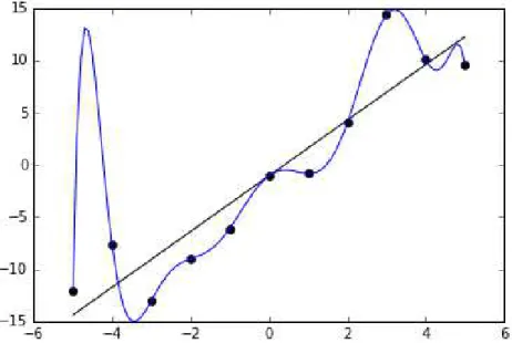
Intuitively, using figure 20, in a minimization problem, using distance as a fitness function, the smaller the area between the achieved result (blue), and the target result (orange) the fitter and better is the solution.

Figure 20: Representation of a solution to the sin function in different generations, left: early generation, right: late generation.

The fitness function used above is the minimization of RMSE(Vanneschi, 2014)(Zaji & Bonakdari, 2015) where the difference between the hypothesis presented by the individual and the data set result is calculated using equation 6.

Equation 6 _{𝐸 =} 1

𝑀√∑(𝑓(𝑥0, 𝑥1, 𝑥2, …

𝑀

𝑖=1

, 𝑥𝑖) − 𝑦𝑖)2

20

2.5.5.

Population Initialization and initialization methods.

The initial population is initialized at random. The initialization phase must produce individuals in the correct form for the problem being addressed, in other words, the individuals should be syntactically correct. If possible, the initial population should be as diverse as possible.

Initialization methods:

There are three main initialization algorithms to create the initial population, growth, full and ramped half and half.

Growth algorithm:

1) Create two sets, one with the Functions or operators (A) and one with the terminators or operands (B).

2) Define the tree depth D.

3) In tree depth 0 (the main node), randomly choose an operator from A. 4) Repeat until depth=D-1 or all branches are terminated with operands.

a. Select a random element from the set A U B. (a set of both operators and operands). 5) Terminate all branches that do not have an operand.

This method creates uneven trees, and the depth of the individuals is unpredictable.

Full algorithm:

1) Create two sets, one with the Functions or operators (A) and one with the terminators or operands (B).

2) Define the tree depth D.

3) In tree depth 0 (the main node), randomly choose an operator from A. 4) Repeat until depth=D-1.

a. Select a random element from the set A (a set with only operators). 5) Terminate all branches with an operand from set B.

This method creates trees that are always of the same size D; there are no simpler trees.

21

Ramped half and half

This algorithm addresses the problems of the previous two by creating an initial population that is generated using both growth and full algorithms and with different sizes, a population generated this way is more diverse in both size and structure.

1) Define how many trees we need to create. (population size)

2) Divide the population into D groups where D equals the maximum depth 3) Decide how many individuals we have in each group (Population size/D) 4) assign each group a maximum depth:

a. Group 1 - max depth = 1 b. Group 2 - max depth = 2 c. Group 3 - max depth = 3 d. …

e. Group D - max depth = D

5) For each group, half of the individuals will be generated with the growth algorithm and the other half with the full algorithm using the corresponding maximum depth.

2.5.6.

Selection Phase

In GP the selection methods do not differ much from the ones in Genetic algorithms. The only difference is in the fitness function that is applied. Due to the computational cost of evaluating the fitness of a Genetic Program, tournament selection is widely used in this phase avoiding the task of evaluating every individual in the population.

2.5.7.

Variation Phase (Crossover and Mutation)

Variation techniques in GP must preserve the correct syntax of the program being created so that it still makes syntactical sense after the mutation or crossover.

2.5.7.1.

Mutation

For mutation, a random node is selected from the tree, then depending on the method, that node is replaced with another from the same set (operators/operands) or a new sub-tree is grown starting on that node. Care must be taken to preserve syntactical coherence.

Figure 22: Mutation Example, left: the original tree, middle: point mutation and right: sub-tree

22

2.5.7.2.

Crossover

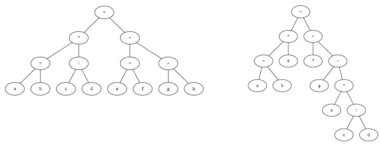
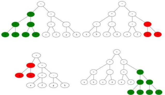
Like in GA, crossover takes parts from both parents and combines them into new individuals. When performing a crossover, a node is selected in each of the parents, then, that node and all its siblings are cut out and swapped from one parent to the other. This important part is that the whole functional part is exchanged so that the RPN evaluation can be completed successfully. The syntax of the program must be maintained.

Figure 23: Crossover Example, above two parents, the selected part is in red and green, below, the siblings with the swapped parts still in their parent’s color.

2.5.7.3.

Reproduction

Like in G.A. in reproduction the offspring is an exact copy of the parents without the application of any genetic operators.

2.5.7.4.

Bloat

23

2.6.

R

B

G

P

.

In this thesis, we extend classic GP with the use of repulsors. This section will set the ground for the repulsor based approach used in this dissertation.

2.6.1.

Repulsors.

A repulsor is an individual that has some trait that caused him to overfit in a set that was not directly used in training, in this case, a validation set. The repulsors as they are found (through overfit detection) are placed on a repulsor list.

2.6.2.

Overfit detection.

Overfit detection signals individuals as overfitters if they meet some predetermined criteria, the criteria is dependent on the approach. In the case of this dissertation we use the difference in fitness from the previous generation, see section 6.6 for details.

2.6.3.

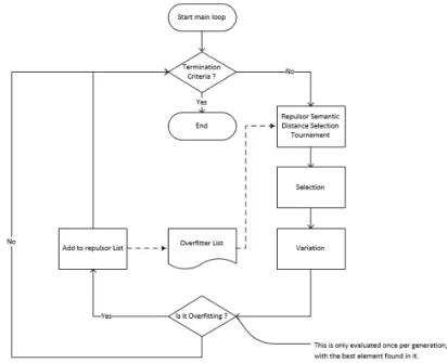
GP Repulsors Algorithm.

The algorithm is an extension of GP Classic with the inclusion of the overfit detection and the additional repulsor based selection phase. Where we select the individuals based on their semantic distance from the repulsor list. The further the solution is from the individuals in the list, the better.

So, the fittest individuals, will perform well in the standard selection with the standard fitness function (usually minimizing the difference), and will also perform well in the repulsor tournament (usually maximizing the difference between themselves and the repulsors).

Figure 24: Repulsor based algorithm example.