The Determinants of
Non-residential Real Estate
Values with Special
Reference to Local
Environmental Goods
Sofia F. Franco
W. Bowman Cutter
Working Paper
# 603
2016
1
The Determinants of Non-residential Real Estate Values with Special Reference to Local Environmental Goods
Sofia F. Franco1 W. Bowman Cutter2
May 10th 2016
Abstract
This paper presents the results of an empirical study of the determinants of non-residential real estate values in Los Angeles County. The data base consists of 13, 370 property transactions from 1996 to 2005. Separate spatial econometric models are developed for industrial, commercial, retail and office properties. The study focus on the impact on property values of local amenities.
Our analytical results provide insights on how amenities may affect non-residential properties values and how the impact may differ across property types. Our empirical results offer evidence that explicitly modeling spatial dependence is necessary for hedonic non-residential property models where there is interest in local amenities. We also show that it is also important to account for the temporal dimension since ignoring it can lead to misinterpretation of the real measure of spatial dependence over time. Moreover, we find that in general amenities that are jointly valuable to firms and household, such as parks or air quality have either weak or non-robust effects on nonresidential values. However, the fact that the joint amenities coastal access and crime appear to have stable correlations across specifications would be consistent with a higher firm than household valuation. In contrast, those amenities that are likely only valued by firms, such as transportation access and proximity to concentrations of skilled workers have robust and significant correlations with non-residential values.
JEL Codes: R52, H23.
Keywords: Non-residential Property Values, Local Environmental Amenities, Spatial Econometrics
1 Corresponding Author. Universidade Nova de Lisboa, Nova School of Business and Economics (NovaSBE)
and UECE- Research Unit on Complexity and Economics, ISEG-UTL, Lisboa, Portugal Address: Nova School of Business and Economics, Campus de Campolide,1099-032, Lisboa, Portugal. Email [email protected]. Phone Number: + (351) 213801600. Dr. Franco greatly acknowledges the financial support by FCT (Fundação para a
Ciência e a Tecnologia), Portugal. This article is part of project PTDC/IIM-ECO/4546/2014.
2Pomona College, Department of Economics, Claremont, CA 91711; Telephone 909-607-8187; Email
2 1. Introduction
The economic literature has exhaustively studied the influence on housing prices of environmental goods including air quality (Bayer et al. 2009, Kim et al. 2003, Chay and Greenstone 2005, Bockstael and McConnell 2007), views (Rodriguez and Sirmans 1994, Seiler et al. 2001, Bond et al. 2002), crime (Pope 2008, Grove 2008), urban forests (Tyrvainem and Miettinen 2000, Mansfield et al. 2005), water quality (Leggett and Bockstael 2000), proximity to hazards (Bin and Polasky 2004), and many other factors. By decomposing residential prices into their relevant components, this literature is able to reveal the amount by which households value the environmental amenities and disamenities being studied.
The commercial real estate sector is also a large part of the national economy, with an estimated $11 trillion value as of the end of 2009 (Florance et al. 2010). However, there are very few studies that have estimated the influence of amenities or disamenities on the value of non-residential properties. This is quite surprising because it is likely that these two markets are strongly linked. Offices, commercial and industrial properties compete for space with residential properties, and the wages firms can offer are influenced by this competition. Diamond (2012) suggests that firms seek to locate in metropolitan areas that have high concentrations of skilled workers. If that is a factor driving inter-metropolitan firm location, should it also not be a factor driving intra-metropolitan migration?
Moreover, temperature, humidity, wind, cloud cover and precipitation also determine how much energy it takes to keep interior spaces lit and at comfortable temperatures and therefore, impact firms’ cost structure. If in fact, firms observe and capitalize these types of amenities, hedonic methods can be used to measure the price premium for such attributes, representing the valuation of the marginal buyer. However, it is unclear how these amenities will be valued in equilibrium where both firms and households compete for desirable locations. One goal of this paper is to develop such a model.
While there is already valuable work that identifies appropriate environmental indicators for built non-residential assets, these studies focus on the design and building construction (see for example Eichholtz et al. 2013) and lesser consideration has been given to the impacts of local public goods such as crime, presence of skilled workers, weather, air pollution or alternative forms of open space on rents and selling prices of non-residential properties.
The goal of this paper is therefore to understand how non-residential property values correlate to local amenities using data on office, commercial, industrial and retail property sales from Los Angeles County.
The theoretical urban equilibrium model we develop shows that amenities that influence either commercial or residential property prices will influence the prices and development of both types of property. In addition, it provides a rigorous theoretical foundation for variable choice and for the control
3
of spatial and temporal dependence in properties valuations in our empirical model of non-residential property prices.
The empirical portion of this paper seeks to test the predictions of the theoretical model by measuring how key neighborhood or geographical characteristics are related to non-residential property prices. In addition, it also investigates whether spatial and temporal dependences should be accounted for in all sub-sectors of the non-residential market, namely retail, office and industrial. Spatial dependence implies that high (low) priced real estate assets tend to cluster in some locations (Anselin and Bera 1998).3 This is particular relevant since not accounting for spatial autocorrelation (or spatial dependence)
in presence of spatial interactions in the non-residential real estate market may lead to mispricing of not only building attributes but also of local amenities. The degree of cross section dependence is usually calibrated by means of a weighting matrix, where weights can be based on alternatives forms of contiguity, distance, square distance or the number of nearest neighbors. The spatial weight matrix captures how two properties are spatially connected to one another at one point in time. However, the values for each property are also likely to be correlated with each other over time.
While it is likely that spatially close past property values influence current property values, it is unlikely that spatially close future and unknown property values influence present values. Therefore, the spatial weights matrix needs to be adjusted for potential temporal influence on the spatial spillover impacts in a temporal context. Ignoring such temporal dimension in constructing the weights matrix could lead to misinterpretations on the real measure of spatial dependence over time, which in turn has implications for the influence of local amenities on property values (Dube and Legros 2013, 2015).
We first run a hedonic model as a benchmark against which we will compare the subsequent model specifications. Then we employ spatial econometric models that employ spatial and spatio-temporal weights matrices. These models are applied to 13, 370 non-residential property transactions in Los Angeles County from 1996 to 2005. Given its multimodal structure, heterogeneity across nodes, surrounding jurisdictions and environmental amenities, Los Angeles County provides an appropriate spatial setting to illustrate the theory developed in our theoretical session.
Sivitanidou (1995) and Sivitanidou and Sivitanides (1995) are the most complete papers in the non-residential rents literature. These papers include a number of geographic and workforce attributes. However, the less-advanced geographical software of the time did not allow those authors to be as
3 In real estate markets, due to herd behavior of buyers and sellers, the value of a property generally guides price
expectations in a neighborhood (Hott and Monnin 2008, Hott 2012). Furthermore, neighborhoods tend to develop at the same time and may have similar structural characteristics, such as dwelling size, vintage, interior and exterior design features (Basu and Thibodeau 1998). Nearby buildings tend also to share the same local amenities like accessibility, environmental characteristics, and have similar access to labor markets and public facilities.
4
geographically specific as our paper. In addition, we include many green and infrastructure amenities that those authors likely lacked. Finally, we use a spatial econometric estimator to capture spatial correlation in both the dependent variable (property prices) as well as in unobservables (residuals). We also construct a spatio-temporal weights matrix, following Dube and Legros (2013, 2015) methodology, to evaluate spatial dependence in a context of spatial data (cross-section) pooled over time.4
The sources of non-residential real estate value are interesting in their own right, but our research also sheds light on the literature on quality of life and intra-city productivity divergence. The current work on quality of life and city productivity divergence (Diamond 2012, Albouy 2012) tends to assume that metropolitan areas (MSAs) are spatially uniform and stresses differences between MSAs. However, MSAs can be quite large and there is likely to be significant intra-MSA differences in productivity and quality of life. Diamond 2012, especially, posits a dynamic cycle where skill agglomeration increases productivity, attracting business, which attracts more skilled employees and increases productivity further. Also, the critical mass of skilled employees creates a market for shopping and entertainment that also draws more skilled workers. This story contains the hypothesis that firms should locate near concentrations of skilled workers, which we test in the empirical portion of our paper. We also test whether firms value proximity to restaurants and shopping.
Our empirical results indicate the importance of controlling for spatial dependence in estimating the determinants of non-residential values. Spatial parameters are generally statistically significant, and our simulations indicate that non-spatial estimates of amenity elasticities vary from those generated by spatial regressions. However, similar to Dube and Legros (2013, 2015), we also find that ignoring the temporal dimension in constructing the weights matrix leads to misinterpretations on the real measure of spatial dependence over time. In particular, our results suggest that, for the Los Angeles market, accounting for spatial-temporal dependence in the lagged dependent variable (sale prices), does not seem to attenuate the effects of hedonic attributes statistically or economically.
Regarding the impacts of local amenities, we find that in general amenities that are jointly valuable to firms and household, such as parks or air quality have either weak or robust effects on non-residential values. However, the fact that the joint amenities coastal access and crime appear to have
4 Note that panel data consists of the same unit observed over time, while pooled cross-section data consists of a
different unit observed over time, so that a unit is only observed once or very infrequently. Spatial, or cross-sectional, databases pooled over time can represent for example real estate sale prices, business opening (or)/closings, crime location or innovation. For these databases, the panel procedures cannot be applied because a given spatial observation (located at a point) is only observed once over time. However, Dube and Legros (2013, 2015) clearly show that neglecting the temporal dimension of the data generating process of spatial data pooled over time can generate biases on the autoregressive coefficient as well as on the coefficient related to the independent variable which can lead to erroneous interpretation of the indirect and total marginal effect related to spatial characterization.
5
stable correlations across specifications would be consistent with a higher firm than household valuation. In contrast, those amenities that are likely only valued by firms, such as transportation access and proximity to concentrations of skilled workers have robust and significant correlations with non-residential values. Our results are thus aligned with those of Gabriel and Rosenthal (2004), suggesting that households and firms value differently local amenities. For this reason, cities or MSAs that are attractive to firms may be unattractive to households, and vice-versa.
We begin the remaining portion of our paper by examining the literature concerning the determinants of non-residential rents and values and the related quality of life and quality of the business environment literature. In section 3 we develop a model of the joint determination of non-residential and residential rents and values that include the role of amenities and herding behavior by the market participants followed by comparative static analysis in section 4. Section 5 describes the empirical framework and the econometric model of non-residential values that includes amenities and spatial and temporal dependences and auto-correlation. It also discusses the data, which represents a unique combination of non-residential property transaction data with detailed information on building attributes and local natural and man-made environmental and urban amenities. Section 6 provides the main empirical results and finally, section 7 offers conclusions.
2. Literature Review
Application of the hedonic method to the non-residential property (office, commercial, office) market is recent compared to the housing market and, as a result, references are much fewer. This is primarily explained by the difficulty of collecting the necessary databases, as description of properties by their characteristics is generally less reliable for retail, office-commercial and industrial real estate and warehouses than for housing. However, the improvement in information quality since the 1990s has encouraged development of this type of work, which for the time being still covers only a limited number of geographical markets and has focused mostly on office-commercial real estate properties.
The most comprehensive studies of urban spatial variations in non-residential rents are by Sivitanidou (1995) and Sivitanidou and Sivitanides (1995). Both studies provide a framework for empirically analyzing location demand and supply-side influences on non-residential rents within multimodal MSAs. Coupled with a set of firm amenities reflecting traditional demand-side influences (access to CBD, freeway and airport) and a set of worker amenities (education, crime, access to shopping opportunities and distance to the ocean), supply-side factors such as local institutional controls were found in Sivitanidou (1995) to play an important role in shaping variations across space in office-commercial rents in Greater Los Angeles. A similar conclusion was also reached in Sivitanidou and Sivitanides (1995). In particular, the study concluded that although firm amenities induced the strongest
6
price effect, worker amenities and zoning constraints also played an important role in industrial pricing in Greater Los Angeles. While these studies provide important insights of the role these factors play in shaping intra-urban variations in business rents, they lack hedonic spatial techniques in their estimations and therefore, do not account for spatial heterogeneity and spatial autocorrelation.
In general, existing empirical studies on the determinants of office-commercial rents have provided consistent results on the contribution of various locational (distance from city center or distance from nearest highway interchange) and structural (such as total building square feet, age, height, occupancy, parking) variables to the spatial variation of office rents. Examples include Brennan et al. (1984) and Mills (1992) for Chicago, Sivitanidou (1995) for Los Angeles, Bollinger et al. (1998) for Atlanta, Dunse and Jones (1998) on the market in Glasgow and Nagai et al. (2000) for central Tokyo.
Some studies focus on a specific aspect of rent determinants: architectural features of the buildings (Doiron et al. 1992, Hough and Kratz 1983), vacancy rate (Frew and Jud 1988; Wheaton and Torto 1988; Sivitanides 1997), access to main and secondary CBD centers (Bollinger et al. 1998, Sivitanidou 1995), or proximity to light rail transit and highway systems (Ryan 2005). More recently, studies have measured the effect of environmental certification on office-commercial (Eichholtz et al. 2010, Miller et al. 2008, Fuerst and McAllister 2011a,b,c) and industrial warehouse (Harrison and Seiler 2011) rents. Recognition of the adverse effects of urban sprawl and a heightened awareness of environmental concerns has contributed to the growth of the green building design and construction movement in the United States. Yet, none of the previous studies have examined the relative contribution of urban green spaces and environmental quality (such as levels of air pollution) to the spatial variation in non-residential rents within multimodal metropolises. It is nevertheless possible that the observed ripple effect of nearby open space, landscape scenery and air pollution on residential properties may also apply to retail and office sites.
The hedonic price approach has long been used to quantify the impact of open space on residential property value, including urban parks and golf courses (Bolitzer and Netusil 2000, Lutzenhiser and Netusil 2001). A common finding in these studies is that green spaces of these types have positive impacts on residential property values up to a distance of one-quarter to one-half mile. As much as 3% of the value of properties could be attributed to park proximity, while proximity to golf courses increased surrounding property values as much as 21%. There is also empirical evidence that increasing the amount of water and grassy land covers in views result in increased home sale prices (Sander and Polasky 2009). For a review on published articles that have attempted to estimate the value of different types of open space see McConnell and Walls (2005). Bockstael and McConnell (2007), in a review of wage studies, also find clear evidence that households are willing to give up wages to live in cleaner
7
locations. Thus higher residential rents and lower wages do not represent a higher “cost of living” in the nice locations but rather a higher “benefit of living” there.
In fact, when amenities have little or no effect on firm costs, either real-estate prices or incomes can be used as an indicator of quality of life from the households’ point of view. Several studies have computed quality-of-life rankings for cities, urban counties and metropolitan areas by running two hedonic equations: one relating housing prices to different amenity variables (such as precipitation, temperature measures, sunshine, coastal access, crime, air and water pollution) as well as to housing characteristics; and the other relating incomes for individual households to the amenity levels and workers’ characteristics. Examples of such studies include Hoehn et al (1987), Blomquist et al. (1988), Gabriel and Rosenthal (2004), Albouy (2012). However, since the connections between quality of life and real-estate prices and incomes can be ambiguous when firms costs are strongly linked to amenities, neither of these variables can be generally used with confidence as an unambiguous indicator of quality of life. Given all the interdependencies between amenities and households, firms and real-estate developers decisions, it is possible that both hedonic price and wage regressions yield reverse results even if these effects are theoretical possible.5
On the other hand, since amenities also affect firms, the empirical procedure used in quality-of-life studies can also be used to rank cities, counties or metropolitan areas from the perspective of firms. For example, Rosenthal and Gabriel (2004) have performed an empirical exercise similar to the procedure used in papers generating quality-of-life rankings. Their study found that the ranking of cities by firms is very different from the ranking by households, consistent with the different goals of the two groups, suggesting that the effects of amenities on consumer utilities and firm profits are often not in the same direction. This in turn suggests that firms and households may also not value environmental amenities and/or environmental quality the same way. Yet, no studies so far have examined the impact of alternative environmental amenities and environmental quality on non-residential real estate values and rents.
3. The Model
This section develops the theoretical underpinnings of the paper. Our framework builds on the model developed by Sivitanidou (1995) and Hott (2012) in order to analyze the effects of local amenities on
5 For example, in the housing-price regression of Blomquist et al. (1988), better public safety leads to lower rather
than higher housing prices and in the hedonic wage regression higher particulate pollution reduces rather than increases income.
8
non-residential real estate values.6 By accounting for firm, worker, floor-space and land market
equilibriums, our modeling scheme justifies the inclusion in the non-residential hedonic price function of not only productivity-enhancing firm amenities, but also utility-bearing worker amenities and land supply restrictions. In addition, by accounting for herd behavior of the market participants in the sense that the value of a property generally signals or guides price expectations in a neighborhood, our theoretical model justifies the inclusion of a spatial lag in our model specification. Finally, because neighborhood and accessibility attributes of a property are not always directly observable and sources of spatial autocorrelation in property prices also include measurement errors, unsuitable functional form and model misspecification, spatially correlated errors in hedonic model may result, which in turn require a specific statistical approach.
3.1. Assumptions
Let’s assume our county contains many cities, indexed by j. Cities differ in two types of attributes: natural and artificial amenities and land-use regulations.
Some amenities (e.g. costal proximity) directly affect households’ utility, while others (good transportation access facilitating trips within or out of the city or agglomeration economies) directly affect firms’ productivity or transportation costs. Other amenities (e.g. climate conditions and public safety) may affect both the location of firms and households. Let A represent a vector of amenities in Hj
city j that directly affect households’ utility and A is a vector of amenities in city Fj j affecting firms’ productivity and production.
Each city has two zoning methods to control land use: a restriction on the quantity of land available for a certain use and a set of regulations on office-commercial construction.
Land within each city is homogenous. Capital is costless mobile across cities, and is paid the price
i everywhere. Office-floor space is owned by absentee landlords who rent the space to local firms. Land is owned by absentee landowners who rent the land to local residents and local developers. Households are perfectly mobile, have identical tastes and skills, and each supply a single unit of labor. Office-commercial firms are also perfectly mobile and identical. All factors are fully employed and both output and input markets are competitive.
A long-run equilibrium requires that land, labor, and floor space markets be cleared simultaneously through appropriate rent and wage adjustments. Residential land rents (P ), office-commercial land Hj
6Hott (2012) model takes into account that a house can be seen as an asset which price should reflect a risk-return
9
rents (P ), firm floor space rents (Fj R ), labor wages (Fj w ), number of households/workers demanded j by each firm (N ) and number of firms (j F ), are endogenous. The equilibrium conditions in the model’s j
various markets are discussed below.
3.2. Households Equilibrium
Households have preferences over residential land, h, a numeraire nonland good, z, and a set of households’ amenitiesA .Hj 7 At each city, a household solves the following utility maximization
problem: 0 , . . ) , ( max ) ; , ( w w z h P t s A z h U A P w V j Hj Hj z h Hj Hj j (1)
where U()is concave over h and z and increasing in A , Hj P is the rental expenses on residential Hj land per unit of land andw is wage in city j j. The nonlabor income w0 is assumed to be independent of location and will be suppressed in the model henceforth. For simplicity, we assume that the price of the numeraire good is set to 1. The solution of (1) yields the demand functions for residential land and the nonhousing good as
) , ( j Hj d P w h (2) ) (wj z (3) where wd 0 j h , Pd 0 Hj h .8
The indirect utility function V(wj,PHj;AHj)gives the maximum utility achieved in city j given the wage, the residential land price and the level of households’ amenities. Households choose residential locations to maximize V(wj,PHj;AHj) by considering the trade-offs between wage, residential land rents and households’ amenities. Since households are fully mobile, their utility must be the same across all the cities that they inhabit. Therefore, equilibrium for households requires that wages and residential land rents adjust to equalize utility in all cities:
V A P w A P w V( j, Hj; Hj)( j, Hj) Hj (4)
7 Spatial variations in nonhousing costs, which are smaller than spatial variations in housing costs, are ignored in
this analysis.
8 Note that because
Hj
A is separable in the utility function, (2) and (3) do not depend directly on the city’s households’ amenities.
10
where V is the exogenous uniform utility level and (.) is a function that satisfies wj 0 and 0
Hj P . Therefore, Vwj 0, 0 Hj A V and 0 Hj P V .
If there are NSj households/workers in city j, then total demand for residential land is given by ) , ( j Hj d S jh w P N . (5)
3.3. Office-Commercial Firms Equilibrium
Office-Commercial firms produce output with a constant returns production function involving the use of office-commercial space (S ) and labor (j N ). In addition, the production function in city j j
incorporates external effects represented by a Hicks-neutral technical change A . Output is exported at Fj a uniform exogenous price, which we set equal to 1. At any given city, a firm takes as given input prices and production amenities and chooses the best combination of labor and office-commercial space to minimize the total production cost:
Q S N Q A t s S R N w A R w C j j Fj j j j j S N Fj j j j j ) , ( . . min ) ; , ( , (6)
where Q is the optimal output (which is determined by the production technologies and markets and is set before the location decision is made) and R is the rental price of one unit of office-commercial j
floor space. The solution to (6) gives the firm’s conditional demands for labor and office-commercial space in cityjas:
) , ; , ( j j Fj d j w R Q A N (7) ) , ; , ( j j Fj j w R Q A S (8) where Ndj /wj 0, Ndj /Rj 0, Ndj /AFj0, Sj/wj 0,Sj/Rj 0and Sj/AFj 0. Under Hicks-neutral technical change, it is clear that Sdj(wj,Rj;Q,AFj)/Ndj(wj,Rj;Q,AFj) is independent of the A . Because Q is assumed to be independent of location, for simplicity it is Fj
henceforth assumed to be equal to 1. Equilibrium for firms requires that wages and office-commercial rents adjust to equalize costs in all cities:
C A R w
11
where C is a constant determined by the existing production technologies. Moreover, because we assume A to be Hicks-neutral and firms produce output under constant returns to scale, the cost Fj
function in equation (9) can be written as Fj j j Fj j j R A w R A w C( , ; )( , )/ (10) where 0 j w and 0 j R . Therefore, Cwj 0, 0 j R C and 0 Fj A C . Equation (10) is a downward
sloping function in the (wj,Rj) space, that is, 0
j j
dw dR
. This means that for a given level of firm amenities, locations with higher labor costs must have lower rental cost to equalize total cost across locations. In addition, since production has constant returns to scale, the unit cost of production (which is independent of the output level) equals the exogenous output price and as a result any non-negative output level is a solution to the profit maximization problem and generates zero profits.
Let F represent the number of office-commercial firms in city j j. Then total demand for office-commercial floor space in city j is given by
) , 1 ; , ( j j Fj j jS w R A F . (11)
3.4. The Office-Commercial Floor-Space Market
The office-commercial floor-space is a competitive industry, with profits at all locations equal to zero. Real estate developers supply office-commercial space under constant returns using capital and land. The production process may be subject to institutional constraints (for example impact fees or difficulties in obtaining building permits), which enter the production function as a Hicks neutral shift parameter. Based on profit optimization and given constant returns, long-run equilibrium in the office-commercial floor space market is ensured by equating the unit rental price of floor space (given by the LHS in (12)) to unit production costs (given by the RHS in (12)), as indicated by
j Fj j i P G
R (, ) (12) where () is an increasing function in both input prices. P is the endogenous price for office-Fj commercial land and G is a vector of institutional constrains on office-commercial construction such j
that Gj 1. Note that a Gj 1increases office-commercial construction costs. Moreover, equation (12) implicitly defines the land bid-rent of office-commercial floor-space producers as the price of land such that profits are zero. In order not to introduce further structure to the model, we assume that the number of real estate developers in city j is fixed and normalized to one.
12 3.5 The Land Market
To ensure equilibrium in the land market, P and Fj P must be such that total land demanded by Hj real estate developers and by households equals the fixed supply of land available for each use, as shown by Fj Fj j j j Fj D P w R F A i L L ( , , ; , , ) (13) Hj Hj j d Fj j j d j jN w R A h w P L F ( , ,1; ) ( , ) (14) where LFjand LHjrepresent the total amount of land available in city j for office-commercial and residential land use, respectively. Since the production function for office-commercial space has constant returns to scale, then total demand for office-commercial land can be expressed as
) , ( ) , 1 , , ( ) , , ; , , ( Fj j j j Fj j j j Fj Fj D P w R F A i F S w R A i P L (15) where i 0 and 0 Fj P
. Note that in equilibrium total supply of office-commercial floor-space must satisfy total demand for office-commercial space in city j, which is given by (11). Therefore,
) , 1 ; , ( j j Fj jS w R A
F should be the optimal amount produced and supplied in cityj by real estate developers.
In addition, equilibrium condition (14) implies that the labor market must also be in equilibrium. From (7), each office-commercial firm in city j demands Ndj(wj,Rj;1,AFj)units of labor. Since there are F firms in cityj j, total demand for labor is given byFjNdj(w,Rj,1,AF). Because we assume there is full employment and households live where they work, then t
otal demand for labor in cityjequals the total number of households living in the city. From (2), a household living in city j demands hd(wj,PHj) units of residential land. Therefore, the LHS of (14) is the total demand for residential land in city
j
.3.6. Office-Commercial Rent (and Wages) Equilibrium
Given the exogenous parameters of the model, equations (4), (9), (12)-(15) and (7)-(8) should determine unique equilibrium values for the model’s simultaneously determined endogenous variables
Fj
P , P , Hj R , j w and j F . j
Equation (14) implicitly determines P as a function of (Hj wj,Fj,Ndj,LHj). Note that the cost of
13
of firms and total amount of land available for office-commercial use. Inserting PHj(wj,Fj,Ndj,LHj) and (7) into (4) while taking into account (12) , (13) , that the office production function has constant returns to scale and that firm’s amenities enter the production function a la Hicks, yields the modified household equilibrium condition
V A i G L L R P w V( j, Hj( j, Hj, Fj, j, ,1), Hj) (16) where PHj/Rj 0, PHj/LHj 0,PHj/LFj 0and PHj/Gj 0. Equation (16) is upward
sloping in the (wj,Rj) space, that is, 0
j j
dw dR
implying that for a given level of household amenities, locations that offer higher wages must also have higher office-commercial rents and higher housing residential land prices to equalize utility in all locations.
Equation (16) and equation (9) together jointly determine the equilibrium office-commercial rent and the equilibrium wage in city j as
) , , , , ( Fj Hj j Hj Fj j A A G L L R (17) ) , , , , ( Fj Hj j Hj Fj j A A G L L w (18) Omitting the spatially invariable parameters, the reduced-form office-commercial rent function (17) suggests that long-run office-commercial space rents must be a function of firm production amenities, household/worker amenities, legal restrictions on the production of office-commercial space, as well as land supply influences.
3.7. Office-Commercial Property Prices
From Rental Prices to Property Prices
If the property market works in accordance with conventional economic theory then the price of a property should be such that buyers are indifferent between renting and owing. Note however that rents are determined in the property market for space use, not in the asset market for ownership. Equation (17) captures thus the fundamental forces driving office-commercial rents and represents a central piece in determining the demand for real estate assets. The reason is because when investors acquire an asset (real estate property), they are actually acquiring a current or future income stream. Thus, in a frictionless market, rent should cover the user cost of a property, that is, the costs that arise from owing a property for one period:
( )
) , , , , ( , , , , , , 1 ,t Fjt Hjt jt Hjt Fjt jt t t t j A A G L L P i m E G R (19)14
wherePj,t is the property price
j
at time t , it is the real interest rate, m is the constant maintenance rate and Et(Gt1)is the expected capital gains defined ast j t j t j t t t P P P E d G E , , 1 , 1 ] ) ( ) 1 [( ) ( (20)
where d is the constant depreciation rate.
Inserting (20) into (19) yields, after some manipulations, the following property price equation:
m i P E d R P t t j t t j t j 1 ) ( ) 1 ( , 1 , , . (21) Herding Behavior
We now introduce herding behavior by assuming that rational but imperfectly informed investors learn from the decisions of the other investors. In particular, let’s assume that investor j expectations regarding the future property price depends on both social and non-social signals. Informational influence affects expectations of real estate price appreciation if investors look to others in deciding whether or not their real estate purchase will generate capital appreciation. In this sense, we can write the expectation regarding future price as Et(Pj,t1j), with representing the information set upon j which investor j bases his expected capital gains and described as follows:
t j j Q q Q q j q j x , P , 1 1 ,
(22) where q,j and Q,j are the weights placed by investor j on the information contained in the non-socialsignal x and social signal q Pj,t , respectively. It is assumed that 0q,j 1, q and 1
1 ,
Q q j q .According to (22) the information set has two different components. The first component on the right-hand-side of (22) captures all currently available objective information relating to non-social factors (x ) such as for example maintenance rate, depreciation rate and interest rates. q
The second component on the right-hand-side of (22) contains the social information regarding the willingness to pay of other owner occupiers for similar properties (xQ Pj,t). In this sense, our model captures the idea that a selling price of a property at a particular location acts as a signal that guides the selling prices of its neighboring properties.
15
If markets are weakly efficient, social signals are ignored (that is Q0for all investors) and all investors respond symmetrically to non-social signals so that q is constant across all investors, then the non-social information is factored into prices to give an unbiased estimate of future prices (Pt). In this case the expectation of future price is represented as
t Q q q q j t j t P x P E
) ( 1 1 1 , (23)However, when Q0, social information will distort prices away from their fundamental value. The action of other investors introduces herd externalities in which the herd’s judgment is biased by social information about the action of others:
t j Q t Q Q q q q j t j t P x P P E , 1 1 , ) (1 ) (
. (24) Representative office-commercial property price for cityj
at time tFinally, inserting (24) back into (21) we get the representative office-commercial property price for city
j
at time t as ] ) 1 [( 1 ) 1 ( 1 1 ] ) 1 )[( 1 ( , , , , , t j Q t Q t t t j t t j Q t Q t j t j P P m i d m i R m i P P d R P (25)with the fundamental value of office-commercial rents,Rj,t, given by equation (17). According to (25) real estate prices can divert from their fundamental value because of a herding behavior. The fundamental value of office-commercial properties is represented by:
m i R E m i d m i R P m i d m i R t t j t t t t j t t t t j 1 1 , , , 1 1 ) 1 ( 1 1 ) 1 ( 1 . (26)
Following (26), the fundamental price of a non-residential real estate property is driven by present and future office-commercial rents and interest rates. However, the presence of a herding behavior (
0 Q
) may create a positive feedback effect between the attractiveness of a real estate property and its price, Q[Pj,tPt]. If [Pj,tPt] is positive then the excess return from this price externality is positive, which pushes the price of a real estate property higher. On the other hand if [Pj,t Pt] is negative, the opposite effect occurs. The parameter Q captures the strength of price externality. This
16
in turn suggests that real estate markets are not fully efficient and autocorrelation in price inflation should be accounted for in studies that examine the determinants of real estate prices.
It is worth pointing out that [Pj,t Pt] captures proximity both in space and time because the social signal Pj,t incorporates property prices from spatial neighbors, which in turn incorporate expectations over future prices.
Equation (25) therefore sets the stage for the empirical analysis of office-commercial property values and location desirability within Los Angeles County. In section 5.3 we provide details on how we build our spatio-temporal weights matrix, which specifies the weight by using both the space and time of the nearest similar transacted property (neighbor). Each row in this matrix pertains to a transaction in our data set.
4. Comparative Statics
The equilibrium effects of land-use regulations, as well as production and household amenities, can be derived by totally differentiating (4), (9), (12)-(15) and (7)-(8) with respect to each variable of interest. Because of all the interdependencies, the comparative statics of this type of model can be fairly complex and lengthy. The steps for the case where the amenity is beneficial to households but neutral to firms are shown in the appendix, and the remaining derivations are available on request. In this section, we just indicate the signs for changes in each exogenous variable and discuss the results.
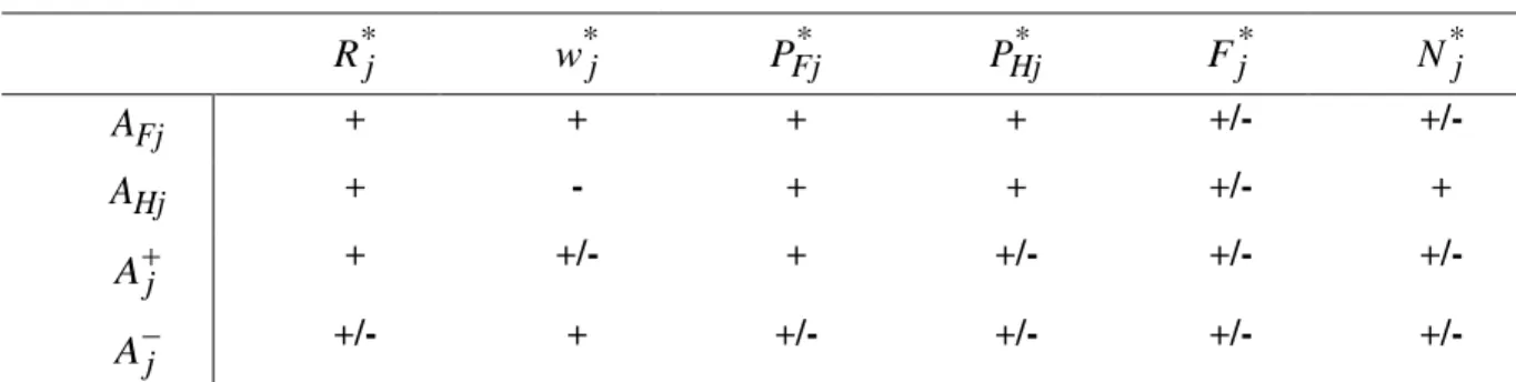
Table 1: Comparative Statics: Amenities
* j R w*j PFj* PHj* F*j N*j Fj
A
+ + + + +/- +/- HjA
+ - + + +/- + j A + +/- + +/- +/- +/- j A +/- + +/- +/- +/- +/-Note: A “+” ( “-”) indicates that the sign if the derivative is positive (negative). A “+/-” indicates that the sign of the derivative may be positive or negative.
Impact of an increase in office-commercial firm amenities (A ) Fj
For a given level of household amenities and land-use regulations, if firm amenities at cityj
increase, then office-commercial firms in the city must pay higher both for office-commercial rents and labor; otherwise, firms would have incentives to move to that location. On the other hand, households are willing to trade a higher wage for a higher residential land price in order to equalize utility across
17
cities. In addition, higher office-commercial land prices are established in city j, as more firms bid higher floor-space rents. However, higher labor and rental costs together with higher productivity have an ambiguous effect on the number of demanded workers and on the amount of demanded floor space. As a result, the impact of a change in firms’ amenities on the equilibrium number of workers/households in city j is ambiguous.
Impact of an increase in household amenities (A ) Hj
If, for a given level of firm amenities and regulations, cityj becomes more attractive to households, residential location demand will grow, increasing residential land rents, office commercial land rents as well as office-commercial rents. Higher office-commercial rents can be afforded by firms, as households are now willing to accept lower wages in exchange for better amenities. In equilibrium, the number of hired workers is higher in a location with better worker amenities because higher office-commercial rents compel firms to demand less floor-space while a lower wage incentives firms to hire more workers. Thus, and in contrast to the previous case, our model suggests that household amenities have a positive effect on employment. However, the impact on the equilibrium number of firms is still ambiguous.
Impact of an increase in an amenity that affects both firms and households (A ) j
Some amenities can affect both firms’ costs and households’ welfare. A firm located in a temperate climate may spend less on heating and cooling for its offices and factories, so that the cost function would be decreasing inA . On the other hand, households prefer temperate to extreme climate (too cold j
or too hot) so that the indirect utility function is increasing in Aj. Let’s assume that amenity Aj affects
positively both firms and households. In this case, the equilibrium commercial rents and office-commercial land prices are still higher for the city with better amenity. However, wage and residential land price can be higher or lower, depending on the relative magnitude of the effects of the amenity on firms’ costs and households’ utility. If the cost (utility) effect dominates the utility (cost) effect then both the equilibrium wage and residential land rent are higher (lower).
Now suppose that amenity Aj affects positively firms but it is a disamenity for households because it may for example cause more traffic or pollution. In this case the negative effect of the amenity on households’ utility reinforces the impact on wages, but offsets the effects on office-commercial rents and on housing residential land prices. If the disamenity effect dominates, then a city with high firm amenity and high household disamenity (or low household amenity) may actually have lower
office-18
commercial rents and lower residential land prices. Conversely, if the cost amenity effect dominates, then a city may have higher office-commercial rents and higher residential land prices.9
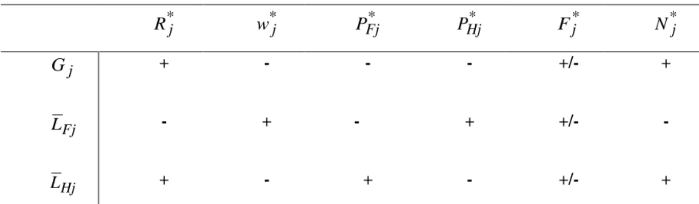
Table 2: Comparative Statics: Land-Use Regulations
* j R w*j PFj* PHj* F*j N*j j
G
+ - - - +/- + Fj L - + - + +/- - Hj L + - + - +/- +Note: A “+” ( “-”) indicates that the sign if the derivative is positive (negative). A “+/-” indicates that the sign of the derivative may be positive or negative.
Impact of an increase in the stringency of floor-space regulations (G ) j
Let’s assume a given level of household amenities and firms. First, because stringent production regulations increase production costs of office-commercial floor space, real estate developers require higher commercial rents in order to satisfy current demand for floor-space. However, office-commercial firms must be compensated with lower labor costs to offset their incentives to move. This in turn implies that households must be compensated with lower residential land rents in order to equalize utility across locations. Second, because office-commercial firms pay lower wages but higher rentals, the equilibrium number of workers/households is still higher in the location with more stringent regulations on office-commercial construction. Finally, the impact of an increase in G on the j equilibrium office-commercial land price is negative as it decreases land’s productivity.
9 These results are also consistent with previous theoretical results within the housing market which have shown
that in cases where an amenity affects positively households but it is detrimental to firms, the comparative static effects are ambiguous, with wages and rents rising or falling in almost all the cases (Blomquist 1988; Hoehn et al. 1987). For instance, in the housing-price regressions of Hoehn et al. (1987) and Blomquist et al. (1988), better public safety (lower crime) leads to lower rather than higher housing prices and in the hedonic wage regression higher particulate pollution reduces rather than increases income. Considering only the effect on wages or the effect on rents would thus suggest in the latter cases that public safety is a disamenity while pollution is an amenity. Yet, when the effects on wages and rents are both accounted for, then we observe that indeed public safety is an amenity while pollution is a disamenity.
19
Impact of an increase in the stringency of office-commercial zoning (LFj)
A lower amount of land designated for office-commercial development must be associated with higher office-commercial land prices to equalize land demand to the constrained supply. This, in turn, requires higher office-commercial floor-space rents, and therefore, a lower wage to maintain firm indifference at the unit production cost. Office-commercial firms are able to pay less for labor since households are willing to trade lower wages for lower residential land rents to equalize utility to the exogenous uniform level. As a result, the number of demanded workers in city j by each office-commercial firm is higher in the new equilibrium.
Impact of an increase in the stringency of residential zoning (LHj)
On the other hand, a lower amount of land designated for residential development must be associated with higher residential land prices which require higher wages to keep a current household indifferent across locations. This leads firms to trade higher labor costs for lower office-commercial rents in order not to move. The decrease in office-commercial rents then decreases the price of office-commercial land.
From the combined analysis of LFj and LHj, we notice that in the absence of externalities, reducing the amount of land allowed in a certain use raises the land price of that use but decreases the land price of the remaining land uses. In addition, the floor-space output associated with the restricted land use declines while its price rises and the floor-space output price associated with the unrestricted land use drops. Therefore, allowable use zoning affects land values differently across uses. On the other hand, an institutional constraint on production raises the floor-space output price associated with the restricted land use. However, and in contrast to the allowable use zoning, it affects land values equally across land uses.
5. The Empirical Model
5.1. Hedonic Analysis
The literature for quality-of-life amenities and quality-of-business amenities estimate reduced form equations of equilibrium wage and housing prices in order to explain how prices vary with amenity levels across cities. However, our main goal is to examine the determinants of intra-metropolitan variations in non-residential prices focusing on the role of local amenities. As such, we aim to estimate the reduce form (25) which includes not only quality-of-life amenities but also productive amenities and local institutional restrictions as well as a herd behavior around neighboring property prices where price expectations are formed based on neighboring values.
20
Given its multimodal structure, heterogeneity across nodes, surrounding jurisdictions and environmental amenities, Los Angeles County provides an appropriate spatial setting to illustrate the theory developed in session 3. Before describing in some detail the datasets and the variables used in our empirical exercise, the specific empirical formulation, which builds on the theoretical formulation in (25) and accounts for the spatial nature of the data available, is discussed. Our model for the hedonic regressions follows
T t i t t i i i i it G N W X Y LP 1 0 . (27)In (27) LPit represents the natural logarithm of the sale price of property i in year t, 2005
1997
t . Gi is a vector of green amenities. Ni is a vector of nearby amenities and controls. i
W is a vector of workforce characteristics. Xi is a vector of building characteristics and Yt is a dummy variable indicating the year the property was sold. The model given by (27) is our baseline model to which we compare the spatial specifications.
5.2. Spatial Analysis of Non-Residential Property Values
Our theoretical model reveals that spatial autocorrelation of a property price may result from a herd behavior around neighboring property prices where price expectations are formed based on neighboring values. This herd effect from comparable sales prices then leads to the spatial lag model where a spatially lagged dependent variable (spatially weighted neighboring prices) helps to explain the determination of property prices.
There are nevertheless two other sources of spatially correlated property prices: common omitted explanatory variable(s) and measurement error(s). The location of a property influences its selling price but nearby properties will also be affected by the same location factors. Since the inclusion of all relevant attributes is seldom fulfilled and the effects of all omitted variables are subsumed into the error term, if the omitted variables are spatially correlated, so are the regression errors. A measurement error that affects nearby properties will result in spatially correlated errors in a similar way. Both of them lead to the specification of spatial error model.
Therefore, if property prices are spatially correlated, either in their levels or in the errors, then simple OLS regression can give spurious results. Spatial econometrics explicitly accounts for the influence of space in real estate and urban models.
21 5.3. Our Empirical Strategy
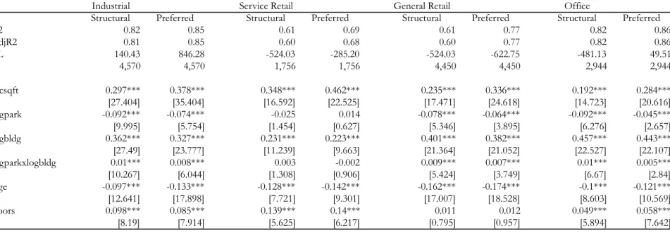
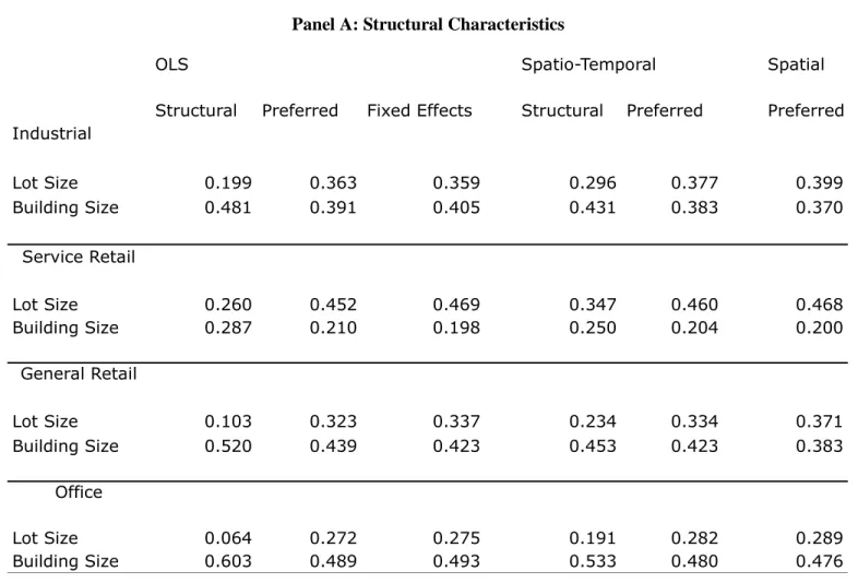
Our goal for this paper is to establish whether there are robust associations between various local amenities and the prices of non-residential properties. We aim to investigate whether there are durable associations or whether the amenity variables are simply capturing local unobservables. To this end we run specifications with a number of different sets of controls and combinations of variables and examine whether there are significant changes in sign and magnitude of the key coefficients.
The properties are classified into several broad property types including offices, industrial properties, and two types of retail. We hypothesize that office properties should be more sensitive to green, and neighborhood amenities because high-skill workers have been shown to have greater taste for these amenities. Production amenities are more mixed. The concentration of high skill workers should have a positive impact on office prices, but an unknown impact of industrial and retail prices. Other amenities such as rail access, freeway access, or airport proximity may have impacts on all property types. Differences in amenity value between the different property types are a signal that the regressions are capturing correlations between amenities and prices.
Studies focused on characteristics of the property or structure, such as an environmental label, can use a fixed effects strategy, however, fixed effects will eliminate the influence of the amenities we wish to examine. Nearby properties are likely to have similar unobservable characteristics and spatial regression controls for these. We use a spatial method that allows for both spatial autocorrelation and spatial lag. That is, the specification allows for the errors and the dependent variable to be correlated across nearby observations.
Spatial Models
Spatial methods have been used sparingly in the non-residential real estate literature, and to our knowledge they have never been used to examine the relationship between amenities and non-residential real estate prices. The specification is the same as in (27) except:
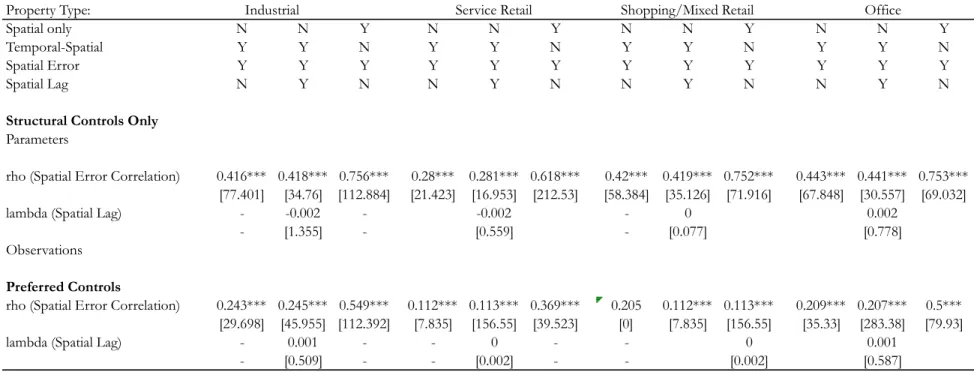
u e W LP W 1 2 (28) where measures the degree of spatial autocorrelation, W1 is a weighting matrix, LP is the vector of
property prices, is a scalar measuring the degree of spatial error correlation, W2 is another (possibly distinct) weighting matrix, and e and u are i.i.d disturbances.10
10 In order to test the robustness of our results to alternative specifications of our k-nearest neighbor matrix, we
computed different matrices on the basis of the 8th, 10th, 15th and 30th closest neighbor criteria. While our coefficient
estimates aren't much different between the runs, the spatial dependence declines with the increasing number of nearest neighbors taken into account. Our final runs are at 10 but with a mile cutoff, which only affects a few properties but avoided some clusters where properties are very far apart.
22
Using the weights matrix, the lag operator W1LP captures the spatially weighted average of the variable of interest in a given location. This is analogous to our theoretical term [Pj,t] in equation (25). Thus, the spatial variable captures the impact of the neighboring unit valuations on the transaction price of a property. One of the innovative features of our spatial model is the construction of an integrated spatio-temporal weights matrix, following the methodology of Dube and Legros (2013, 2015). This spatio-temporal weights matrix allows us to incorporate the temporal dimension of the data generating process of spatial data pooled over time.
Spatio-Temporal Weights Matrices (W1 and W2)
Typical spatial econometric methods ignore the influence of time on spatial dependence. However, with data over eight years the assumption that there is no temporal dimension to spatial autocorrelation is unlikely to be true. For instance, it is unlikely to be either spatial or error correlation with a property that is sold several years in the future.
Following Dube and Legros (2013, 2015), we can obtain the spatio-temporal weights matrix (W ) by separating its construction into a spatial (S) and temporal ( T ) weighting matrices. While S uses an inverse Euclidean distance function to determine the impact of neighboring transactions based on geographical proximity and a critical cut-off miles distance, T takes temporal dependence through an inverse function of the time elapsed between realization of two transactions with cut-offs memory effects for both future and past transactions. In particular, each element ti,jof the temporal matrix T is given by:
t
i, j=
(v
i- v
j)
-gif v
i- v
j£ v
p;"i ¹ j and v
i> v
jv
i- v
j-gif v
i- v
j£ v
f;"i ¹ j and v
i< v
j1 if v
i= v
j0 otherwise
ì
í
ï
ïï
î
ï
ï
ï
(29)where vi and v are the time (quarterly values in our case) when properties i and j j are sold respectively,
v
p is a cut-off value for past transactions (sales),v
f is a cut-off value for future transactions, and is a parameter that determines how fast observations fade in importance as the distance in time increases (time fade parameter). We test different values for these parameters with our data. Since the transactions are ordered chronologically, the lower triangular matrix of T contains actual and past transactions, while the upper triangular matrix contains actual and future transactions. Finally, to incorporate the simultaneity of both spatial and temporal relations, we multiply, term by term, the two23
developed relations matrices Sand T , resulting in our spatio-temporal matrix W ST, with the Hadamard matricial product. We also examined a variety of spatial and temporal weight matrices for both the error and spatial lag.
If is significant, then the non-spatial estimate will generally be biased. Therefore, it is important to test for spatial autocorrelation. Not accounting for spatial error correlation does not bias coefficients, but does result in inefficient estimation. We also examined results across property types and with different sets of local controls in the spatial framework. If coefficients on amenities in the spatial regressions are significant in the expected direction and differ across property types in expected ways, then that is evidence that the amenity coefficients are capturing a real association as opposed to capturing local unobservables.
5.4. Data and Variables
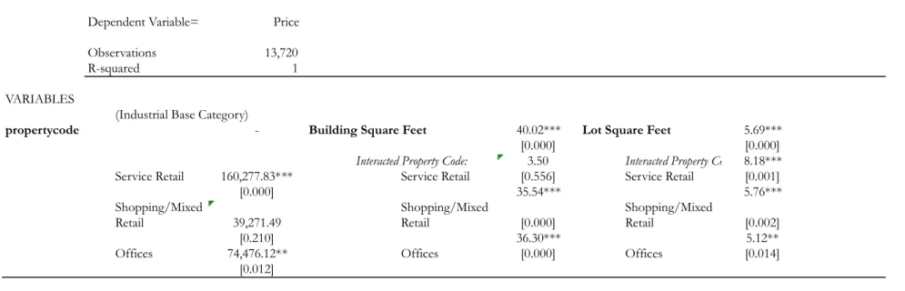
Parcel-level data on non-residential property sales from 1996 through 2005 over a significant portion of Los Angeles County was obtained through Costar Group, a national commercial real estate information provider (www.costar.com). After removing several types of parcels not suitable for the analysis and data with missing variables we were left with 13,370 observations.11 The database contains
the sales price of each property and a vector of structural characteristics (such as building coverage, permeable area, building square footage, and parking lot spaces, and property code).
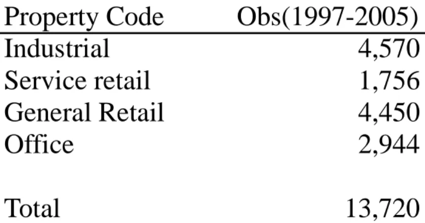
The initial database assigned each observation as one of three general land use types: industrial, office or retail. We divide properties into 4 classes of non-residential use: (1) industrial, which includes manufacturing, warehouse, and other industrial uses; (2) Office properties; (3) service retail, which includes banks, restaurants, various services businesses such as doctor’s offices, and auto related services; and, (4) mixed and shopping retail, the last includes many small shopping centers with shopping as well as some service retail storefronts (see Table 3 in the Appendix).12
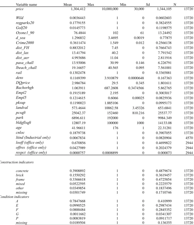
Our variables come from many different data sets. Tables 4 and 5 in the Appendix detail the variables and show the summary statistics, respectively.
We look at several types of green amenities including air quality, proximity to parks, wilderness, and shore, weather, and shore proximity. For air quality, we found that the average level of pollutants is very similar across all areas of the county. The main difference is in the right tails of the distribution
11 We removed several types of parcels which were not suitable for the analysis, namely parking, public facilities,
residential, heavy industrial, industrial park, pleasure retail, retail-residential, retail-office, hi-rise-office. We also removed categories where there were few observations and where it was not clear how to group them with other categories. Also, we dropped observations from 1996 because there were few observations. We also dropped any repeat sales which were just a few observations to begin with.
12 Light industrial and industrial were combined into industrial and office-residential, office-industrial and lo-rise