Image reconstruction algorithm implementation for the easyPET: a didactic and pre-clinical PET system

FACULDADE DE CIÊNCIAS

DEPARTAMENTO DE FÍSICA

Image Reconstruction Algorithm Implementation for the

easyPET: a didactic and pre-clinical PET system

Pedro Miguel Martins de Sousa e Sá

Mestrado Integrado em Engenharia Biomédica e Biofísica

Perfil em Radiações em Diagnóstico e Terapia

Dissertação orientada por:

Dr. Nuno Matela

i

ACKNOWLEDGEMENTS

Firstly, I would like to acknowledge the people that are part of the easyPET project and with whom I have worked with. To Prof. Dr. João Veloso, Prof. Dr. Pedro Almeida, and Prof. Dr. Nuno Matela for having allowed me to participate in such innovative project and develop the work presented in this thesis. To Pedro Correia, the right person to work with, given his friendliness, and willingness and objectivity when discussing matters. To Joana Menoita who has produced part of the results presented here. Finally, to all the participants in this project, whom have brought the easyPET so far, might it go as far as intended.

To my supervisor, Prof. Dr. Nuno Matela, with whom I deeply appreciate having worked with, given his friendliness and availability, with the occasional football discussions and moderate club rivalry. Even more, I would like to acknowledge the interest and knowledge on Biomedical Engineering he has conveyed to me during my academical journey, culminating with this thesis. I truly am thankful to him. To all the persons I have met at IBEB until this moment, all the Professors, researchers, and students. People have come and go, but it remains a special place to work in, and I could not be more thankful. On a special notice, I would like to acknowledge Beatriz Lampreia, for being a friendly face at all times. For the time I have spent at IBEB, most was in the company of Nuno Santos, with whom I am very happy to have become friends with. Currently, me and Leon Vink are still resilient in leaving.

To the people I have met throughout my academic path, in one way or another, you have contributed to my success. To Francisco Geraldes, Joaquim Costa, and Rui Marcelino, it has been a good ride. Finally, and after all, it was up to my family to put me in this world. The effort and dedication I have seen and know in my parents and grandparents have no bounds. Life does not always come easy, but it is no excuse to stop and not work for the best. To my brother, well, being the youngest is no longer terrible. I sure am glad you did not push me off the nest when you had the chance.

ii

RESUMO

Tomografia por Emissão de Positrões (PET) é uma técnica de imagiologia funcional, utilizada para observar processos biológicos. O conceito de tomografia por emissão foi introduzido durante a década de 1950, sendo que foi apenas com o desenvolvimento de radiofármacos na década de 1970, que esta técnica começou a ser utilizada em medicina. Nos últimos 20 anos, o avanço tecnológico tornou os sistemas PET numa ferramenta altamente qualificada para imagiologia funcional. Neste período, o aparecimento de sistemas PET-CT veio colmatar as deficiências produzidas pela PET ao nível de imagem estrutural, com a combinação desta técnica funcional com a de Tomografia Computadorizada (CT). A evolução da tecnologia PET foi também acompanhada pela evolução da tecnologia para produção de radiofármacos, incluindo os radionuclídeos, bem como do conhecimento médico relativo aos processos biológicos humanos. Aliando esta tecnologia e conhecimento, tornou-se possível traçar moléculas com funções metabólicas nos diversos sistemas do corpo humano e, assim, produzir uma variedade de imagens funcionais.

Dado o tipo de imagem produzida pela técnica PET, é bastante comum associar-lhe o diagnóstico de doenças cancerígenas, cuja principal característica é a desregulação metabólica celular no organismo. Tendo em vista o aumento esperado da incidência de cancro em Portugal e na Europa, tendo já sido atingida uma incidência nacional, em 2010, de 444,50 pessoas em cada 100.000 (números avançados pela DGS, 2015), a utilização de técnicas que permitam o diagnóstico precoce destas doenças é de elevada importância. Posto isto, e apesar do constante crescimento do gasto público em cuidados médicos relativos ao diagnóstico e tratamento de cancro, estão a ser postos cada vez mais esforços e fundos para que o processo de Investigação e Desenvolvimento (I&D) relacionado com esta doença seja célere. São constantemente desenvolvidas novas e melhores técnicas de imagiologia, que permitem diagnósticos mais precoces e precisos, enquanto ajudam na aplicação de planos de tratamento mais eficazes que, consequentemente, levam a um gasto público mais eficiente.

Os sistemas PET inserem-se neste contexto e, uma vez permitindo imagem altamente sensível a processos funcionais, facilmente se generalizaram no meio médico e académico. Os sistemas direcionados a aplicações relacionadas com a medicina humana têm como função observar processos biológicos, com a finalidade de um diagnóstico médico ou estudo. Sistemas pré-clínicos, direcionados a estudos com animais pequenos, têm o propósito de auxiliar a investigação relacionada com os estudos preliminares de doenças que afetem o ser humano. Finalmente, e sendo o grupo com menor oferta comercial, os sistemas PET didáticos possibilitam uma melhor formação de pessoal responsável pelo futuro uso e I&D relacionados com esta tecnologia. No entanto, a tecnologia utilizada nestes três tipos de sistemas encarece consideravelmente o seu valor comercial sendo que, contrariamente ao que seria de esperar, os preços dos sistemas pré-clínicos não se diferenciam consideravelmente dos sistemas para humanos. O encarecimento destes sistemas deve-se ao facto de que toda a tecnologia a eles associada tem características mais dispendiosas de produzir. No caso dos sistemas didáticos, simplesmente não existe o incentivo necessário à sua produção e compra.

É neste contexto que surge o easyPET. O design inovador, constituído por apenas duas colunas de detetores opostos, e tirando partido de uma atuação sobre dois eixos de rotação, faz deste sistema ideal para entrar no mercado em duas vertentes. A primeira, constituída apenas por um detetor em cada coluna, está destinada a ter um papel didático. A segunda, tirando partido de colunas com múltiplos detetores, foi desenhada para entrar no mercado de sistemas pré-clínicos. Em ambos os casos, a principal característica do easyPET, e a que o destaca dos restantes sistemas, é o seu reduzido número de detetores, que resulta num reduzido custo de produção. Através da implementação de um número reduzido de detetores e, consequentemente, reduzida eletrónica, é possível obter um custo final da máquina inferior.

iii

No entanto, é sempre necessário garantir que os dados obtidos em tal sistema correspondam a imagens com as características necessárias, sendo que o processo de reconstrução de imagem é bastante importante.

O trabalho apresentado nesta tese tem como objetivo a implementação de um método de reconstrução de imagem a duas dimensões, dedicado ao sistema easyPET. Para tal, foi considerado um algoritmo estatístico iterativo que se baseia na Maximização da Estimativa da Máxima Verosimilhança (ML-EM), introduzido por Shepp e Vardi em 1982. Desde então, tem sido largamente explorado e, inclusive, dando aso a outras versões bastante comuns em reconstrução de imagem PET, como é caso da Maximização da Espectativa usando Subgrupos Ordenados (OS-EM).

A implementação do algoritmo escolhido foi feita no software Matlab. Para computar a unidade básica do algoritmo, a Linha de Resposta (LOR), foi implementado o método ray-driven. Por forma a otimizar a construção da matriz de sistema utilizada neste algoritmo, foram implementadas simetrias de geometria. Esta otimização baseou-se na consideração de que a geometria do sistema easyPET pode ser dividida em quadrantes, sendo que um único quadrante consegue descrever os restantes três. Além disso, foram também implementadas otimizações ao nível estrutural do código escrito em Matlab. Estas foram feitas tendo em conta o aumento na facilidade de acesso à memória através da utilização variáveis para rápido indexamento. Foram também implementados dois métodos de regularização de dados: filtragem gaussiana entre iterações e um root prior baseado na mediana. Por forma a comparar, mais tarde, os resultados obtidos através do algoritmo implementado, foi também implementado o método de reconstrução de Retroprojeção Filtrada (FBP). Por último, foi implementada uma interface para o utilizador, utilizando a aplicação GUIDE do Matlab. Esta interface tem como objetivo servir de ponte entre o sistema didático easyPET e o utilizador, para que a experiência de utilização seja otimizada. Por forma a delinear o teste ao sistema easyPET e ao algoritmo ML-EM implementado, foram seguidas as normas NEMA. Este é um conjunto de normas que tem como objetivo padronizar a análise realizada a sistemas de imagem médica. Para tal, foram adquiridos e simulados ficheiros de dados com uma fonte pontual a 5, 10, 15 e 25 mm do centro do campo de visão do sistema (FOV) e utilizando um par de detetores com 2x2x30 mm3_{. Para realizar a análise de resultados, os dados foram reconstruídos}

utilizando a FBP implementada, e foi medida a FWHM e FWTM da fonte reconstruída. O mesmo procedimento foi aplicado, mas reconstruindo os dados através do algoritmo ML-EM, utilizando o filtro gaussiano, o MRP, e não utilizando qualquer método de regularização de dados (nativo). Por forma a comparar os métodos de regularização de dados, foi também realizada uma medição do rácio sinal-ruído (SNR). Os resultados foram obtidos para imagens reconstruídas com um pixel de, aproximadamente, 0.25x0.25 mm2_{, correspondendo a imagens de 230x230 pixeis.}

Os primeiros resultados foram obtidos a fim de determinar qual a iteração em que se começaria a observar a estabilização das imagens reconstruídas. Para algoritmo ML-EM implementado e o tipo de dados utilizados, foi observado que a partir da 10a _{iteração o algoritmo ML-EM converge. Através das}

medidas para a FWHM e FWTM observou-se, também, que os dados obtidos experimentalmente se diferenciam dos resultados obtidos sobre os dados simulados. Isto levou a que, fora dos objetivos deste trabalho, fossem realizados mais testes utilizando dados experimentais e, que daqui em diante, apenas fossem utilizados dados obtidos através de simulação Monte Carlo, por razões de conveniência na precisão da colocação da fonte pontual. De seguida, comparam-se os dados obtidos através da FBP e o algoritmo ML-EM nativo. Para o primeiro caso foram medidas FWHM de 1.5x1.5 mm2_{, enquanto que}

para o segundo foram atingidos valores de 1.2x1.2 mm2_{. Para os métodos de regularização de dados}

foram medidos valores de resolução semelhantes ou inferiores, sendo que estes resultaram num aumento da qualidade da reconstrução da fonte, observado através do aumento no valor de SNR medido.

iv

O trabalho apresentado nesta tese revela, não só a validação do algoritmo de reconstrução proposto, mas também o bom funcionamento e potencialidades do sistema easyPET. Pelos resultados obtidos através das normas NEMA, é possível observar que este sistema vai ao encontro do estado de arte. Mais ainda, através de um método de reconstrução dedicado ao easyPET é possível otimizar os resultados obtidos. Com o avançar do projeto no qual este trabalho esteve inserido, é de esperar que o modelo a três dimensões pré-clínico easyPET irá produzir melhores resultados. De frisar que o sistema easyPET didático se encontra na sua fase final e que os resultados obtidos são bastante satisfatórios tendo em conta a finalidade deste sistema.

Palavras Chave: Tomografia por Emissão de Positrões (PET)

Reconstrução de Imagem em PET

Maximização da Espectativa da Máxima Verosimilhança (ML-EM) Resolução Espacial

v

ABSTRACT

The easyPET scanner has an innovative design, comprising only two array columns facing each other, and with an actuation defined by two rotation axes. Using this design, two approaches have been taken. The first concerns to a didactic PET scanner, where the arrays of detectors are comprised of only one detector each, and it is meant to be a simple 2-dimensional PET scanner for educational purposes. The second corresponds to a pre-clinical scanner, with the arrays having multiple detectors, meant to acquire 3-dimensional data. Given the geometry of the system, there is no concern with the effects of not measuring the Depth-of-Interaction (DOI), and a resolution of 1-1.5 mm is expected with the didactic system, improving with the pre-clinical. The work presented in this thesis deals with 2D image reconstruction for the easyPET scanners.

The unconventional nature of the acquisition geometry, the large amount of data to be processed, the complexity of implementing a PET image reconstruction algorithm, and the implementation of data regularization methods, gaussian filtering and Median Root Prior (MRP), were addressed in this thesis. For this, the Matlab software was used to implement the ML-EM algorithm. Alongside, several optimizations were also implemented in order to convey a better computational performance to the algorithm. These optimizations refer to using geometry symmetries and fast indexing approaches. Moreover, a user interface was created so as to enhance the user experience for the didactic easyPET system.

The validation of the implemented algorithm was performed using Monte Carlo simulated, and acquired data. The first results obtained indicate that the optimizations implemented on the algorithm have successfully reduced the image reconstruction time. On top of that, the system was tested according to the NEMA rules. A comparison was then made between reconstructed images produced by using Filtered Back Projection (FBP), the native ML-EM implementation, the ML-EM algorithm using inter-iteration gaussian filtering, and the ML-EM algorithm implemented with the MRP. This comparison was made through the calculation of FWHM, FWTM, and SNR, at different spatial positions. The results obtained reveal an approximate 1.5x 1.5 mm2 _{FWHMsource resolution in the FOV, when recurring to}

FBP, and 1.2x 1.2 mm2 _{for the native ML-EM algorithm. The implemented data regularization methods}

produced similar or improved spatial resolution results, whilst improving the source’s SNR values. The results obtained show the potential in the easyPET systems. Since the didactic scanner is already on its final stage, the next step will be to further test the pre-clinical system.

Keywords Positron Emission Tomography (PET)

PET Image Reconstruction

Maximum Likelihood Expectation Maximization (ML-EM) Spatial Resolution

vi

INDEX

Acknowledgements... i Resumo... ii Abstract... v List of Figures... ix List of Tables... xi

List of Abbreviations... xii

1 Introduction ... 1

1.1 PET Technique Evolution and Role in Medicine ... 1

2 Background ... 2

2.1 Molecules and Tracers ... 2

2.2 Basic Physics ... 2

2.2.1 β+ decay ... 2

2.2.2 Positron Annihilation ... 3

2.3 Event Detection, Coincidence, and Detector Bins ... 4

2.3.1 Scintillator ... 4

2.3.2 Photodetector ... 4

2.3.3 PET Detector and Coincidence Detection ... 5

3 PET Data Output and Representation... 6

3.1 System’s Output – PET Data ... 6

3.1.1 List Mode and its Post-Processing ... 6

3.2 LOR ... 6

3.2.1 LOR Computing and System Matrix ... 7

3.3 Sinogram ... 7

4 Image Reconstruction ... 8

4.1 Image Reconstruction Algorithm ... 8

4.2 Iterative Algorithms and Expectation Maximization (EM) ... 8

4.2.1 Maximum Likelihood Expectation Maximization (ML-EM)... 9

4.2.2 OS-EM and GPU Implementations ... 10

4.3 Filtered Back Projection (FBP) ... 10

5 Data Correction and Regularization Methods ... 12

5.1 Data Corrections ... 12

5.1.1 Attenuation Correction ... 12

5.1.2 Time of Flight (ToF) ... 12

5.1.3 False Coincidences – Scatter and Random Coincidences ... 13

vii

5.1.5 Depth of Interaction (DOI) ... 14

5.2 Data Regularization Methods ... 15

5.2.1 Inter-Iteration Gaussian Filtering ... 15

5.2.2 Median Root Prior (MRP) ... 15

5.3 Image Resolution and Quality Assessment ... 16

5.3.1 Image and Spatial Resolution ... 16

6 PET Systems ... 17

6.1 Didactic, Pre-Clinical, and Human Scanners ... 17

6.2 Scanners Geometries and Dimensional Acquisition ... 17

6.3 State of the Art ... 18

6.3.1 DigiPET – MEDISIP/INFINITY ... 18

6.3.2 β-cube – Molecubes/IBiTech/MEDISIP/INFINITY ... 19

6.3.3 NanoScan PET/MRI – MEDISO... 19

6.3.4 Albira PET/SPECT/CT – MILabs ... 20

7 easyPET System ... 21

7.1 Project and Work Group ... 21

7.2 Concept Geometry ... 21

7.3 Hardware and Actuation ... 22

7.4 3-Dimensional Acquisition Mode ... 22

8 Motivation ... 23

9 Materials and Methods ... 24

9.1 Matlab software ... 24

9.2 easyPET system acquisition ... 24

9.3 easyPET Data ... 25

9.3.1 List Mode ... 25

9.3.2 Processing the List Mode ... 25

9.4 LOR and System Matrix ... 26

9.4.1 LOR ... 26

9.4.2 System Matrix ... 27

9.5 ML-EM and Code Optimizations ... 28

9.5.1 Building the Algorithm ... 29

9.5.2 Implementing Optimizations ... 31

9.6 Image Enhancement Implementations ... 32

9.6.1 Gaussian Filtering ... 32

9.6.2 Median Root Prior (MRP) ... 32

9.7 Filtered Back Projection Implementation ... 33

viii

9.8.1 NEMA Rules ... 33

9.8.2 Data for Reconstruction ... 34

9.8.3 Algorithm Validation ... 34

9.8.4 Image quality assessment ... 34

10 Results ... 36

10.1 GUI ... 36

10.1.1 User Interaction ... 36

10.1.2 Advanced GUI ... 38

10.2 Image Analysis Results ... 38

10.2.1 ML-EM convergence ... 39

10.2.2 Acquired versus Simulated Data ... 39

10.2.3 NEMA Rules Comparison versus ML-EM Algorithm... 41

10.2.4 Data Regularization Methods Comparison ... 42

10.2.5 Source Resolution ... 42 10.2.6 Source SNR ... 43 10.3 Final Discussion ... 44 11 Conclusion ... 47 12 Future Work ... 48 13 References ... 49

ix

List of Figures

Figure 2.1: Annihilation process known in elementary physics. A positron (e+) is emitted from the atomic nucleus together with a neutrino (v). The positron is ejected randomly and travels through

matter until colliding with an electron (e-), hence producing an annihilation [4]. ... 3

Figure 2.2: Schematic of a photomultiplier tube coupled to a scintillator [5]. ... 4

Figure 3.1: Representation of a LOR in the 2D space, given an annihilation that activates the detectors in red. s is the distance to the center of the FOV. 𝜙 is the angle of rotation defined by s. Adapted from [9]. ... 7

Figure 3.2: A centered point source and an off-centered point source in the scanner (a) describe, respectively, a straight line and a sinusoidal line in the sinogram (b). Adapted from [10]. ... 7

Figure 4.1: Schematic overview of an iterative Expectation Maximization (EM) reconstruction algorithm. ... 9

Figure 5.1: Representation of the effect caused by photon attenuation, with and without attenuation correction [25]. ... 12

Figure 5.2: Compared to conventional PET, the estimated ToF difference (∆𝑡) between the arrival times of photons on both detectors in TOF-PET allows localization (with a certain probability) of the point of annihilation on the LOR. In TOF-PET, the distance to the origin of scanner (∆x) is proportional to the TOF difference via the relation ∆𝑥 = 𝑐∆𝑡2, where 𝑐 is the speed of light, 𝑡1 the arrival time on the first detector, and 𝑡2 is the arrival time on the second detector [26]. ... 13

Figure 5.3: Type of coincidences in PET [27]. ... 13

Figure 5.4: A) For a point source near the center of the FOV, photons enter crystals in the detector array through their very small front faces and the difference between the LORs and the true photon flight paths is small, i.e. results in “good” radial resolution. B) For off-axis sources, photons can enter the crystals through their front faces and anywhere along their sides, so radial resolution is “poor”. Note that tangential resolution is not dependent on the DOI effect and is essentially constant across the FOV [31]. ... 14

Figure 5.5: Noise presence in sources combined with poisson noise to demonstrate the noisy nature of PET imaging. The images shown correspond to a) 10 counts per pixel; b) 100 counts per pixel; c) 1000 counts per pixel; d) 10000 counts per pixel. ... 15

Figure 6.1: Representation of a 3D ring assembly of PET detectors [36]. ... 18

Figure 6.2: Schematics of the DigiPET system prototype [37]. ... 19

Figure 6.3: Schematic axial cut of the 𝛽-cube [38]. ... 19

Figure 6.4: nanoScan small-animal PET/MR scanner schematics. Labeled components are: (1) PET ring; (2) magnet; (3) radiofrequency coil. The increased size concerns to the difficulty in combining these two techniques [39]. ... 20

Figure 6.5: Schematic view of the entire Albira PET/SPECT/CT system [40]... 20

Figure 7.1: Schematic for the easyPET geometry, retrieved from the patent file. (1) corresponds to the bottom/𝛼 angle axis of rotation; (2) corresponds to the top/𝜃 angle axis of rotation; (3) and (4) correspond to the two detector arrays. Note that the top/𝜃 angle axis of rotation is fixed in (3), more specifically the detector’s face. Left: schematic for a bottom/𝛼 angle revolution. Right: schematic for the fan-like movement, defined by the top/𝜃 angle, performed at each bottom/𝛼 angle step. Adapted from the easyPET system’s patent. ... 21

Figure 7.2: Image used for commercial purposes by Caen, portraying the U-shape PCB with two detectors, one at each U-tip [37]. ... 22

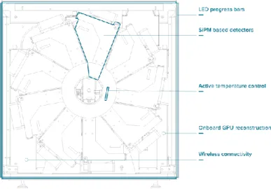
Figure 7.3: Design for the pre-clinical easyPET scanner [44]. ... 23

Figure 9.1:View of a LOR projected into the transaxial plane, where the LOR is described by the coordinate pair (𝑠, 𝜙). Adapted from [48]. ... 26

x

Figure 9.2: Representation of the ray-driven method. For simplicity, each detector's face's middle point is considered in contact with the FOV. ... 27 Figure 9.3: Scripted code to exemplify the implementation of the Forward Projection operation. ... 29 Figure 9.4: Scripted code to exemplify the implementation of the Back Projection operation. ... 30 Figure 9.5: Scripted code to exemplify the implementation of the Image normalization operation, inside the Back Projection operation. ... 30 Figure 9.6: Scripted code to exemplify the implementation of the image reconstruction ML-EM algorithm. Note that an alteration is made inside the BackProjection Operation to accommodate the use of the operator that results from the Forward Projection, and, also, the image iteration. ... 31 Figure 9.7: Schematic on how the ellipse ROI and the profile lines are defined. ... 35 Figure 10.1: Set up of the GUI with data inputted as example. Images acquired with: (1) ML-EM algorithm; (2) Simple back projection; (3) sinogram representation; (4) Filtered Back Projection. ... 37 Figure 10.2: Current user interface developed. This interface allows control over the system

acquisition, overview over the acquisition parameters, image statistics, and image back projection. This image was produced at RI.TE for the 1st _{Workshop on the Development of easyPET}

Technologies. ... 38 Figure 10.3: Graph illustrating the results obtained for FWHM and FWTM of the ML-EM algorithm, showing the algorithm’s convergence around the 10th _{iteration. ... 39}

Figure 10.4: Graph illustrating the results obtained at FWHM. with the ML-EM algorithm and the FBP, using acquired and simulated data, at: 0.56, 0.75, 6, 8.1, 10.3, 12.54, and 15 mm from the center of the FOV. ... 40 Figure 10.5: Graph illustrating the results obtained for a point source at: 5, 10, 15, and 25 mm from the center of the FOV. The FWHM and FWTM were measured in the x direction (dashed lines) and y direction (full lines), for the ML-EM algorithm (circle points) and FBP (square points). ... 41 Figure 10.6: Example of how the point sources were reconstructed using: (1) FBP; (2) native ML-EM algorithm; (3) ML-EM algorithm with inter-iteration gaussian filtering; (4) ML-EM algorithm with MRP 𝛽 = 0.33. Note that very little difference can be seen between (3) and (4), mainly due to the size of the source. (1) is clearly less round than the remainder and it is possible to see some LORs

projected. (2) source appears less smooth. ... 42 Figure 10.7: Graph illustrating the measured FWTM resolution values in x and y directions for the native ML-EM algorithm, ML-EM with inter-iterations gaussian filtering, and ML-EM algorithm with MRP and 𝛽 = 0.66. ... 43 Figure 10.8: Graph illustrating the source SNR measured at different distances from the center of the FOV using the native ML-EM algorithm, the ML-EM algorithm using inter-iteration gaussian

filtering, FBP, and ML-EM algorithm using MRP with 𝛽 = 0.33; 0.66; 1. ... 44 Figure 10.9: Graph showing the x-y directions resolution ratio for the measured FWTM and for all tested methods. ... 46

xi

List of Tables

Table 2.1: Common radionuclides used in PET, their half-lives, correspondent rediopharmaceutic, and intended object of study. ... 2 Table 2.2: Designations of common crystals used in PET detector's scintillators, and their main

attributes [5]. ... 4 Table 6.1: Summary of the systems presented above. *Algorithm used for spatial resolution

measurement following NEMA rules. **Native algorithm developed for the system. ... 20 Table 10.1: Number of coincidences detected for each simulated and acquired data file, at the

specified distance from the center of the FOV. ... 41 Table 10.2: Summary of the systems presented in Chapter 6 and, in addition, the results obtained with the easyPET system. *Algorithm used for spatial resolution measurement following NEMA rules. **Native algorithm developed for the system. ... 46

xii

List of Abbreviations

2D Two dimensional

3D Three dimensional

AOR Area of Response

BSO Bismuth Silicone Oxide

CPU Central Processing Unit

CT Computed Tomography

DOI Depth of Interaction

EM Expectation Maximization

FBP Filtered Back Projection

FDG Fludeoxyglucose

FOV Field of View

FWHM Full Width at Half Maximum

FWTM Full Width at Tenth Maximum

GSO Gadolinium Oxyorthosilicate

GPU Graphics Processing Unit

GUI Graphical User Interface

GUIDE Graphical User Interface Development Environment

keV Kilo Electronvolt

LOR Line of Response

LYSO Lutetium-yttrium Oxyorthosilicate

ML Maximum Likelihood

ML-EM Maximum Likelihood Expectation Maximization

MR Magnetic Resonance

MRP Median Root Prior

OS-EM Ordered Subset Expectation Maximization

PET Positron Emission Tomography

RAM Random Access Memory

ROI Region of Interest

SNR Signal-to-noise Ratio

SPECT Single-photon Emission Computed Tomography

TOF Time of Flight

1

1 Introduction

1.1 PET Technique Evolution and Role in Medicine

Positron Emission Tomography (PET) is a nuclear functional imaging technique, used to observe biological processes. The concept of emission tomography was first introduced in the 1950s. Soon after, the first PET scanner appeared. Yet, it was only in the 1970s, with the development of radiopharmaceuticals, that PET imaging technique saw its first breakthrough into medicine. The new millennium saw its acceptance in the medical community widened with the introduction of PET-CT imaging systems, combining both functional and structural imaging techniques.

In medicine, PET technique helps practitioners study and diagnose diseases that carry specific biomarkers, or have localized high concentrations of specific biomolecules. Most commonly, PET technique is associated with cancer diagnosis, as the abnormal cellular growth relates to erratic metabolic levels.

In 2016, and only in the USA, an estimated 1 685 200 new cases of cancer were diagnosed, while 595 690 have died. This represents an incidence of a staggering 454.8 per 100 000 persons, and a mortality of 171.2 per 100 000 [1]. Although cancer incidence is increasing, frequently associated with constant and increasing exposure to risk factors, the overall death rate for this disease is decreasing. With an ever-rising medical care expenditure on cancer diagnosis and treatment, funds and efforts are being put to cancer related research and development (R&D). New and enhanced imaging techniques are allowing more precise and earlier diagnosis, while helping form more effective treatment plans, leading to a more efficient funds expenditure.

Research on PET appears in this context. Being a highly sensitive functional imaging technique, it has become widely spread, and current PET systems range from clinical to educational applications. Systems for human applications have a purpose in diagnosing and studying biological processes. Devices for small animal’s studies are meant to aid researchers in better study diseases which relate to the human being. Finally, and being the scarcer group, didactic PET systems are helping better train people who will perform PET related work.

However, there are two main drawbacks with this technique. The first being the infrastructure needed to provide radionuclides to perform a PET scan. The second, and the one that relates the most with medical care and overall R&D, is total expenditure. Disregarding all the funds needed to start a R&D project, imaging systems, in this case PET, build up to be one of the most expensive equipment in any medical care or research facility. One would guess that small animals and didactic devices are cheaper whilst comparing to human systems. Yet, small animal’s devices use more expensive technology that allows smaller image resolution. As for didactic systems, even though they are cheaper by only allowing reduced image resolution and quality, academic institutions are not able to cope with the prices. The following written work relates to PET image reconstruction. The project in which it was developed aims to tackle the need for two different devices: a didactic and a small animal’s system, both being commercially competitive, specs wise, and as affordable as possible.

2

2 Background

In this chapter, an introduction will be made on all relevant topics regarding PET technique. Naturally, some topics will be kept as simple as possible, as it is out of this work’s scope to thoroughly explain all topics.

2.1 Molecules and Tracers

In order to study a disease using the PET technique, one has to arrange a way to track down the metabolic processes behind it. For this, two things are required: a molecule that acts as a reactant in the metabolic process to observe, and a radionuclide that can be used as a tracer for the molecule used. With these, it is possible to create a radiopharmaceutical that, ultimately, will be observed in a PET scan.

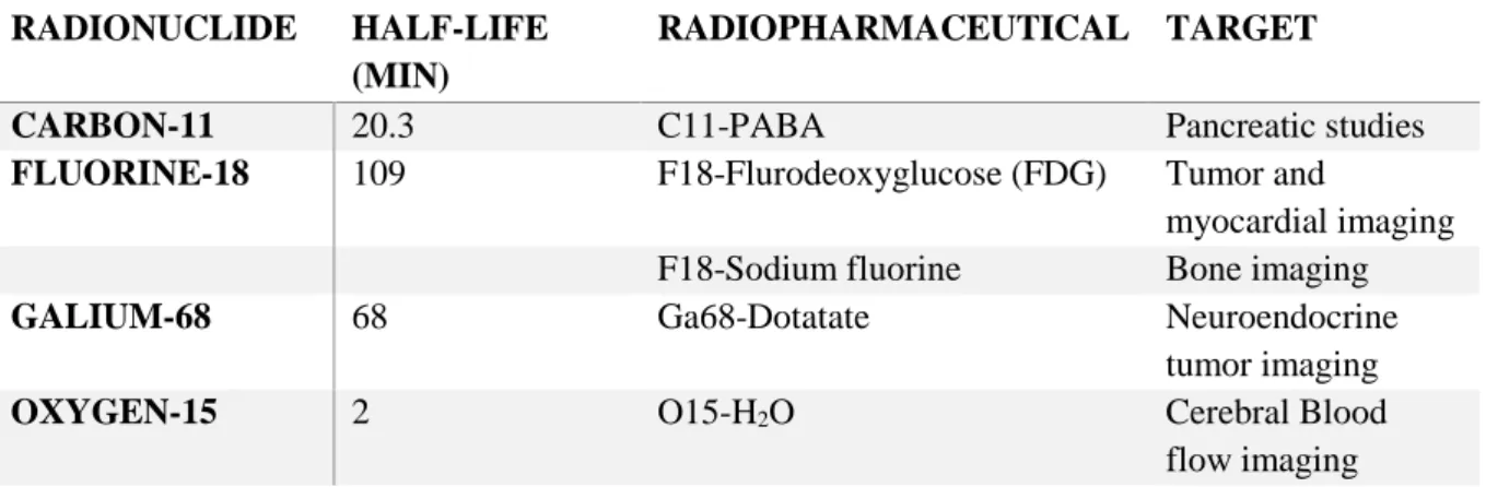
Metabolic processes occur all throughout the human body. However, when comparing with healthy subjects, diseases create changes in metabolic patterns. Depending on the focused metabolic process to be observed, reactant molecules must be chosen accordingly. Even though PET is often associated with cancer disease, where the abnormal cellular growth is known to lead to the increase region intake of glucose, radiopharmaceuticals are produced to best fit the object disease. As can be seen in Table 2.1, diseases range from stroke to lung perfusion, bone cancer, and organ failure.

What transmits the location of such molecules are radioactive tracers which, when combined with biological reactants, creates a radiopharmaceutical. These tracers are chosen depending on their half-life, which will be discussed next, commercial availability, and affinity to the chosen molecule. Some of the most common radiopharmaceuticals and their purposes can be seen in Table 2.1.

Table 2.1: Common radionuclides used in PET, their half-lives, correspondent rediopharmaceutic, and intended object of

study.

RADIONUCLIDE HALF-LIFE (MIN)

RADIOPHARMACEUTICAL TARGET

CARBON-11 20.3 C11-PABA Pancreatic studies

FLUORINE-18 109 F18-Flurodeoxyglucose (FDG) Tumor and

myocardial imaging F18-Sodium fluorine Bone imaging

GALIUM-68 68 Ga68-Dotatate Neuroendocrine tumor imaging

OXYGEN-15 2 O15-H2O Cerebral Blood

flow imaging

2.2 Basic Physics

2.2.1

𝛃+ decay

As the name states, this imaging technique relies on positron emission. Used positron emitting radionuclides are produced in a ciclotron and, usually, the isotopes are chosen to have short half-lives, when comparing to other well-known radioactive isotopes (Uranium, Plutonium, etc). The shorter half-lives are compatible with the biological processes aimed for observation. Stable nuclei like oxygen-16, carbon-14, etc., found in metabolic reactants, such as water, glucose, and ammonia, are replaced by the correspondent isotopes (e.g. oxygen-15, carbon-11, etc.). Yet, radionuclides can also be chosen to trace synthetic drugs delivered to our body. All around, these labelled compounds are called radiotracers and

3

are used to find the source or distribution of a given disease in PET exams. Note that isotopes are also chosen based on their half-lives. For optimal results, the time any given compound takes to reach its intended target should match, within reason, with the isotope’s half-life [2].

Positron emission (𝛽+ decay) is a subtype of radioactive decay. It is represented by a proton turning into a neutron by emitting a positron (Equation 2.1).

𝑝 → 𝑒++ 𝑛 + 𝑣𝑒 ( 2.1 )

Positron emission takes place when a nucleus is unstable due to an imbalance between protons and neutrons. In 𝛽+ decay, this state is balanced by a proton emitting a positron according to Equation 2.1. A nucleus goes into decay so as to lose energy and become more stable [3]. The results of the decay are the emission of a positron, neutrino, and neutron. In nuclei decay, as seen in Equation 2.2, the daughter nucleus represents the neutron in Equation 2.1.

𝑀𝑔 → 1123𝑁𝑎+ 𝑒++ 𝑣𝑒 12

23 _{( 2.2 )}

2.2.2 Positron Annihilation

When a positron is emitted, it collides with any surrounding electron. This collision results in the annihilation of both particles and the forming of a pair of gamma ray photons [3], as seen in Equation 2.3.

𝑒−+ 𝑒+→ 𝛾 + 𝛾 ( 2.3 )

Figure 2.1: Annihilation process known in elementary physics. A positron (e+) is emitted from the atomic nucleus together

with a neutrino (v). The positron is ejected randomly and travels through matter until colliding with an electron (e-), hence producing an annihilation [4].

The photon pair abides to, among several others, conservation of linear momentum and total energy. Much so that, it is considered that each photon has an energy of 511 keV and both travel in opposite directions (see Figure 2.1). After the forming of the pair, each photon travels in the direction of the system’s detectors in which they are detected, and information is processed to later allow image reconstruction.

The assumption that the photons have the aforementioned characteristics only arises for simplicity reasons. The 511 keV energy value is only true if the positron-electron pair has a zero relative velocity. As for travelling in opposite directions, the 180º value refers to an approximation over the conservation of linear momentum, since it is considered that both the positron and electron have low kinetic energy. Yet, as the photons are not 180º apart and since it is not possible to exactly measure the difference, there will always be a degree of uncertainty affecting the signal-to-noise ratio of the data.

4

2.3 Event Detection, Coincidence, and Detector Bins

For a detection to be processed, the photon must be converted into electric current that allows its registry. Schematically, this conversion process can be made by means of a scintillator followed by a photodetector (see Figure 2.2).

Figure 2.2: Schematic of a photomultiplier tube coupled to a scintillator [5].

2.3.1 Scintillator

When the photon interacts with the scintillator material it produces photons mostly belonging to the light spectrum, ranging from UV to infra-red radiation. The scintillator’s sensitivity is also improved by its material. Heavy ions used in the scintillator lattice allow higher stopping powers, and a more compact detector. The higher stopping power results in a better segmentation between 𝛾-rays, reducing the range of Compton scattered photons, improving the detector’s spatial resolution. This also results in an increased scintillator’s photo-fraction [6]. High operation speed is also desired. For precise time measurement, the scintillator needs to have short rise and decay times, which will optimize coincidence detection, enabling time of flight capabilities, and decrease the dead-time. Common crystals used in scintillators meant for PET detectors, and their properties, are depicted in Table 2.2.

Table 2.2: Designations of common crystals used in PET detector's scintillators, and their main attributes, having NaI as

reference [7]. CRYSTAL PARTICULARITIES

BGO High stopping power and low optical yield

GSO Good energy resolution

LYSO High optical yield and energy resolution

NAI Highest optical yield and lowest stopping power.

2.3.2 Photodetector

When the light reaches the photodetector, multiple electrons are emitted due to photoelectric effect, resulting in an electric current. Much like the scintillators, photodetectors help improve the intrinsic total efficiency of a detector. The main difference with these is that they operate in different wavelengths and are designed to produced electric current. In PET, photodetectors are most commonly either photomultiplier tubes (PMT) or semiconductor based photodiodes.

PMTs have high gain in photoelectric conversion, resulting in high signal-to-noise ratios. However, these have a low ratio between the incident photons and the primary produced electrons, and have a considerable size when comparing with its field of view, which is not desirable in highly dedicated scanners. More advanced PMTs, called PS-PMT, are currently being used to design high resolution PET scanners.

5

On the other hand, semiconductor photodetector arrays offer a greater variety of capabilities, and the most used in PET is the avalanche photodiode (APD). Semiconductor photodetectors are more compact, offer a higher efficiency, and can be used in PET-MR scanner, due to not being sensitive to magnetic fields. The most common substrate for these is Silicon, hence resulting in the widely known Silicon Photomultipliers (SiPMs), which are comprised of a series of sequentially connected Silicon APDs Even though SiPMs have become widely used, these have greatly reduced sensitivities when working at high temperatures and carry a bias voltage [8].

2.3.3 PET Detector and Coincidence Detection

The aforementioned hardware greatly increases the price of PET systems, with more efficient and precise components being constantly developed. Current detectors can measure the energy of the gamma photon at arrival, its arrival time with even more precision, its Depth of Interaction (DOI) with the scintillator, and have reduced cooling times, among other capabilities. These add more information to each detection, later allowing energy cut offs, Time of Flight (TOF) mode, DOI correction, or enlarged data statistics through enhanced detector efficiency. All the information obtained at each detection is processed in order for the system to output its acquired data.

Each time a detector is triggered, an entry is made in a list mode file. This entry comprises the spatial coordinates of the given detector and any other relevant information on the detection. Two detections that happen at the same time in a possible pair of detectors are known as a coincidence. A coincidence corresponds to a detector pair being triggered, with this detector pair defining a unique Line of Response (LOR), which will be introduced next. Later, when a histogram of the data is built, detector pairs are represented by bins in a way that the photons produced in annihilation events get deposited in them, making them bins for annihilation counts. Much like each detector or detector pair, a bin can also be described by specific spatial coordinates only dependent on the system’s geometry. Coincidence processing is performed when dealing with the list mode file, which will be introduced next.

6

3 PET Data Output and Representation

Since PET requires data reconstruction to obtain images, it is important to understand and specify how such data is outputted from the system, and how it can be represented. What follows is an introduction to such topics.

3.1 System’s Output – PET Data

3.1.1 List Mode and its Post-Processing

After each detected photon, the system processes all the information considered vital for reconstruction and stores it as a list mode. In this way, a list mode file will have an entry for each detection times the number of variables stored per detection. This being, for N detections and M variables per coincidence, the list mode file will have NxM entries.

Concerning the variables stored, they must always carry information that locates the detector triggered by a photon. Any other information is secondary. However, with modern technology it became possible to acquire more information on photon detection. Such information, like accurately accounting the precise time the photon was detected or the energy of a detected photon, allows modern PET systems to achieve better results by using time of flight modes (TOF) or make energy cut-offs, for example. Note that, vital information varies from manufacturer, to system’s geometry, and even to reconstruction methods. Spatial information can be stored as a set of spatial coordinates, a set of codes for each active detector, or even as a time coordinate [7].

The list mode file can be further processed. Usually, entries are paired according to their time stamp. Detections that have occurred within a reasonable time interval are considered to belong to the same annihilation event. Hence, two entries are substituted by a single one describing the two triggered detectors. This new single entry represents a count for a given pair of detectors. A linearly possible combination of two detectors is called a Line of Response (see Figure 3.1). As we will see Chapter 5, one can further process the list mode file in order to enhance data and future images quality.

3.2 LOR

A Line of Response (LOR) is the 2D representation of the line defined by a detector pair. It translates the line where a detected event has a non-zero probability of having taken place (see Figure 3.1). When a coincidence is obtained, two detectors are activated. By drawing a line between those two detectors, a LOR is obtained. The importance of the LOR is that it limits the space where one can trace a given event. Much so that, a given annihilation has maximum probability of having occurred in the LOR space. LORs can also be traced in the 3D space, be traced as an Area of Response (AOR), or even Tube of Response (TOR). In Chapter 9, a more thorough explanation will be made on how the approach to LOR calculation was made. Throughout this thesis, whenever it is read the acronym LOR, mainly in the introduction, be mindful that this is made for simplicity sake. LOR, AOR, and TOR share the same probabilistic meaning, though the three are presented with different spatial representations.

7

Figure 3.1: Representation of a LOR in the 2D space, given an annihilation that activates the detectors in red. s is the distance

to the center of the FOV. 𝜙 is the angle of rotation defined by s. Adapted from [9].

3.2.1 LOR Computing and System Matrix

When computing, a LOR can be represented in two ways: as a line equation or as a representation in the imaged space. To obtain the second, as a computed image, which is a discretized representation of space in pixels or voxels, a LOR must too be discrete. For image reconstruction, all LORs must be used at some point. For this, we build the system matrix which is the set of pixelized LORs. The system matrix is comprised of all possible LORs a system can produce and will be presented in Chapter 9.4.2.

3.3 Sinogram

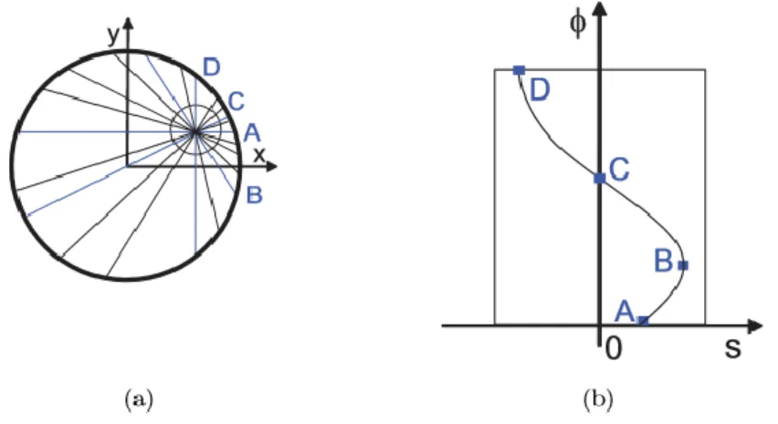
Sinograms are the most traditional way to represent data acquired in a PET scan. They are a histogram of the post-processed list-mode file (see Figure 3.2). The dimensions of a sinogram correspond to a distance s and an angle 𝜃. As seen in Figure 3.1, (s, 𝜃) coordinates pair describes the orientation of the LOR, where s is the tistance of a given LOR to the center of the FOV and 𝜃 is the angle between the LOR and the vertical axis. Evidently, the range of possible s’s and 𝜃’s is limited by the system’s geometry. Each entry in a sinogram is called a bin and has a value corresponding to the total amount of coincidences the detector pair described by the (s, 𝜃) has counted, hence being called a bin.

Figure 3.2: A centered point source and an off-centered point source in the scanner (a) describe, respectively, a straight line

and a sinusoidal line in the sinogram (b). Adapted from [10].

Mathematically, tracer distribution of an imaged object can be seen as a function with unknown density. A sinogram is the radon transform of that function. Imaging tracer distribution can be performed by applying the inverse Radon transform on the sinogram [11].

8

4 Image Reconstruction

When working with tomography techniques, image reconstruction is needed. This step takes the data acquired by the system and reconstructs it to obtain an image that best fits the object, as seen by the technique used. For instance, if one works with x-rays, the object is seen as regions that produce less or more attenuation to them. For ultrasounds, regions are seen as being more or less ultrasound reflective. However, PET differs from the later. Being an emission image technique, it relies on tracer presence throughout the internal organization of the object. As a result, the objective of PET image reconstruction is to image tracer distribution.

4.1 Image Reconstruction Algorithm

Image reconstruction algorithms are designed to fit the data they work with and the available computational power. At the very beginning, PET image reconstruction was based on analytical algorithms. These algorithms assume the data has little to no amount of noise, and their linear design and behavior forbids any complex image correction throughout the reconstruction process. However, with the ever-increasing computational power and acceleration techniques, iterative approaches to PET data reconstruction have appeared. Of most interest, statistic iterative algorithms, as these assume a better model for the Poisson noise distribution present in PET data, and can be shaped to incorporate noise reduction methods. The statistic algorithm exploited in this work was the Maximum Likelihood Expectation Maximization (ML-EM) algorithm. Although, we will be comparing the results obtained by this algorithm with Filtered Back Projection (FBP), for reasons that will be explained later on.

4.2 Iterative Algorithms and Expectation Maximization (EM)

As was previously mentioned, tracer distribution is a function with unknown density. Image reconstruction is used to obtain the cross-sectional image reflecting tracer distribution. The reconstruction algorithm of most relevance to this work is based on Expectation Maximization (EM) [12]. Through EM, tracer distribution is as follows:

𝐸[𝑝(𝜆)] = ∫ 𝑓(𝑥, 𝑦, 𝑧) ( 4.1 )

Where 𝐸[𝑝(𝜆)] is the probability expectation of a certain LOR, and 𝑓(𝑥, 𝑦, 𝑧) is the tracer spatial distribution.

With the improvements on computational power and capabilities, more complex image reconstruction algorithms are being implemented. Iterative algorithms have become more common, as they achieve better results. However, these expend more time, and require more computational power than analytical and recursive algorithms.

Iterative methods appear in the context of computational mathematics. These methods allow a sequence of improving approximate solutions, through successive forward and back projections on a given problem. Although an iterative algorithm may only converge to a non-absolute solution [13], it is preferable to use this approach when dealing with high complexity problems, as is the case of reconstructing PET data.

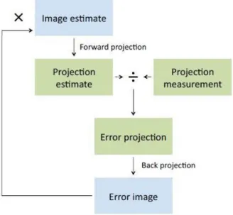
Most common algorithms for PET image reconstruction are based in the statistical Expectation Maximization (EM) approach, such as the ML-EM, Ordered Subset EM (OS-EM), or Maximum a Posteriori (MAP) [14]. An EM iteration comprises an Expectation and a Maximization phase. The flow chart for an iterative approach is depicted in Figure 4.1. In this case, the E-phase corresponds to a forward projection, where an estimated image is derived. Through the M-phase or back projection, an

9

error image is produced by comparing the estimated image with the actual measured data. The algorithm’s iteration ends by comparing the initial estimated image with the error image. The initial image estimate represents a non-zero distribution.

Figure 4.1: Schematic overview of an iterative Expectation Maximization (EM) reconstruction algorithm.

So as to obtain realistic results, there are five components that need be defined [15]: (1) a model for the image, (2) a model for the data, (3) a model for the physics of the measurement process, (4) a cost function, and (5) an algorithm to optimize the cost function.

The first (1) is the model for the activity distribution or object density. It represents the image 𝜆𝑗 to be

iterated throughout the image reconstruction process. The model for the data (2) takes into consideration the randomness of radioactive decay, by reflecting the statistical variation of PET data. For this component, it is considered that positron emission follows a Poisson distribution, so that the data collected is a collection of Poisson random variables. Next, a model for the physics of the measurement process (3) is needed, and this has been introduced as the system matrix. In Chapter 5 we will see how the LORs were calculated and system matrix assembled.

The cost or objective function (4) is the criterion used to determine which image is considered as the best estimate for the object. In the case of statistical algorithms, the cost function is a statistical function. Among these statistical approaches, one can distinguish the Bayesian from the classical methods. The Bayesian criteria for image estimation, such as the Maximum a Posteriori (MAP), assumes the unknown image is random and can be described by a probability density function known a priori. Among the classical criteria, there is the Maximum Likelihood, which is of great interest for this work and will be introduced next.

The final component is an algorithm to optimize the cost function (5). When working with Expectation Maximization, the general scheme for the iterative algorithm is displayed in Figure 4.1.

4.2.1 Maximum Likelihood Expectation Maximization (ML-EM)

The ML-EM algorithm has become the most common basis for PET data reconstruction approaches. The Maximum Likelihood criterion was first introduced by R. A. Fischer in 1921 [16]. Yet, it was only in 1982 that L.A. Shepp and Y. Vardi [17] introduced a new approach for emission tomography via combining the work of Fischer with a more recent work relating to EM [18]. Their approach took into consideration the Poisson distribution of emission tomography’s noise, thus taking into consideration

10

the characteristic lack of data in PET imaging. The ML-EM algorithm assumes that the quantity to estimate has unknown distribution [19]. Its equation is as follows:

𝜆_𝑗𝑛+1= 𝜆𝑗 𝑛 ∑ 𝑎𝑖 𝑖𝑗 ∑ 𝑦𝑖𝑎𝑖𝑗 ∑ 𝑎𝑗′ 𝑖𝑗′𝜆𝑗𝑛′ 𝑖 ( 4.2 )

Where 𝜆𝑛 _{and 𝜆}𝑛+1 _{represent the current image estimate and the image estimate that will result in the}

end of the 𝑛𝑡ℎ _{iteration, respectively. 𝑎 is the system matrix, and 𝑦 the PET data. The indexes 𝑖 and 𝑗}

represent the considered LOR and pixel, respectively. In Chapter 5, a practical example will be made to better illustrate how the algorithm works.

The preference of ML estimators, as the one used in the ML-EM algorithm, over other estimators, is based on two reasons related to the concept of bias and variance. ML estimators are asymptotically unbiased because, as the number of observations becomes large, the estimates become unbiased, that is, 𝐸[𝑝(𝜆)] → 𝜆. ML estimators are also asymptotically efficient because, for a large number of observations, they yield minimum variance, making the ML the estimator least susceptible to noise [20]. Even so, image reconstruction methods based on the ML estimation criterion, like the ML-EM, tend to yield noisy images. This happens since it is in the nature of this estimator to produce images consistent with the data. Since in emission tomography the data obtained is noisy, a good ML image estimate will also be a noisy image.

´The most common approach when dealing with the ML-EM algorithm is to allow a certain degree of bias in the reconstructed image. This is performed by finding the iteration at which the algorithm converges and, prematurely and intentionally, stop the ML-EM algorithm before it actually reaches the ML solution. Other approaches pass by explicitly implementing spatial smoothing in the images, by using filtering or Bayesian methods, which will be discussed later.

4.2.2 OS-EM and GPU Implementations

The main issue when designing an iterative approach to PET data reconstruction is the amount of data that must be dealt with. Alongside, time and computational power constraints lead to the development of algorithm optimizations. These range from developing different algorithms or by using the available software and hardware more efficiently.

A good example for an alternative to the ML-EM algorithm is the widely used OS-EM [21]. The Ordered Subset approach differs from its predecessor by dividing the data in non-overlapping groups. After, standard ML-EM is applied on each subset. Each iteration represents one go at each group, and the image estimate passes on from iteration to iteration. This algorithm is suitable when the data acquired is large enough. If it is not, or if too many subsets are considered, the noise will increase on the resulting reconstructed image.

Regarding using the available hardware more efficiently, efforts are being put to exploit GPU capabilities. GPUs are extremely useful when parallelizing scripted code. They easily surpass CPUs ability to deal with floating points operations [22]. This being, it is useful to parallelize certain parts of the image reconstruction code, as it greatly improves time performance. The main drawback is the code implementation. Lower level programming languages must be used, and the implementation is made to fit a specific GPU card. This means an implementation has reduced re-usage.

4.3 Filtered Back Projection (FBP)

Filtered Back Projection (FBP) is an analytic image reconstruction algorithm. The back projection step consists in tracing all the LORs in the spatial domain. Mathematically, FBP is the inverse radon

11

transform of the sinogram, which was introduced previously. By knowing the system’s geometry and having the data arranged in a sinogram manner, the inverse radon transform can be applied to produce the back projection image. However, the back projected image carries a great amount of noise. The main source for this noise comes from the loss of high frequencies when converting from the Fourier to the cartesian space [23]. The common procedure to contradict this effect is to convolute a filter with it, hence producing a Filtered Back Projection image.

Image reconstruction using FBP yields great results, if taken into consideration it is computationally inexpensive. However, even with filtering, this method continues to yield great amounts of noise, especially when dealing with the small statistics characteristic of PET technique. Yet, this is taken as the standard image reconstruction method and, therefore, will serve as a comparison to the image reconstruction algorithm developed in this work’s scope.

12

5 Data Correction and Regularization Methods

Images in Emission Tomography techniques are associated with high noise. The small data, photons interaction with matter, and hardware limitations, are the main factors for noise presence. Different noise reducing algorithms or quality enhancement approaches can be used to correct the data acquired, and preserve or enhance image quality. Exploiting different hardware’s capabilities can also contribute to noise reduction. Noise presence and overall image quality can be represented via signal-to-noise ratio (SNR) or through analysis of spatial resolution, among others.

5.1 Data Corrections

Data affecting events can be compensated through statistical approaches. Among these, some relate to the photons, such as: attenuation and scatter, TOF, and false coincidences. Hardware and reconstruction algorithms also affect noise presence by either reducing or incrementing it [7], [24].

5.1.1 Attenuation Correction

Taking into consideration photon attenuation enables correction of enclosed tissue regions which are falsely reconstructed with low activity. Photon intensity attenuation is given by:

𝐼(𝑥) = 𝐼0 𝑒µ𝑥

( 5.1 ) Where 𝐼(𝑥) is the intensity of the beam after traveling a distance 𝑥 in a given material with attenuation coefficient 𝜇. 𝐼0 is the initial beam intensity. By taking into account this effect, and using an attenuation

map, one can say that if a given LOR passes through more attenuating tissue, its corresponding pair of detectors should have, statistically, detected more coincidences. This correction is often used in human PET scans, where the detector’s size is considerable and there is significant tissue attenuation. The attenuation map is often a transmission image of the object, and represents an attenuation coefficient distribution map [8].

Figure 5.1: Representation of the effect caused by photon attenuation, with and without attenuation correction [25].

5.1.2 Time of Flight (ToF)

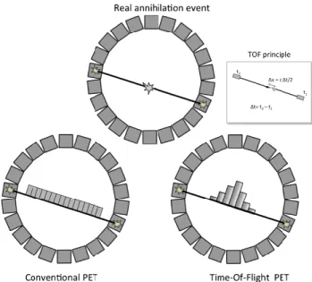
Time of flight is the precise measure of the time interval between the detection of both coincidence photons. By measuring this variable, we can obtain a better statistic distribution for the location of an event, as it indicates to which detector the event has occurred closer to (see Figure 5.2). This correction method requires hardware with high time resolution capabilities, with modern detectors having timing resolutions between 580-700 ps, sometimes as low as 300 ps [26].

13

Figure 5.2: Compared to conventional PET, the estimated ToF difference (∆𝑡) between the arrival times of photons on both

detectors in TOF-PET allows localization (with a certain probability) of the point of annihilation on the LOR. In TOF-PET, the distance to the origin of scanner (∆x) is proportional to the TOF difference via the relation ∆𝑥 =𝑐∆𝑡

2, where 𝑐 is the speed

of light, 𝑡1 the arrival time on the first detector, and 𝑡2 is the arrival time on the second detector [26].

5.1.3 False Coincidences – Scatter and Random Coincidences

Scatter events are responsible for activating detectors that do not include the initial photons directions. This leads to a mismatched LOR being considered. A common approach is to define a narrower energy window for the detected photons. As scatter results in the reduction of the photon’s energy, it is possible to reduce the contamination caused by this effect. In this case, the detector’s crystal should present good energy resolution capabilities.

Much like scatter events detection, random coincidences also produce mismatched LORs. However, limiting the energy window is not effective, as these coincidences can be produced by two unscattered photons. As is the case of TOF time resolution requirements, here goes the same. For a coincidence detection to be triggered, two detectors have to be paired. If the time interval between both triggers is too long, both photons do not belong to the same annihilation event. As can be seen in Figure 5.3, if the time interval between two detected photons is longer than the maximum time it would take the photon to cross the full FOV, then the coincidence is either random or results from a scatter event. Either way, the coincidence must be dismissed.

14

The hardware also takes a role in contributing to noise reduction. As was mention previously, detectors with high temporal and energy resolutions are useful when aiding in noise reduction. However, detectors have inherent problems related to their actuation and uniform behavior. The solutions for these problems appear, among others, as dead-time correction, and detector normalization [28].

5.1.4 System’s Geometry and Actuation

The dead-time is the time interval after a photon arrival in which a detector remains idle and cannot process other events. It results in smaller data counts and in the saturation of detectors. Knowing the dead-time inherent to a system allows the correction of saturated detectors, as these loose counts that would render them with much more statistic than those of unsaturated ones.

Detector normalization allows correction of LORs’ sensitivities. Sensitivity is affected due to the geometry of the system and hardware constraints [29]. In the first case, the angle to which a LOR intersects each of the detectors face. relative to the mean incident angle (see Chapter 5.1.5), strongly affects the sensitivity. The wider the detector’s face is, the more this effect can affect sensitivity. As for hardware constraints, the efficiency throughout all detectors is not always the same. In a block of detectors, there can exist a heterogeneous distribution of gains, which leads to sensitivity variability. In both cases, a full scan where all possible LORs are activated, can be performed. This method allows retrieving information on LOR sensitivity, and acquire the normalization coefficients for each LOR.

5.1.5 Depth of Interaction (DOI)

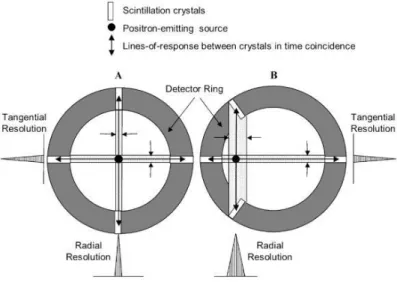
Lastly, one can have detectors able to measure the Depth of Interaction (DOI) [30]. The DOI is the point in the detector’s crystal where the photon interacted. This metric is possible through the double readout present in more advanced detectors, which allows the measurement of the asymmetry in the collected light at both ends of the detector’s readouts. As when tracing a LOR one would previously draw it from the middle point of both detectors face, the DOI error correction allows retracing LORs affected by this parallax error by adding information on photon detection. This way, it is possible to retrace the LOR in a more correct manner. Adding DOI correction into a system allows the improvement of radial resolution, as shown in Figure 5.4.

Figure 5.4: A) For a point source near the center of the FOV, photons enter crystals in the detector array through their very

small front faces and the difference between the LORs and the true photon flight paths is small, i.e. results in “good” radial resolution. B) For off-axis sources, photons can enter the crystals through their front faces and anywhere along their sides, so radial resolution is “poor”. Note that tangential resolution is not dependent on the DOI effect and is essentially constant across the FOV [31].

15

5.2 Data Regularization Methods

Preemptive noise reduction at machine and acquisition levels is very important. Still, although image reconstruction methods are designed to better fit the characteristics of the data and the user’s necessities, the statistics of PET data is often scarce, and image reconstruction will always carry noise. To minimize noise presence, quality enhancement methods are implemented throughout the image reconstruction step. These methods consist mostly on statistical approaches that aim to reduce noise by taking into consideration the local behavior on reconstructed images. What follows is an overview on how these methods actuate and the types that are of most interest to this work.

Figure 5.5: Noise presence in sources combined with poisson noise to demonstrate the noisy nature of PET imaging. The

images shown correspond to a) 10 counts per pixel; b) 100 counts per pixel; c) 1000 counts per pixel; d) 10000 counts per pixel.

5.2.1 Inter-Iteration Gaussian Filtering

Image filtering can be performed in the spatial or frequency domains. Filters are used to emphasize or remove certain image features, by performing smoothing, sharpening, and edge enhancement. Filters that operate in the frequency domain are of most use when dealing with frequency related problems, for example, removing the Mains Hum (power grid current frequency) from any data acquired with a system sensible to it.

Images can also be filtered in the spatial domain. This filtering approach consists in considering a neighborhood around a given pixel, so that its neighborhood has some weight on the new value for it. For each method, the dispersion and size of the neighborhood, as well as the weight given to it, must be decided. In this work, Gaussian filtering was considered.

Spatial Gaussian Filtering consists in using a Gaussian distribution as a “point-spread” function, which is achieved through convoluting it with the image. Since a pixelized image is a discretization of an object into pixels, a discrete approximation to the Gaussian function must be made. Since the Gaussian distribution is non-zero everywhere, its discretization would create an infinitely large convolution kernel. However, in practice, it is approximately zero at more than three standard deviations and this is often used as a kernel cut-off point [32].

5.2.2 Median Root Prior (MRP)

Other than using filters, image quality enhancement can be made based on a priori knowledge about the nature of the image. Such approaches guide the image reconstruction process into solutions considered more favorable. Among these, Bayesian inference is of great use. The logic behind Bayesian statistics states that the knowledge on prior events can be used to better predict future ones. In the case of image reconstruction, priors can be seen as the knowledge on the nature of the image. In the scope of this work, we will introduce the Median Root Prior.

The median root prior (MRP) [33] is based on the general assumption that an ideal PET image consists of constant neighborhoods with monotonous transitions between them. These are also the characteristics of the root signal of a median filter. A root signal remains unaltered when its corresponding filter is