Abstract—This paper proposes an appropriate activation
function for the fault classification decision algorithm. The decision algorithm based on the hybrid of discrete wavelet transform (DWT) and back-propagation neural network (BPNN) has been proposed to classify the fault type. The DWT is employed to decompose high frequency component of current signals. The maximum coefficient from the first scale at ¼ cycle of phase A, B, and C of post-fault current signals
and zero sequence current obtained by the DWT have been used as an input variable in a decision algorithm. The activation functions in each hidden layer and output layer have been varied, and the results obtained from the decision algorithm have been investigated with the variation of fault inception angles, fault types, and fault locations. The results have illustrated that the use of Hyperbolic tangent sigmoid function in the first and the second layers with Linear function in the output layer is the most appropriate scheme for the transmission system.
Index Terms—Neural Networks, Discrete Wavelet
Transform, Power Transformer
I. INTRODUCTION
RTIFICIAL neural networks (ANNs) techniques have
been proposed in some approaches in the literature to improve protective relay [1-9] due that these algorithms can give precise results. ANNs is characterized by (1) its pattern of connection between the neurons (called its architecture), (2) its method of determining the weights on the connections (called its training or learning algorithm), and (3) its activation function. Back-propagation neural network (BPNN) is a kind of neural networks, which is widely applied today owing to its effectiveness to solve almost all types of problem. Therefore, a decision algorithm, used for fault diagnosis in the power system to decrease complexity and duration of maintenance time, is required. Generally, the basic operation of an artificial neuron involves most units in neural networks transform their net input by using a scalar-to-scalar function called an "activation function", yielding a value called the unit's "activation". The activation function is sometimes called a
Manuscript received January 15, 2014.
N. Suttisinthong, and B. Seewirote are with Department of Electrical Engineering, Faculty of Engineering, Thonburi University, Bangkok 10160, Thailand (e-mail: [email protected], [email protected]).
A. Ngaopitakkul, and C. Pothisarn are with Department of Electrical Engineering, Faculty of Engineering, King Mongkut’s Institute of
Technology Ladkrabang, Bangkok 10520, Thailand (e-mail:
[email protected], [email protected]).
"transfer function". As a result, the activation function is a key factor in the artificial neural network structure. Back-propagation neural networks support a wide range of activation functions such as sigmoid function, linear function, and etc. The choice of activation function can change the behavior of the BPNN considerably. There is no theoretical reason for selecting a proper activation function. Hence, the objective of this paper is to investigate an appropriate activation function for the fault diagnosis decision algorithm. The activation functions in each hidden layers and output layer are varied, and the results obtained from the decision algorithm are studied.
The decision algorithm is a part of a transmission system scheme proposed in this paper. It is noted that the discrete wavelet transform is employed for extracting the high frequency component contained in the fault signals. The construction of the decision algorithm is detailed and implemented with various case studies based on Thailand electricity transmission and distribution systems.
II. SIMULATION
The ATP/EMTP is used to simulate fault signals at a sampling rate of 200 kHz. The fault types are chosen based on the Thailand’s transmission system as shown in Fig. 1. Fault patterns in the simulations are performed with various changes in system parameters as follows:
- Fault types considered in this study are : single line to ground (SLG : AG, BG, CG), double-line to ground (DLG : ABG, BCG, CAG), line to line (L-L : AB, BC, CA) and three-phase fault (3-P : ABC).
- Fault locations are varied from 10% to 90%, with the increase of 10% of the transmission line length measured from the bus MM3.
- Inception angle on a voltage waveform is varied between 0°-330°, with the increasing step of 30°. Phase A is used as a reference.
- Fault resistance is equal to 10 Ω
Fig. 1 The system used in simulation studies [1, 10].
Selection of Proper Activation Functions in
Back-propagation Neural Network algorithm
for Single-Circuit Transmission Line
N. Suttisinthong, B. Seewirote, A. Ngaopitakkul, and C. Pothisarn,
Member, IAENG
The fault signals generated using ATP/EMTP are interfaced to MATLAB for the fault detection algorithm. Fault detection decision [1, 7] is processed using the positive sequence current signals. The Clark’s transformation matrix is employed for calculating the positive sequence and zero sequence of currents. The mother wavelet daubechies4 (db4) [1, 4, 7, 9] is employed to decompose high frequency components from the signals. Coefficients obtained using the DWT of signals are then squared to clearly identify the abrupt change in the spectra. It is evident that the coefficients of high-frequency components are abruptly changed when a fault occurs, as shown in Fig. 2. The coefficients of scale 1 of DWT are used in the training processes for the neural networks in our case study.
Fig. 2 Wavelet transform from scale 1 to 5 for the positive sequence of current signal.
III. DECISION ALGORITHM
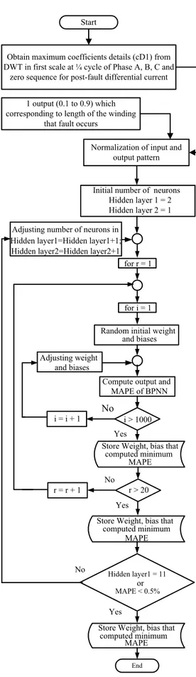
After the fault detection process, the coefficients detail of scale 1, which is obtained using the DWT, is used for training and test processes of the back-propagation (BPNN). In this paper, a structure of a BPNN consists of three layers which are an input layer, two hidden layers, and an output layer as shown in Fig. 3. Each layer is connected with weights and biases. In addition, the activation function is a key factor in the BPNN structure. The choice of activation function can change the behavior of the BPNN considerably. Hence, the activation functions in each hidden
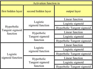
layers and output layer are varied as illustrated in Table 1 in order to select the best activation function. A training process was performed using neural network toolboxes in MATLAB which can be summarized in Fig. 4.
Table1 Activation functions in all hidden layers and output layers for training neural networks
Activation function in
first hidden layer second hidden layer output layer
Hyperbolic Tangent sigmoid function Logistic sigmoid function Linear function Logistic sigmoid Hyperbolic Tangent sigmoid
Hyperbolic Tangent sigmoid
function
Linear function Logistic sigmoid Hyperbolic Tangent sigmoid
Logistic sigmoid function Logistic sigmoid function Linear function Logistic sigmoid Hyperbolic Tangent sigmoid
Hyperbolic Tangent sigmoid
function
Linear function Logistic sigmoid Hyperbolic Tangent sigmoid
By observing Fig. 4, before the fault classification decision algorithm process, a structure of the BPNN consists of 4 inputs. The maximum coefficients detail (phase A, B, C and zero sequence of post-fault current) of DWT at the first peak time that can detect fault, is performed as input variables. The output variables of the BPNN for identifying fault types are designated as either 0 or 1, corresponding to phases A, B, C and ground (G). If each output value of BPNN is less than 0.5, no fault occurs on each phase; conversely, if this output value of BPNN is more than 0.5, a fault does occur. The output variables of the BPNN for locating the fault along the transformer windings are designated as values range of 0.1 to 0.9, corresponding to length of the winding that fault occurs. In addition, before training process, it is important to prepare the data before analysis because the obtained data will be clearly analyzed for the pattern between input pattern and output pattern. Input data sets define value range of 0 to 1 by normalization.
∑
f11 • 1 2 n 1 R P 1 , 1 1 , 1 iw • • 1 P 2 P 3 P 1 , 1 ,R S iw 1 f 1 f • • • 1 2 b
∑
1 1 1 S n 1 1 S b∑
1 1 1 n 1 1 b • • •∑
1 2 2 n 2 f • • • 2 2 b∑
1 2 2 S n 2 2 S b∑
1 2 1 n 2 1 b 1 2 a 1 1 S a 1 1 a 1 , 2 ,1 2S S lw 1 , 2 1 , 1 lw 2 f 2 f • • •∑
1 3 2 n 3 f • • • 3 2 b∑
1 3 3 S n 3 3 S b∑
1 3 1 n 3 1 b 2 2 a 2 2 S a 2 1 a 2 , 3 , 2 3S S lw 2 , 3 1 , 1 lw • • • 3 f 3 f 3 2 a 3 3 S a 3 1 a • • • LayerInput 1stHidden Layer 2ndHidden Layer Output Layer
Initial number of neurons
Store Weight, bias that computed minimum
MAPE Hidden layer1=Hidden layer1+1;
Store Weight, bias that computed minimum
MAPE Yes No
End Hidden layer1 = 11
or
MAPE < 0.5%
Adjusting weight and biases
Compute output and MAPE of BPNN
i = i + 1
No
Yes i > 1000
Store Weight, bias that computed minimum
MAPE Random initial weight
and biases for i = 1
r = r + 1 No
Yes r > 20 for r = 1 Hidden layer2=Hidden layer2+1 Adjusting number of neurons in
Hidden layer 1 = 2 Hidden layer 2 = 1 Obtain maximum coefficients details (cD1) from DWT in first scale at ¼ cycle of Phase A, B, C and
zero sequence for post-fault differential current Start
Normalization of input and output pattern 1 output (0.1 to 0.9) which
corresponding to length of the winding that fault occurs
Fig. 4. Flowchart for the training process
A training process for back-propagation neural network can be divided into three parts as follows [1]:
1. The feedforward input pattern, which has a propagation of data from the input layer to the hidden layer and finally to the output layer for calculating responses from input patterns illustrated in Equations 1 and 2.
(
)
(
2,1 1 1,1 1 2)
2 2
*
*f iw p b b lw
f
a = + + , (1)
(
3,2 2 3)
3
*
/p f lw a b
o ANN= + . (2)
where,
p is the input vector of ANNs
iw1,1 is the weights between input and the first hidden layer
lw2,1 is the weights between the first and the second hidden layers
lw3,2 is the weights between the second hidden layer and output layers
b1, b2 are the bias in the first and the second hidden layers respectively
b3 is the bias in output layers
f1, f2 are the activation functions (Hyperbolic tangent sigmoid function: tanh)
f3 is the activation function (Linear function)
2. The back-propagation for the associated error between outputs of neural networks and target outputs; the error is fed to all neurons in the next lower layer, and also used to an adjustment of weights and bias.
3. The adjustment of the weights and bias by Levenberg-Marquardt (trainlm). This process is aimed at trying to match between the calculated outputs and the target outputs. Mean absolute percentage error (MAPE) as an index for efficiency determination of the back-propagation neural networks is computed by using Equation 3.
% 100 * /
/ /
* 1
1
∑
=
− =
n
i TARGETi
TARGETi ANNi
p o
p o p
o n
MAPE (3)
where, n is the number of test sets.
During training process, the weight and biases are adjusted by Levenberg-Marquardt (trainlm), and there are 20,000 iterations in order to compute the best value of MAPE. The number of neurons in both hidden layers is increased before repeating the cycle of the training process. The training procedure is stopped when reaching the final number of neurons for the first hidden layer or the MAPE of test sets is less than 0.5%.
0 10 20 30 40 50 60 70 80 90 100 80
85 90 95 100 105 110 115 120
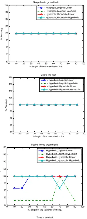
Single line to ground fault
% length of the transmission line.
%
A
c
c
u
ra
c
y
Hyperbolic,Logistic,Linear Hyperbolic,Logistic,Hyperbolic Hyperbolic,Hyperbolic,Linear Hyperbolic,Hyperbolic,Hyperbolic
0 10 20 30 40 50 60 70 80 90 100 80
85 90 95 100 105 110 115 120
Single line to ground fault
% length of the transmission line.
%
A
c
c
u
ra
c
y
Logistic,Logistic,Linear Logistic,Logistic,Hyperbolic Logistic,Hyperbolic,Linear Logistic,Hyperbolic,Hyperbolic
0 10 20 30 40 50 60 70 80 90 100 80
85 90 95 100 105 110 115 120
Line to line fault
% length of the transmission line.
%
A
c
c
u
ra
c
y
Hyperbolic,Logistic,Linear Hyperbolic,Logistic,Hyperbolic Hyperbolic,Hyperbolic,Linear Hyperbolic,Hyperbolic,Hyperbolic
0 10 20 30 40 50 60 70 80 90 100 80
85 90 95 100 105 110 115 120
Line to line fault
% length of the transmission line.
%
A
c
c
u
ra
c
y
Logistic,Logistic,Linear Logistic,Logistic,Hyperbolic Logistic,Hyperbolic,Linear Logistic,Hyperbolic,Hyperbolic
0 10 20 30 40 50 60 70 80 90 100
80 85 90 95 100 105 110 115 120
Double line to ground fault
% length of the transmission line.
%
A
c
c
u
ra
c
y
Hyperbolic,Logistic,Linear Hyperbolic,Logistic,Hyperbolic Hyperbolic,Hyperbolic,Linear Hyperbolic,Hyperbolic,Hyperbolic
0 10 20 30 40 50 60 70 80 90 100 80
85 90 95 100 105 110 115 120
Double line to ground fault
% length of the transmission line.
%
A
c
c
u
ra
c
y
Logistic,Logistic,Linear Logistic,Logistic,Hyperbolic Logistic,Hyperbolic,Linear Logistic,Hyperbolic,Hyperbolic
0 10 20 30 40 50 60 70 80 90 100
70 75 80 85 90 95 100 105 110 115 120
Three phase fault
% length of the transmission line.
%
A
c
c
u
ra
c
y
Hyperbolic,Logistic,Linear Hyperbolic,Logistic,Hyperbolic Hyperbolic,Hyperbolic,Linear Hyperbolic,Hyperbolic,Hyperbolic
0 10 20 30 40 50 60 70 80 90 100
80 85 90 95 100 105 110 115 120
Three phase fault
% length of the transmission line.
%
A
c
c
u
ra
c
y
Logistic,Logistic,Linear Logistic,Logistic,Hyperbolic Logistic,Hyperbolic,Linear Logistic,Hyperbolic,Hyperbolic
(a) Hyperbolic in first hidden layer (b) Logistic in first hidden layer
0 10 20 30 40 50 60 70 80 90 100 90
92 94 96 98 100 102 104 106 108 110
Average accuracy of fault types in transmission lines
% length of the transmission line.
%
A
c
c
u
ra
c
y
Hyperbolic,Logistic,Linear Hyperbolic,Logistic,Hyperbolic Hyperbolic,Hyperbolic,Linear Hyperbolic,Hyperbolic,Hyperbolic
0 10 20 30 40 50 60 70 80 90 100 90
95 100 105 110
Average accuracy of fault types in transmission lines
% length of the transmission line.
%
A
c
c
u
ra
c
y
Logistic,Logistic,Linear Logistic,Logistic,Hyperbolic Logistic,Hyperbolic,Linear Logistic,Hyperbolic,Hyperbolic
(a) Hyperbolic in first hidden layer (b) Logistic in first hidden layer
Fig. 6. Comparison of average accuracy when identifying the fault type at various lengths of the transmission line among various activation functions.
IV. CONCLUSION
In this paper, study of an appropriate activation function for the decision algorithm used in the transmission system has been discussed. The fault classification decision algorithm can be classified the fault type and fault location using the back-propagation neural networks (BPNN). The maximum coefficient from the first scale at ¼ cycle of phase
A, B, and C of post-fault current signals and zero sequence current obtained by the DWT have been used as an input variable in a decision algorithm. The activation functions in each hidden layer and output layer have been varied, and the results obtained from the decision algorithm have been investigated with the variation of fault inception angles, fault types, and fault locations. The results have illustrated that the use of Hyperbolic tangent sigmoid function in the first and the second layers with Linear function in the output layer is the most appropriate scheme for the transmission system.
ACKNOWLEDGMENT
This work is partially supported by the King Mongkut’s Institute of Technology Ladkrabang Research fund. The authors would like to thank for this financial support. The authors would like also to gratefully acknowledge the helpful comments and suggestions of the reviewers, which have improved the presentation.
REFERENCES
[1] P. Chiradeja and A. Ngaopitakkul, “Identification of Fault Types for Single Circuit Transmission Line using Discrete Wavelet transform and Artificial Neural Networks,” In Proceedings of 2009
International Conference on Electrical Engineering (ICEE2009), pp. 1520-1525, 2009.
[2] N. Perera, A.D. Rajapakse, “Recognition of Fault Transients Using a Probabilistic Neural-Network Classifier,” IEEE Trans-actions on Power Delivery, Vol. 26, No. 1, pp. 2011, 410 – 419.
[3] D. Barbosa, D.V. Coury, and M. Oleskovicz, “New approach for power transformer protection based on intelligent hybrid sys-tems,” IET Generation, Transmission & Distribution., Vol. 6, No. 10, 2012, pp. 1009-1018.
[4] A. Ngaopitakkul, C. Jettanasen, J. Klomjit, C. Pothisarn, B. Seewirote, and N. Suttisinthongn, “Application of back-propagation neural network for transformer differential protection schemes part 1 discrimination between external short circuit and internal winding fault,” Joint 6th International Con-ference on Soft Computing and Intelligent System (SCIS) and 13th International Symposium on Advanced Intelligent Systems, 2012, pp. 1493-1498.
[5] Yang Cunxiang, Bao Hao, “The fault diagnosis of transformer Based on the SOM neural network current,” Proceedings of the 5th Conference on Measuring Technology and Mechatronics Automation, 2013, pp. 1178-1180.
[6] S. Seyedtabaii, “Improvement in the performance of neural network-based power transmission line fault classifiers,” IET – Generation, Transmission and Distribution, Vol. 6, No. 8, pp. 731-737, 2012. [7] A. Ngaopitakkul and C. Jettanasen, “Combination of Discrete
Wavelet Transform and Probabilistic Neural Network Algorithm for Detecting Fault Location on Transmission System,” International Journal of Innovative Computing, Information and Control, Vol. 7, No. 4, pp. 1861-1874, 2011.
[8] Y.Zhang, X.Ding, Y.Liu and P.J. Griffin, “An artificial neural network approach to transformer fault diagnosis”, IEEE Trans. Power Delivery, Vol. 11, No. 4, pp. 1836-1841, 1996.
[9] A. Ngaopitakkul and A. Kunakorn, “Internal Fault Classification in Transformer Windings using Combination of Discrete Wavelet Transforms and Back-propagation Neural Networks,” International Journal of Control, Automation, and Systems (IJCAS), Vol. 4, No. 3, pp. 365-371, June 2006.
![Fig. 1 The system used in simulation studies [1, 10].](https://thumb-eu.123doks.com/thumbv2/123dok_br/16388060.192457/1.892.470.819.1003.1125/fig-used-simulation-studies.webp)