REVISTA BRASILEIRA DE ECONOMIA ISSN 1806-9134 (online) FUNDAÇÃO GETULIO VARGAS
New Tools for the CGE Analysis of PTAs in the
era of Non-Tariff Barriers and Global Value
Chains: The Case of Mercosur and China
Lucas P. do C. Ferraz* Marcel B. Ribeiro*
Contents
1 Introduction. . . 330
2 Contextualizing Brazilian economy in the era of global value chains . . . 333
3 The “Natural Trade Partner” concept extended to Trade in Intermediates. 337
4 Estimating the Ad valorem equiva-lents of TBT/SPS measures . . . 340
5 Database and Empirical Results . . . 343
6 Case Study . . . 347
7 Final Remarks. . . 355
Keywords
Non-tariff barriers, Global Value Chains, Preferential Trade Agreements JEL Codes
F14, C01, C68
Abstract·Resumo
This article explores new tools for the ex-ante analysis of PTAs using large scale CGE models. The traditional impact analysis based on tariff cuts and gross trade performance is then extended to incorporate new features of the ongoing globalization process, such as non-tariff barriers (NTBs) and the so-called trade in value-added. Several methodological as well as conceptual issues are then readdressed, including the proper use of estimated ad-valorem equivalents of NTBs as inputs in perfect competition CGE models as well as the very concept of a “preferential trade partner” in a world where nearly 65% of global exports correspond to trade in intermediates. The article concentrates its impact analysis on the Brazilian economy—providing an overview of its trade policy over the last decades—and the likely consequences of a hypothetical PTA involving Mercosur and China.
1. Introduction
International trade governance and the very nature of trade have changed significantly over the last decades. First, the difficulties faced by the multilateral trade system at the WTO prompted the escalation of preferential trade agreements (PTA’s) at the bilateral, regional and even plurilateral levels. Just over the last two decades, more than four hundred PTAs were notified. Second, countries have been progressively trading in tasks (Grossman
& Rossi-Hansberg,2008) instead of trading in goods. Nowadays, more than two-thirds
of global exports correspond to trade in intermediate goods and services, reflecting the increasing relevance of the fragmentation of production (Baldwin & Lopez-Gonzalez,2013;
Daudin, Rifflart & Schweisguth,2011). Last, but not least, the so called “non-tariff barriers”
have gained prominence in a world of much lower import tariffs. More recently, countries
*Escola de Economia de São Paulo, Fundação Getúlio Vargas (EESP/FGV). Rua Itapeva, 474, Bela Vista, São Paulo, SP, Brasil. †[email protected] [email protected]
This is an open-access article distributed under the terms of the Creative Commons Attribution License.
Rev. Bras. de Econ. Vol. 72, No. 3 (Jul–Set 2018) 330–360 330
notifications of technical barriers to trade (TBTs), as well as sanitary and phytosanitary measures (SPSs) started to proliferate, raising serious concerns among policymakers of potential protectionist behavior by countries, possibly threatening global efforts towards free trade. Regardless of the real objectives of the imposition of non-tariff barriers such as TBTs and SPSs, several empirical studies have pointed out their likely negative effects on trade flows (Leamer,1990;Moenius,2004;Disdier, Fontagné & Mimouni,2008;Kee, Nicita &
Olarreaga,2009;Ferraz, Ribeiro & Monastério,2017). These new features of globalization
have obviously posed new challenges for the economic evaluation of preferential trade arrangements.
In this paper, we first contextualize the economy of Brazil into this new and challenging global environment. A comprehensive data set comprised of global input-output tables such as TIVA (Trade in Value Added), WIOD (World Input-Output Database) and GTAP (Global Trade Analysis Project) is used, conveying detailed information on how the economy of Brazil is currently positioned in terms of its integration into regional/global value chains. Particular emphasis is given to the manufacturing sector, once this is often considered to be a key sector for developing economies and it is usually the sector with the greatest potential for integration into relevant international supply chains. The second part of the paper is devoted to a specific case study where the possible implications of a “new age”1preferential
trade agreement between Brazil and China2is evaluated. China is currently one of Brazil’s
most relevant “natural trade partners” (Venables,2003;Ferraz,2012). A set of dynamic CGE simulations is carried out where the results are evaluated according to the logic of integration to international supply chains as well as trade in value added, instead of the usual ‘gross” trade analysis. In this sense, we explore an innovative approach to evaluate the economic impacts of PTAs in an increasingly interconnected global economy. In both parts of the paper, we draw extensively on the recent input-output framework developed
byJohnson & Noguera(2012a,2012b) and extended byKoopman, Wang & Wei(2014) to
evaluate trade in value added.
The methodological approaches taken in this paper offer original contributions both to the empirical literature of PTAs as well as to the literature of Gravity models applied to the estimation of non-tariff barriers, such as TBT and SPS. Regarding PTAs, the existing literature is extensive and draws on the early theoretical works of Jacob Viner (1950), James Meade (1955) and Lipsey (1957) among others. Those authors were the first to formalize the concepts of trade creation and trade diversion in a preferential trade arrangement. A very important development of this literature derives from the empirical works with gravity models (Anderson,1979), where the definition of a “natural trade partner” has its origins. This paper extends the concept of a “natural trade partner” to a world economy currently interconnected through international supply chains. The extended concept traces out “backward” and “forward” linkages of trade in intermediates among countries, shedding some light on those potential trade partners where the formation of PTAs is more prone to lead to integration according to the value chain logic. This paper also offers methodological alternatives to a relatively recent empirical literature on the role of PTAs to the formation of global/regional value chains (Blyde, Graziano & Martincus,2015;Orefice & Rocha,2011;
1In the so called “new age” trade agreements, trade talks on regulatory harmonization and mutual recognition are at the center stage (seeHertel, Walmsley & Itakura,2001).
Hayakawa & Yamashita,2011). Based on the results of varying econometric approaches, these authors find a positive correlation between the formation of PTAs and the integration of international production chains. However, problems associated with endogeneity and the fact that not all trade flows and foreign direct investments generated by PTAs are related to the formation of global/regional value chains do not allow this literature to come up with safe conclusions regarding causality. The dynamic CGE approach adopted in this work seems more suitable to handle the methodological drawbacks of this recent empirical literature since the simulation of a PTA can be taken as an exogenous shock. Moreover, interregional CGE models—such as the one used in this work3—are generally based on
sufficiently detailed global input-output databases, where trade in value added as well as trade in intermediates can be traced out through the use of appropriate input-output techniques (Johnson & Noguera,2012a).
Regarding Gravity models, we estimate the ad valorem equivalents of non-tariff barriers (TBT/SPS) to be used in a consistent way as inputs into perfect competition CGE models. Most of the empirical literature available on the effects of TBT/SPS measures on bilateral trade flows are based on gravity models. However, existing misspecification problems in several of these studies called the attention of a group of trade theorists, starting by the influential work ofAnderson & van Wincoop(2003), where the issue of “remoteness” in gravity equations was first addressed. The work by Silva & Tenreyro(2006) pointed out to another possible misspecification problem in gravity regressions, suggesting that under heteroskedasticity, the parameters of log-linearized gravity models estimated by OLS may lead to biased estimates of the true elasticities. More recently, another influential work byHelpman, Melitz & Rubinstein(2008) raised the issue on the existence of firm heterogeneity and also on the correct treatment of zero bilateral trade flows in traditional gravity estimations, prompting a new generation of empirical studies addressing those new specification concerns. Some recent examples include the works ofDisdier & Marette
(2010),Crivelli & Groeschl(2016) andFerraz et al.(2017).
In our case study, we adopt a rather sophisticated estimation approach, based on the new insights fromHelpman et al.(2008). Their approach seems more suitable to our case study since it can discriminate between the effects of TBT/SPS measures on the extensive (industry’s fixed costs) as well as the intensive (industry’s variable costs) margins of trade, according to the new insights on the heterogeneity of exporting firms described in the seminal work byMelitz(2003).
Our final results highlight three important singularities. First, the economy of Brazil is far from the ongoing global paradigm of specialization in stages of production (fragmen-tation) and connection to global/regional value chains. On the contrary, the low levels of foreign content embedded in Brazilian manufacturing exports are suggestive that they are still mostly “made in Brazil”, whereas global exports are progressively “made in the world”. Second, TBTs and SPSs measures may constitute significant bilateral trade barriers among Brazil and China. Ignoring the existence of those barriers can significantly undermine sector-specific gains from trade if PTA negotiations are restricted to the reduction of traditional GATT (General Agreement on Tariffs and Trade) instruments such as import tariffs and quotas. Third, joining a PTA with China may pave the way to the integration of Brazil’s manufacturing sector to relevant GVCs in more dynamic regions of the world.
The structure of this paper is organized as follows.Section 2presents a set of stylized trade facts about the Brazilian economy, exploring some of the new information available in the “so called” TIVA and WIOD databases. Section 3discusses the extended concept of “natural trade partners” according to the logic of global/regional value chains. Sections 4 describes the econometric model used to estimate thead valoremequivalents of existing TBTs and SPSs measures on bilateral trade flows between Brazil and China. Section 5
presents the database for the econometric estimations. Section 6shows the impacts of a PTA involving Mercosur and China, under alternative scenarios, tracing out bilateral trade in value added as well as bilateral trade in intermediates.Section 7summarizes the main findings of this paper.
2. Contextualizing Brazilian economy in the era of global value chains
From the post second world war till the end of the eighties, the import substitution model formed the basis of industrialization policies in Latin American countries, including Brazil.Brazil’s import substitution model succeeded in building a diversified and complex domestic manufacturing sector, based on a relatively dense and interconnected domestic supply chain of intermediates and final goods. By the beginning of the eighties, value added in manufacturing activities in Brazil peaked 25% of country’s GDP, a level close to the average of OECD countries at the time. The significant development of manufacturing activities in Brazil was followed by widespread productivity gains over the domestic economy. Along two decades, from 1960 to 1980, average annual growth in total factor productivity in Brazil reached 2.3%, a level by far the highest among Latin American countries, and also higher than in the USA, South Korea, China and the average of OECD countries during the same period (Veloso, Matos & Coelho,2015).
The end of the seventies and beginning of the eighties were characterized by a period of market-oriented reforms in China and the start of its emergence as a global trader. Far from the adoption of the import substitution model, China and most of its Asian neighbors took advantage of their cheaper labor costs and decided to unilaterally open up to trade, attracting a whole set of less sophisticated manufacturing activities from richer offshoring nations such as the USA and Western European countries. This period also coincided with the decline of the share of manufacturing value added over GDP in most developed regions in the world as well as in some developing countries such as Brazil: in 1984, manufacturing valued added represented near 23% of GDP in OECD countries and Brazil. In 2010, this share had declined to less than 15% in both regions. Along the same period, the share of manufacturing value added over GDP in Asia raised from 22% to over 28% in 2010 (Bonelli
& Bacha,2013). Those facts may help to explain why the Asian continent is nowadays called
“factory Asia”.
The emergence of Asia as a significant pole of manufacturing activity4in the world gave
rise to a new global pattern of trade specialization: developed regions became relatively more specialized in the production and supply of high-skilled services as well as some high-tech intermediate goods whereas developing regions became relatively more specialized in the
production and supply of low-skilled manufacturing tasks. Despite its higher concentration in the international trade of intermediates instead of final goods5, this new global pattern of
specialization seems to be in agreement with Hecksher–Ohlin predictions regarding trade patterns based on factor proportions theory (Los, Timmer & De Vries,2015).
The new global pattern of specialization can be easily identified in the numbers shown in
Table 1for a set of regions over the period 1995–2008, working with the data sourced from
WIOD. Using a similar methodology as the one adopted byTimmer, Los, Stehrer & De Vries
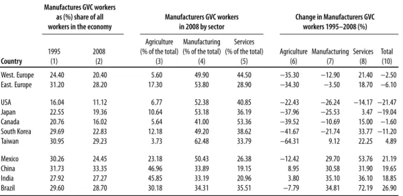
(2013), it is possible to trace out the number of workers directly and indirectly involved in the production of final manufacturing goods in each region. Results inTable 1highlight four important facts. First, manufacturing related jobs have been shrinking as a share of total labor force for all countries and regions presented, except China (columns 1 and 2). Second, over 50% of manufacturing related jobs is not directly involved in manufacturing activity. Instead, they are indirectly involved through agriculture and services activities. In Brazil, nearly 65% of manufacturing related jobs are actually employed out of the manufacturing sector (columns 3 and 5). Third, direct manufacturing jobs have been losing participation in developed regions’ labor force. On the other hand, they have been gaining relative importance in developing ones (column 7). Fourth, the production of final manufactured goods has become more intensive in services for all regions in the world. However, this process has been clearly more intensive in developed regions compared to developing ones (columns 6, 7 and 8).
Regardless of being a developing economy, structural changes in Brazil are harder to interpret based solely on the information available inTable 1. On one hand, direct manufacturing employment has increased over the period 1995–2008 in Brazil, as in other developing regions such as Mexico, China and India. On the other hand, the growth of manufacturing related service jobs in Brazil has increased nearly two times faster, a pattern
Table 1.GVC workers directly and indirectly involved in the production of manufacturing goods (1995–2008).
Manufactures GVC workers as (%) share of all workers in the economy
Manufacturers GVC workers in 2008 by sector
Change in Manufacturers GVC workers 1995–2008 (%)
Country
1995 (1)
2008 (2)
Agriculture (% of the total)
(3)
Manufacturing (% of the total)
(4)
Services (% of the total)
(5)
Agriculture (6)
Manufacturing (7)
Services (8)
Total (10) West. Europe 24.40 20.40 5.60 49.90 44.50 −35.30 −12.90 21.40 −2.50 East. Europe 31.20 28.20 17.30 53.80 28.90 −34.30 −3.50 18.70 −6.10
USA 16.04 11.12 6.77 52.38 40.85 −22.43 −26.24 −14.17 −21.47
Japan 22.55 19.36 10.64 53.18 36.19 −37.96 −25.53 3.47 −19.04 Canada 20.76 16.02 5.64 41.00 53.36 −39.52 −10.69 15.00 −1.60 South Korea 29.69 22.83 12.18 49.20 38.62 −41.67 −21.74 33.77 −11.20
Taiwan 30.95 29.23 3.73 62.48 33.79 −64.31 9.12 22.25 4.89
Mexico 30.26 24.45 23.18 50.43 26.38 −12.42 29.70 53.76 21.19
China 31.73 33.35 46.96 33.89 19.15 8.95 30.58 31.90 19.65
India 27.92 27.27 45.85 33.19 20.96 3.80 35.10 36.10 18.85
Brazil 29.60 28.70 30.18 34.31 35.51 −7.79 34.81 72.19 26.90
Source:Author’s calculation based on World Input-Output Database.
of specialization that resembles the ones verified for the group of developed regions in the world. Indeed, a broader view of structural changes occurred in the Brazilian economy for the period of 1984–2014 reveals that the share of services value added raised from 45% of country’s GDP to nearly 70%. Regarding the composition of its total exports, in 2011 manufactured and services exports corresponded to 41.4% and 16.2% of total exports in Brazil, respectively. However, when the composition of total value added exported is taken into consideration, those same shares change to 27.4% and 40.7%, suggesting that a lot of services intermediates are exported embedded in the exports of manufactured goods.
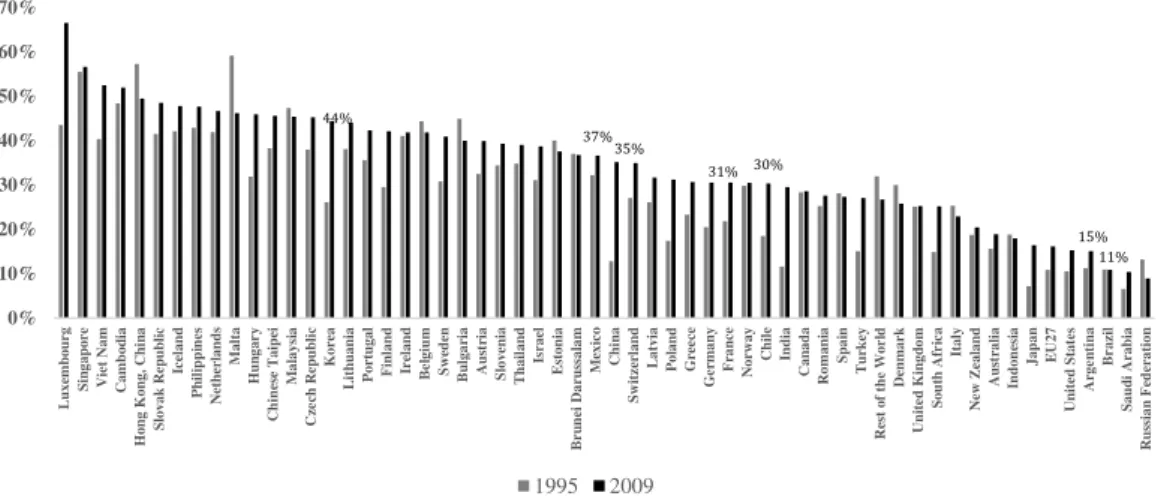
Therefore, the ongoing pattern of specialization in services activities for the economy of Brazil, rather than the result of deeper integration to global/regional value chains, as it seems to be the case for developed economies (Table 1), may be rather the consequence of its relative isolation. Excessive import protection for long periods, associated with the formalization of just a few and usually shallow PTAs over the last decades, might have contributed to the current low competitiveness of Brazil’s manufacturing sector and its weak participation in relevant international supply chains.Figure 1shows the evolution of the foreign content embedded in manufactured exports for a group of 58 countries, from 1995 to 2009. While most countries in the sample seemed to have significantly increased its participation in the ongoing process of fragmentation of production over the period, the share of foreign intermediates embedded in Brazil’s manufactured exports has kept stagnated at the level of 11%. According to this criterion, the manufacturing sector in Brazil is one of the least integrated to value chains among its peers, showing a higher level of integration only in comparison to the manufacturing sectors in commodity exporters such as Saudi Arabia and Russia.
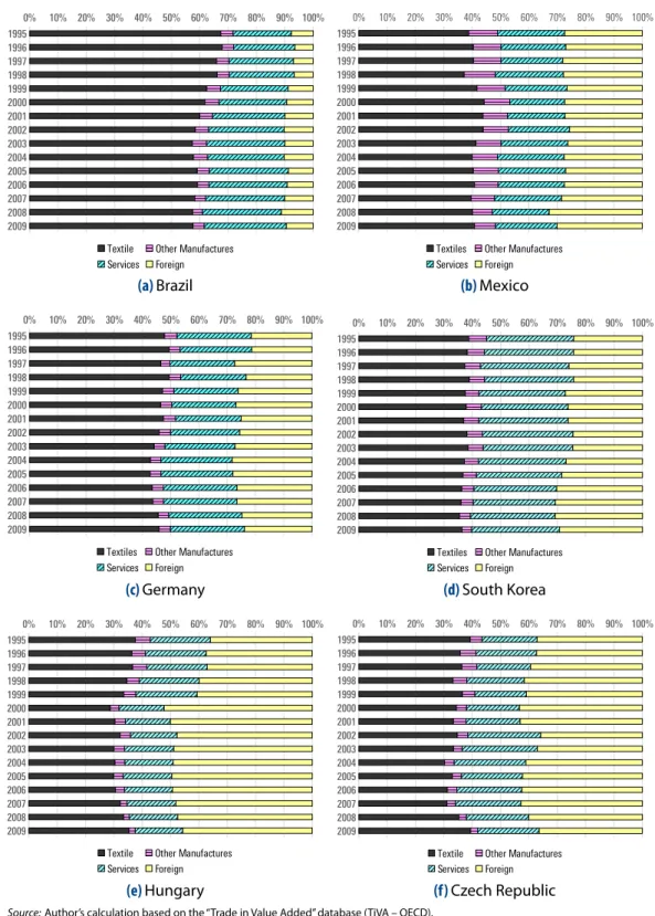
Figure 2slices up the total value added created in the production of a final good in the
textile sector for a sample of countries, including Brazil, over the period 1995–2009.6This
analysis unravels two main facts. First, a significant share of total value added generated in the production of a final textile good remunerates factors of production in the domestic services sector. This is true for all countries in the sample. Second, there is a significant
44% 37% 35% 31% 30% 15% 11% 0% 10% 20% 30% 40% 50% 60% 70% L u xe m b ou rg S in gap or e Vie t N am Cam b od ia Hon g Kon g, Chi n a S lovak Re p u b li c Ic elan d P h il ip p in es Ne th er lan d s M alt a Hu n gar y Chi n es e T aip ei M alays ia Cz e ch Re p u b li c Kore a L it h u an ia P or tu gal F in lan d Ir elan d B e lgiu m S we d en B u lgaria Aus tr ia S loveni a T h ail an d Is rae l E st on ia B r u n ei Dar u ss alam M exic o Chi n a S wit z er lan d L at via P ol an d Gre e ce Ger m an y F ran ce Nor
way Chile India
Canad a Rom an ia S p ai n T u rk ey Re st of t h e Wor ld De n m ar k Uni te d Ki n gd om S ou th Af r ic a It aly Ne w Z e al an d Aus tr ali a In d on es ia Jap an E U27 Uni te d S tat es Ar ge n tin a B r az il S au d i Ar ab ia Rus sian F ed er at ion 1995 2009
Source:Author’s calculation based on the “Trade in Value Added” database (TiVA – OECD).
Figure 1.Foreign content in manufacturing exports over the period 1995–2009.
1995 1996 1997 1998 1999 2000 2001 2002 2003 2004 2005 2006 2007 2008 2009
0% 10% 20% 30% 40% 50% 60% 70% 80% 90% 100%
Textile OtherManufactures Services Foreign
(a)Brazil
1995 1996 1997 1998 1999 2000 2001 2002 2003 2004 2005 2006 2007 2008 2009
0% 10% 20% 30% 40% 50% 60% 70% 80% 90% 100%
Textiles OtherManufactures Services Foreign
(b)Mexico
1995 1996 1997 1998 1999 2000 2001 2002 2003 2004 2005 2006 2007 2008 2009
0% 10% 20% 30% 40% 50% 60% 70% 80% 90% 100%
Textiles OtherManufactures Services Foreign
(c)Germany
1995 1996 1997 1998 1999 2000 2001 2002 2003 2004 2005 2006 2007 2008 2009
0% 10% 20% 30% 40% 50% 60% 70% 80% 90% 100%
Textiles OtherManufactures Services Foreign
(d)South Korea
1995 1996 1997 1998 1999 2000 2001 2002 2003 2004 2005 2006 2007 2008 2009
0% 10% 20% 30% 40% 50% 60% 70% 80% 90% 100%
Textile OtherManufactures Services Foreign
(e)Hungary
1995 1996 1997 1998 1999 2000 2001 2002 2003 2004 2005 2006 2007 2008 2009
0% 10% 20% 30% 40% 50% 60% 70% 80% 90% 100%
Textile OtherManufactures Services Foreign (f)Czech Republic
Source:Author’s calculation based on the “Trade in Value Added” database (TiVA – OECD).
foreign content embedded in the local production of a final textile good for all countries in the sample, except Brazil. For instance, in 2009 nearly 30% of total value added created in the production of a final textile good in Germany was devoted to the payment of factors of production located abroad. For the same year, this share was nearly 10% in Brazil.
When the whole domestic economy is considered, calculated shares inFigure 3confirm that nearly 87% (in average) of all inputs used in the production of a final manufactured good in Brazil (in 2011) were sourced locally. It is worthy to note the relevance of China as a significant source of imported intermediates.
The analysis of Figures1to3suggests that the manufacturing sector in Brazil is still little integrated to significant international supply chains. The flipside of this whole process seems to be the increasing relevance of lower value-added services activities in Brazil and the resulting fall in total factor productivity.
3. The “Natural Trade Partner” concept extended to Trade in
Intermediates
Assuming that PTAs can create additional incentives for member countries to integrate their production structures and to build global/regional value chains, which partners should a country prioritize once it has decided to open up to trade?
One possible way to tackle this issue is to measure the participation of a country in international supply chains according to its “backward” and “forward” linkages (Koopman
et al.,2014). On one hand, the higher the foreign content embedded in a country’s domestic
exports, the stronger are its backward linkages. By the same token, the higher the share of
Agriculture,Hunting,ForestryandFishing MiningandQuarrying Food,BeveragesandTobacco TextilesandTextileProducts Leather,LeatherandFootwear WoodandProductsofWoodandCork Pulp,Paper,Paper,PrintingandPublishing Coke,RefinedPetroleum andNuclearFuel
ChemicalsandChemicalProducts RubberandPlastics OtherNon-MetallicMineral BasicMetalsandFabricatedMetal Machinery,Nec ElectricalandOpticalEquipment TransportEquipment Manufacturing,Nec Services
0.0% 20.0% 40.0% 60.0% 80.0% 100.0%
86.7% 86.1%
95.5% 88.2%
91.0% 93.8% 88.5% 81.5%
83.0% 80.4%
89.0% 84.4%
85.7% 73.6%
83.1% 88.6%
91.0%
ROW NAFTA KOR JPN E27 CHINA BRAZIL
Source:Author’s calculation based on World Input-Output Database.
a country’s domestic exports of intermediates embedded in third countries’ exports, the stronger its forward linkages.
Therefore, the formalization of PTAs among countries with pre-existing strong back-ward and forback-ward linkages should be more prone to the formation of global/regional value chains, as long as it may reinforce bilateral trade in intermediates, once trade barriers are reduced.7
The Chinese economy is responsible for more than 20% of Brazilian imports and exports and can then be considered a Brazil’s natural trade partner, according to Vinner’s traditional definition. When backward and forward linkages are considered,Figure 4and5show that China is also a significant source of intermediates to Brazil’s exports (backward linkages) as well as a significant consumer of Brazil’s exports of intermediate goods that go embedded in Chinas’s exports (forward linkages) to third countries.
Therefore, a PTA involving Brazil and China may have a high potential to be welfare improving (net trade creation) for the Brazilian economy and may also increase bilateral trade in intermediates according to the supply chain logic. Backward and forward linkages, therefore, can extend the traditional view of a natural trade partner beyond trade creation and trade diversion to include how prone is a hypothetical PTA to create additional price/cost incentives to the formation of global/regional supply chains.
Figure 4and5also suggest that other regions of the world such as NAFTA and EU_27
could possibly be considered natural trade partners for Brazil, according to the value chain logic.8 However, when an intertemporal perspective is taken into consideration, China
seems to take the lead as a preferential trade partner. This idea is made clearer by the analysis ofFigure 6, which shows the evolution of the share of imported intermediates over
Agriculture Mining Food/Bever/Tobac Textiles Leather/Footwear Wood/Products
Paper Coke, Refined Petrol. Chemicals Products Rubber/Plastics Other Non-Metallic Mineral Basic/Fabricated Metal Machinery, Nec Electrical/ Optical Equip. Transport Equip. Manufacturing, Nec; Services
0% 20% 40% 60% 80% 100%
CHN
E27
JPN
KOR
NAFTA
ROW
Source:Author’s calculation based on World Input-Output Database.
Figure 4.Share of China’s backward linkages on Brazil’s sectoral exports of final goods (2011).
7However, since mutual preferential market access is not necessarily given to the most efficient suppliers once a broader bilateral trade perspective is taken, trade creation cannot be taken for granted.
Agriculture Mining Food/Bever/Tobac Textiles Leather/Footwear
Wood/Products Paper Coke, Refined Petrol. Chemicals Products Rubber/Plastics Other Non-Metallic Mineral Basic/Fabricated Metal Machinery, Nec Electrical/ Optical Equip. Transport Equip. Manufacturing, Nec; Services
0% 20% 40% 60% 80% 100%
CHN
E27
JPN
KOR
NAFTA
ROW
Source:Author’s calculation based on World Input-Output Database.
Figure 5.Share of China’s forward linkages on Brazil’s sectoral exports of intermediates (2011).
12.5% 8.9%
11.9% 10.6% 8.1%
8.3% 7.8%
10.6% 6.8%
5.5% 8.7% 8.1%
8.7%
16.2% 6.7%
4.2% 3.7%
26.4% 16.9%
19.6% 17.0% 14.3% 13.9% 13.3%
15.6% 11.4%
9.0% 11.8% 11.0%
11.5%
18.5% 9.0%
6.2% 4.5%
0.0% 5.0% 10.0% 15.0% 20.0% 25.0% 30.0%
Electrical and Optical Equipment Transport Equipment Rubber and Plastics Chemicals and Chemical Products Machinery, Nec Mining and Quarrying Agriculture Basic Metals and Fabricated Metal Manufacturing, Nec; Recycling Services Textiles Other Non-Metallic Mineral Paper Coke/ Refined Petrol/ Nuclear Fuel Leather and Footwear Wood Food, Beverages and Tobacco
2011 1995
Source:Author’s calculation based on World Input-Output Database.
total intermediates consumption by a set of production sectors in Brazil, for the period 1995 to 2011.
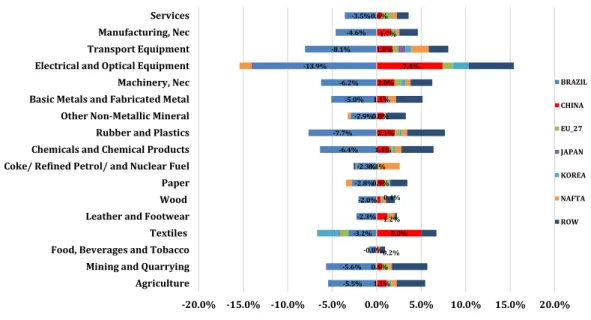
Accordingly, the share of imported intermediates over total intermediates consump-tion has risen for all sectors in the period, particularly in higher technological sectors such as Chemicals, Machinery, Transport equipment, Electrical/optical equipment and Rubber/Plastics. Figure 7shows the relative dynamics of local consumption for each country-source of intermediates by sector in Brazil, suggesting that the increase in imported intermediates was made at the expense of local intermediates for all sectors. Furthermore, among the three regions, China was by far the economy that has benefited the most over the period, increasing its relative supply of intermediates to all sectors in Brazil, including high technological sectors such as Electrical/optical equipment, Transport equipment and machinery, as well as lower-skilled labor intensive sectors such as Textiles.
-5.5% -5.6%
-0.8% -3.2%
-2.3% -2.0% -2.8%
-2.3% -6.4% -7.7%
-2.9% -5.0% -6.2% -13.9%
-8.1% -4.6%
-3.5%
1.1% 0.6% 0.2%
5.0% 1.2% 0.4% 0.9% 0.1%
1.4% 2.1% 0.8% 1.1% 2.0%
7.4% 1.8%
1.7% 0.6%
-20.0% -15.0% -10.0% -5.0% 0.0% 5.0% 10.0% 15.0% 20.0% Agriculture
Mining and Quarrying Food, Beverages and Tobacco Textiles Leather and Footwear Wood Paper Coke/ Refined Petrol/ and Nuclear Fuel Chemicals and Chemical Products Rubber and Plastics Other Non-Metallic Mineral Basic Metals and Fabricated Metal Machinery, Nec Electrical and Optical Equipment Transport Equipment Manufacturing, Nec Services
BRAZIL
CHINA
EU_27
JAPAN
KOREA
NAFTA
ROW
Source:Author’s calculation based on World Input-Output Database.
Figure 7.Evolution as a source of intermediates by sector in Brazil (1995 to 2011).
4. Estimating the Ad valorem equivalents of TBT/SPS measures
This section explains in detail the gravity specification used to estimate the ad-valorem equivalents of TBT/SPS measures on bilateral trade flows between Brazil and China, to be used as inputs in our CGE simulations (section 6).
4.1 The Gravity Equation
The gravity specification used to estimate the impacts of TBT/SPS measures on bilateral trade flows is described by this equation:
𝑦𝑖𝑗𝑠𝑡= 𝛾𝑠𝜏𝑖𝑠𝑡+ 𝛼𝑠NTB𝑖𝑠𝑡+ 𝛼𝑝𝑠NTB𝑖𝑠𝑡+ 𝑋𝑖𝑗𝑠𝑡𝜃 + 𝛼𝑖+ 𝜓𝑗+ 𝜐𝑠+ 𝜂𝑡+ 𝜀𝑖𝑗𝑠𝑡, (1) where𝑖denote the importer country (China, and Mercosur countries: Brazil, Argentina, Uruguay, Paraguay);9𝑗for the exporter country;𝑠for sector; and𝑡for the time period.
Therefore,𝑦𝑖𝑗𝑠𝑡denotes log of the (CIF) value of country𝑖’s imports from country𝑗, in sector𝑠and time period𝑡. Dummy variables𝛼𝑖,𝜓𝑗,𝜐𝑠and𝜂𝑡control for the fixed effects of importers, exporters, sectors and time, respectively. The vector𝑋𝑖𝑗𝑠𝑡represents standard gravity control variables, such as: log of GDP (both for importer and exporter), bilateral distance, common language, border sharing and colonization. We also control for relation (𝑝) and sector-relation (𝑠, 𝑝) specific dummies.10 The dummy variableNTB
𝑖𝑠𝑡controls for
sector-specific TBT/SPS measures imposed by importer𝑖in sector𝑠, which is still active in year𝑡. It is defined as a dummy variable which is equal to 1 if there exists at least one measure for that sector adopted by the importer and zero otherwise. We consider that once a measure is imposed by importer𝑖in year𝑡it also holds for the subsequent years. Moreover,𝜏𝑖𝑠𝑡denote the tariff applied by the importer𝑖in sector𝑠at year𝑡.
We are interested in estimating the effects of TBT/SPS measures within each sector for each possible bilateral combination of trade flows among Mercosur countries and China. The average effect of an TBT/SPS measure in sector𝑠is given by the coefficients𝛼𝑠and the additional effect in those sectors for a given bilateral trade relation is given by𝛼𝑝𝑠. Therefore, elasticity of imports with regard to the adoption of a regulatory measure on each sector, for each relation analyzed, are given byexp𝛼𝑠+ 𝛼𝑝𝑠− 1.11
4.2 Heckman selection model
The issue of sample selection bias in gravity models can be properly addressed through the Heckman’s selection model (Heckman,1979). In this work, we use Heckman’s model in its two-stage version. The first stage specifies a Probit model which estimates the impact of a TBT/SPS measure on the probability of a firm to become an exporter. We follow the specification described byHelpman et al.(2008) where the extensive margin decision of an exporting firm is represented by the following Probit model:
𝜌𝑖𝑗𝑠𝑡≡ 𝑃𝑇𝑖𝑗𝑠𝑡 = 1 | 𝑋= Φ𝜑𝑠𝜏𝑖𝑠𝑡+ 𝛽𝑠NTB𝑖𝑠𝑡+ 𝛽𝑝𝑠NTB𝑖𝑠𝑡+ 𝑍𝑖𝑗𝑠𝑡𝜅 + 𝑊𝑖𝑗𝑠𝑡𝜃, (2) where𝑇𝑖𝑗𝑠𝑡is an indicator variable which is equal to one if there are positive imports of country𝑖from country𝑗in sector𝑠at year𝑡;𝑍𝑖𝑗𝑠𝑡is a vector that includes all covariates (including the fixed effect dummies) from the gravity equation; and𝑊𝑖𝑗𝑠𝑡is the vector of the excluded variables that allow the identification of the selection effect. We considereda prioriseveral specifications, including the number of documents, time and cost required to export and import.
According to the work byHelpman et al.(2008) if the probability to become an exporter is somehow correlated to the decision on how much to export, the estimated impact of TBT/SPS measures on trade flows—using standard gravity OLS approaches—are likely to be downward biased. Regarding firm heterogeneity, the authors point out that standard gravity equations “confound the effects of trade barriers on firm-level trade with their effects on the proportion of exporting firms”. Accordingly, if firm heterogeneity is not somehow included as an explanatory variable in the standard gravity equation, its absence may induce an upward bias on the estimated effects of NTBs on trade flows.
10Those dummies are included in the vector𝑋
𝑖𝑗𝑠𝑡for notational convenience.
Based on the extensive margin estimation we can compute
̂ℎ
𝑖𝑗𝑠𝑡= Φ−1 ̂𝜌𝑖𝑗𝑠𝑡 and ̂𝜆𝑖𝑗𝑠𝑡≡ 𝜆 ̂ℎ𝑖𝑗𝑠𝑡=
𝜙 ̂ℎ𝑖𝑗𝑠𝑡
Φ ̂ℎ𝑖𝑗𝑠𝑡,
which are respectively aproxy for firm heterogeneity and the inverse Mills ratio (non-selection hazard). Therefore, in the second stage the inverse Mills ratio is an additional explanatory variable in the standard gravity equation such as
𝑦𝑖𝑗𝑠𝑡 = 𝛾∗𝑠𝜏𝑖𝑗𝑠𝑡+ 𝛼∗𝑠NTB𝑖𝑠𝑡+ 𝛼𝑝𝑠∗NTB𝑖𝑠𝑡+ 𝛽𝜆 ̂𝜆𝑖𝑗𝑠𝑡+ 𝑋𝑖𝑗𝑠𝑡𝛽∗+ 𝛼∗𝑖 + 𝜓𝑗∗
+ 𝜐∗𝑠 + 𝜂∗𝑡 + 𝜀∗𝑖𝑗𝑠𝑡. (3)
Equation (3) estimates the impact of a TBT/SPS measure on bilateral trade flows, conditional on the fact that firms are exporters. We also consider the specification that includes firm heterogeneity as a covariate. Based onHelpman et al.(2008), it is possible to show that the fraction of exporting firms in each exporting sector and bilateral trade flow can be estimated by ̂ℎ𝑖𝑗𝑠𝑡.12
From equation (3) we can compute the tariff equivalents of TBT/SPS measures for each GTAP sector. It can be calculated as the ratio of the sectoral elasticity of bilateral imports w.r.t. the dummy (NTB variable) over the elasticity of the same bilateral imports w.r.t. import tariffs. In the OLS model this is simply the ratio
TE𝑠𝑝= exp𝛼𝑠+ 𝛼 𝑝 𝑠− 1
𝛾𝑠 ,
for each sector𝑠and bilateral relation𝑝.13 However, for the Heckman selection model, the
tariff equivalent is calculated as the ratio of the marginal effect of the NTB over the marginal effect of the import tariff, conditional that goods are already imported (or exported). Formally, it is provided by:
𝑇𝐸𝑠𝑝 =ME(NTB𝑖𝑠𝑡)
ME𝜏𝑖𝑗𝑠𝑡
=𝔼𝑦𝑖𝑗𝑠𝑡|NTB𝑖𝑠𝑡= 1, 𝑇𝑖𝑗𝑠𝑡= 1−𝔼𝑦𝑖𝑗𝑠𝑡 |NTB𝑖𝑠𝑡= 0, 𝑇𝑖𝑗𝑠𝑡= 1 𝜕𝔼𝑦𝑖𝑗𝑠𝑡| 𝑇𝑖𝑗𝑠𝑡= 1/𝜕𝜏𝑖𝑗𝑠𝑡 ,
(4)
whereME(⋅)denotes the marginal effect computed using rather standard derivations. As illustrated, the tariff equivalent is calculated only for the group of firms that are already importers, which is consistent with the perfect competition CGE model we use in the second stage (that only accommodates the intensive margin of trade). In this regard, the
12The exact correction in order to control for firm heterogeneity is to estimate a non-linear regression including the variablelog𝛽ℎexp ̂ℎ𝑖𝑗𝑠𝑡+ ̂𝜆𝑖𝑗𝑠𝑡− 1. However, followingHelpman et al.(2008) we add ̂ℎ𝑖𝑗𝑠𝑡in a standard
linear regression. In their work, the authors show that both specifications led to the same results, although the non-linear specification is the one that is theoretically consistent with the Melitz model.
general equilibrium effects of NTBs such as TBT/SPS measures can be estimated through the calculation of their ad valorem equivalents and then through their implementation in CGE models (Gasiorek, Smith & Venables,1992;Harrison, Rutherford & Tarr,1994;
Andriamananjara et al., 2004; Andriamananjara, Ferrantino & Tsigas, 2003; Francois,
Van Meijl & Van Tongeren,2005). However, as signaled inBaldwin(2000), the notifications
of TBTs and SPSs by importing countries are likely to generate extra fixed as well as variable costs for exporting firms. Therefore, when working in conjunction with those notifications, CGE models should somehow accommodate an imperfect competition market structure able to represent export-specific fixed costs due to the existence of NTBs.14
This article uses the GTAP model on its dynamic version under a perfect competition market structure (Ianchovichina & Walmsley,2012). Therefore, in order to assure con-sistence with perfect competition, calculated ad valorem equivalents of TBTs and SPSs must represent estimations of pure extra variable costs and shall not be influenced by any kind of fixed costs. The Heckman selection model seems to be suitable for this task as long as fixed costs are not expected to exert any sort of influence on its second stage gravity equation. This must be true since fixed costs must only influence entrepreneur’s decision to become an exporter (Heckman’s first stage equation representing the effects of NTBs on the extensive margin of trade) but not his decision on how much to export, given that he is already an exporter (Heckman’s second stage equation representing the effects of NTBs on the intensive margin of trade).
5. Database and Empirical Results
Bilateral flows of imports (in current dollars) as well as import tariffs were obtained from the World Integrated Trade Solutions (WITS) of the World Bank. The data are annual from 2006 to 2013, according to GTAP sector aggregation. Tariff data used in this work are sectoral simple averages. The advantage of using simple averages—rather than the weighted averages by trade flows—is to circumvent possible endogeneity in the estimation procedure. GDP data were obtained from the World Bank. The work uses GDP data in current dollars since the HS code data were only available in current dollars as well. Additional control variables, such as bilateral distance, common language and border sharing as well as colonization were obtained from the CEPII. The number of documents necessary to import was used as the excluded variable (instrument) in the first stage of the Heckman selection model. This variable was sourced from the site “Trading across borders” of the Doing Business (World Bank).
Most of the TBT and SPS measures imposed by Mercosur countries and China were sourced from the site of the World Trade Organization (WTO). However, a significant amount of notifications reported to the WTO does not necessarily report the product codes affected by such notifications. Therefore, the database used in this work had to be complemented by additional information available from other sources such as the Brazilian National Institute of Metrology, Quality and Technology (Inmetro) and the Centre for WTO Studies (CWS). While Inmetro provided us product codes for additional TBT notifications, the CWS provided the codes for the additional SPS notifications. Product codes were available at the four-digit classification of the Harmonized System (HS04).
Last, we used a correspondence between the GTAP sectoral classification and its breakdowns at the HS04 level, assigning the GTAP sectoral classification to bilateral trade flows in the Heckman selection model.
The sample we use has 83,635 observations on positive bilateral trade flows with Mercosur countries (Brazil, Argentina, Paraguay and Uruguay) and China as the sole importers over the period 2006–2013. When zero trade flows are added to the sample, the number of observations rises to 323,015. Over the years, nearly 74% of the observations corresponded to zero trade flows, suggesting a high potential for sample selection bias when only positive trade flows are considered in standard gravity estimations.
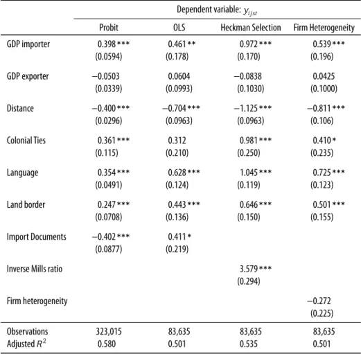
The third column inTable 2reports standard (pooled) OLS estimates of a gravity model. The estimated coefficients have the expected signs and are mostly significant at the 1% level, exception made for the estimates on the impact of the exporting country’s GDP, which is not statistically different from zero. The second column reports the estimations of a Probit model with basically the same set of explanatory variables as the model in column three and corresponds to the first stage of the Heckman selection model. The Probit model estimates the impacts of traditional gravity variables on the probability to become an exporter. The significance of the estimated coefficients suggests a likely correlation between the decisions on how much to export (import) and the probability to become and exporter. This is the second piece of evidence on the existence of sample selection bias in traditional OLS gravity estimates. For identification reasons related to the second stage estimations of the Heckman selection model, we considered several measures related to costs of importing and exporting, such as time, cost and number of documents required for both. In our estimations, the number of documents required to import was the only variable that was statistically significant in the Probit model but not in the second stage OLS model. Therefore, it was used as the excluded variable, i.e., introduced in the first stage but not in the second stage of the Heckman selection model.15
According toMelitz(2003), the sectoral extensive margin of trade is determined by the heterogeneity on the productivities of domestic firms. In other words, the more productive firms will become exporters and the less productive ones will only sell domestically. A zero-profit condition determines endogenously the productivity threshold. Accordingly, sectors facing higher fixed costs to export are likely to sell lower volumes abroad, since only a few most productive firms might be able to retain positive profits from the exporting activity. As long as “the number of documents to import” in the destination country constitutes an additional fixed cost of exporting firms in source countries, it should exert a negative and statistically significant effect on the probability of a firm to become an exporter, as it is shown in the second column ofTable 2. As a fixed cost, however, it should have no influence on the marginal decision on how much to export, given that a firm is already exporting, as it seems to be the case according to estimations reported in the third column.16
The Mills ratio estimated in the first stage (second column) is then used as an additional explanatory variable in the second stage (fourth column) of the Heckman selection model. Estimations reported in column four reveal two important facts. First, the high significance of the Mills ratio corroborates the existence of sample selection bias and the importance
15We only present the final specification of the excluded variable to save space.
Table 2.Two-stage Heckman selection model (2006–2013).
Dependent variable:𝑦𝑖𝑗𝑠𝑡
Probit OLS Heckman Selection Firm Heterogeneity GDP importer 0.398∗∗∗ 0.461∗∗ 0.972∗∗∗ 0.539∗∗∗
(0.0594) (0.178) (0.170) (0.196)
GDP exporter −0.0503 0.0604 −0.0838 0.0425 (0.0339) (0.0993) (0.1030) (0.1000) Distance −0.400∗∗∗ −0.704∗∗∗ −1.125∗∗∗ −0.811∗∗∗
(0.0296) (0.0963) (0.0963) (0.106) Colonial Ties 0.361∗∗∗ 0.312 0.981∗∗∗ 0.410∗
(0.115) (0.210) (0.250) (0.235)
Language 0.354∗∗∗ 0.628∗∗∗ 1.045∗∗∗ 0.725∗∗∗ (0.0491) (0.124) (0.119) (0.123) Land border 0.247∗∗∗ 0.443∗∗∗ 0.646∗∗∗ 0.501∗∗∗
(0.0708) (0.136) (0.150) (0.155)
Import Documents −0.402∗∗∗ 0.411∗ (0.0877) (0.219)
Inverse Mills ratio 3.579∗∗∗
(0.294)
Firm heterogeneity −0.272
(0.225) Observations 323,015 83,635 83,635 83,635
Adjusted𝑅2 0.580 0.501 0.535 0.501
Notes:The simulations in each column also control for the interactions between an existing measure (dummy variable) and each of the 42 GTAP sectors (sectoral dummy variables). All regressions include sectoral, importer, exporter and time dummies. Sector clustered standard errors in parenthesis (corrected for two-step procedure for Heckman and Firm heterogeneity models).∗Significant at 10%;∗∗Significant at 5%;∗∗∗Significant at 1%.
of taking zero trade flows into account when working with gravity models. Second, not controlling for the existence of sample selection bias in traditional gravity estimations may lead to downward biased estimates.
In the last column ofTable 2theproxyvariable for firm heterogeneity is then added to the second stage gravity equation. Results suggest that its impact is not statistically different from zero. The insignificance of firm heterogeneity may be explained, at least in part, due to a low number of exporting firms in Brazil, where only a few multinationals firms with higher than average productivity levels are responsible for most of the exports in the country.17
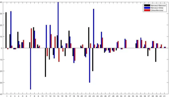
Results reported inFigure 8shows the sectoral impacts of existing measures (TBT/SPS) on bilateral trade flows among Mercosur countries, on Mercosur countries’ bilateral imports
Source:Author’s calculation based on the Probit model (First stage for Heckman model). See text for details.
Figure 8.Sectoral impacts of NTBs on the probability to become an exporter (%).
from China and on China’s imports from Mercosur countries, respectively, for each one of the 42 GTAP sectors.
All the estimations were derived from the first stage Probit model and therefore measure the likely impacts of existing notifications on the probability of a firm to become an exporter at each GTAP merchandise sector level, in each source country (i.e. Mercosur countries and China).
According toFigure 8, the imposition of an NTB by an importing country may have contrasting sectoral effects on the exporting country. For instance, when a typical country from Mercosur imports from China, pre-existing TBT/SPS in GTAP sector 7 decreases the sectorial probability of a Chinese firm to become an exporter to Mercosur by over 30%. In contrast, the imposition of non-tariff barriers in GTAP sector 23 increases the sectorial probability of a Chinese firm to become an exporter to countries in Mercosur by more than 30%. These two apparently conflicting results may be reconciled when a more careful look is given to the expected firm-level effects of a TBT/SPS. Accordingly, the imposition of a given measure by an importing country may exert simultaneous and conflicting effects on the exporting firm’s demand, marginal costs and fixed costs. This is the reason behind the apparent ambiguity when the net effects of measures on firm’s behavior are evaluated. For instance, when the fixed cost effect of a measure is dominant, it will affect negatively the extensive margin of trade, meaning that the probability of a firm to become an exporter will decrease. On the other hand, when the demand effect of a given measure is dominant18,
it will increase the probability of a firm to become an exporter. It is worth noting that when it comes to the intensive margin of trade (second stage equation), variations in fixed effects
due to the imposition of a given measure play no role in the decision of a firm on how much to export.
Results inTable 3show the estimated tariff equivalents of existing TBT/SPS for each GTAP sectorial trade flow among countries in Mercosur and China. These tariff equivalents are calculated from the marginal effects of sectoral measures and tariffs on bilateral imports estimated from the second stage equation of the Heckman selection model. For the non-reported tariff equivalents in the Table, it means that its calculated impacts on bilateral trade flows were either positive or not statistically different from zero.
In general, results inTable 3suggest that the protectionist effects of existing TBT/SPS are more relevant for bilateral imports among Mercosur countries and for Mercosur’s imports from China (column 3) than for China’s bilateral imports from Mercosur countries (column 4). While the negative effects of existing TBT/SPS on Mercosur’s imports from China seem to be evenly spread among sectors, the same effects from the perspective of Chinese imports from Mercosur seem to be concentrated in the Agribusiness sector. Due to its very nature, this is a sector with a higher incidence of SPS than TBT.
Moreover, due to the asymmetric distribution of tariff equivalents among sectors in
Table 3, any uniform reduction of pre-existing NTBs for bilateral trade flows among
Mercosur countries and China, resulting from a hypothetical PTA, would be probably more beneficial for China’s exports to Mercosur than the other way around.
6. Case Study
This section presents the main economic impacts of a hypothetical free trade agreement between Mercosur and China on the economy of Brazil. The analysis in this section goes beyond the traditional CGE impact analysis based on gross trade flows and proposes a more precise representation of the likely impacts of PTAs in a globally fragmented economy, where trade in intermediates represent more than 66% of global trade in goods and services. This value-added approach connects the traditional CGE analysis of PTAs with an auxiliary input-output model that is able to convert gross results into valued-added figures. Our methodology is also related to the empirical works of bothJohnson & Noguera(2012b) and
Koopman et al.(2014), and allows comparisons of value added exported as well as the share
of reprocessing of imported intermediates over total imports at pre and post simulation equilibriums.
6.1 CGE model and database
Our general equilibrium exercise uses the extended GTAP 9 database for dynamic re-cursive models.19 This database combines detailed information on bilateral trade flows,
transportation and trade protection, representing trade relations among 140 regions and 57 sectors/region, together with national input-output tables for each region as well as information on interregional income flows. The database is then harmonized and completed with additional information from the World Bank and IMF, resulting in a rather realistic description of the world economy for 2011 (the last version of the GTAP database). The database was then updated till 2016 using real data for GDP, labor force and population for each region, sourced from both World Bank and CEPII (Centre d’Etudes Prospectives
Table 3.Ad valorem equivalents (%) of NTBs by GTAP sector and bilateral relation.
Sectors Mercosur-Mercosur Mercosur-China China-Mercosur Extractive
Fishing 0.71 – –
Coal – – –
Oil 1.45 1.2 0.29
Gas 1.46 – –
Agribusiness
Bovine meat products 20.87 17.71 17.71 Vegetables, Oils and fats 10.18 – – Dairy products 17.9 18.9 19.18
Processed rice – 19.57 18.23
Sugar 20.56 – 9.36
Food prod. nec. 9.58 8.87 4.68
Beverage/Tobacco – 4.96 5.39
Manufacturing
Textiles – 8.29 –
Wearing apparel – 9.95 1.69
Leather products – 8.92 –
Wood products 3.63 7.8 –
Paper products 6.28 – –
Petroleum/coal prod. – 7.25 –
Mineral products nec 3.39 – –
Metals nec – 8.35 –
Metal products 1.93 – –
Motor vehicles/parts – 11.41 2.27
Transport equipment – 9.46 –
Electronic equipment – – 0.86
Manufactures nec. 4.96 – –
Source:Author’s calculation based on the OLS model (Second stage of Heckman’s model). See text for details.
et d’Informations Internationales). The baseline trajectory for impact analysis was then projected from 2016 till 2030, using the same set of (forecasted) variables.
The GDyn model (Ianchovichina & Walmsley,2012) was used in order to evaluate the long run effects of a PTA between Mercosur and China on the economy of Brazil. GDyn is a large-scale recursively dynamic AGE model representing the global economy. The model identifies 57 sectors in each of 140 regions of the world. Its system of equations is fully based on microeconomic foundations providing a detailed specification of household and perfect competitive firm behavior within individual regions and trade linkages between regions, according to the standard Armington hypothesis (Armington,1969) in large scale CGE models. The model extends the static version of GTAP model (Hertel,1996) to include international capital mobility, capital accumulation, and an adaptive expectations theory for investment.
allows the analysis of policy shocks that affect economic incentives to invest overseas, such as the ones related to the outsourcing of production. In this sense, the GDyn model seems particularly suitable for the purpose of evaluating the likely effects of PTAs on the formation of GVCs as long as foreign capital ownership can be taken into account and GVC income flows can be better traced out.
The GDyn model also classifies as a Johansen type model (Dixon & Jorgenson,2013)20
in the sense that it estimates the general equilibrium effects of external shocks using comparative statics analysis, period by period. In this regard, the model solves a system of linearized equations, comparing two different equilibrium states, after each periodic (usually one year) process of adjustment (if any). Results for a given endogenous variable (like GDP, volume exported/imported, etc.) is reported according to percentage differences between their estimated values in two distinct trajectories (baseline and policy) over the period 2017–2030. On one hand, the “baseline” trajectory reports the world economy as if the policy shocks under evaluation had not taken place, using forecasts for countries’ GDP, labor force and population as model inputs. On the other hand, the “policy” trajectory reports the world economy when the same policy shocks are allowed to take effect, according to a fully endogenized model dynamics.
Model closure considers perfect inter-sectorial mobility of production factors such as labor and capital and imperfect mobility for land and natural resources. Returns of investments are equalized among regions and firms’ technology is exogenous. Non-tariff barriers are modelled as “iceberg” transport costs, followingHertel et al.(2001)
6.2 Simulation results
6.2.1 The big picture: standard macro results
Table 4shows the simulated impacts of a comprehensive FTA involving Mercosur countries
and China in two distinct scenarios. First, we consider a PTA between Brazil and China and then another PTA where Mercosur countries negotiate as a block. In both scenarios we assume full elimination of bilateral import tariffs as well as a 50% reduction in bilateral TBT/SPS barriers (according tosection 5). By 2030, additional GDP growth in Brazil is expected to reach 0.56% per year, reflecting additional investments of 2.50% per year and greater participation in global trade. When Brazil is the sole country to negotiate, the rest of
Table 4.Macroeconomic Effects of a FTA between Mercosur and China (in %, 2030).
FTA: Only Brazil and China FTA: Mercosur and China
GDP Exports Imports Investment GDP Exports Imports Investment
Brazil 0.56 5.4 6.86 2.5 0.56 5.47 7.01 2.5
Argentina −0.07 −0.24 −0.18 −0.04 1.04 4.19 6.63 3.46
Venezuela 0.02 0 0.2 0.13 0.49 3.72 5.76 1.24
Paraguay −0.16 −0.13 −0.3 −0.45 0.53 3.64 3.29 1.89 Uruguay −0.13 −0.16 −0.3 −0.27 3.23 7.11 11.17 8.68
China 0.09 0.24 0.47 0.21 0.15 0.39 0.76 0.36
Source:Author’s calculation based on GDyn model.
20Johansen solutions are currently standard in the CGE literature (seePearson, Parmenter, Powell, Wilcoxen &
Mercosur are expected to be worse off with the agreement (column 2). This is an expected result, as these countries lose market-share in Brazil due to cheaper competing imports from China. Given the much larger size of China’s economy, long term trade gains in this economy are expected to be less impressive in comparison to the ones obtained by Brazil. When Mercosur countries negotiate as a block (columns 6 to 9), the long-term results for Brazil remain basically unchanged, reflecting its larger size and the fact that bilateral tariffs among Mercosur countries are currently quite close to zero. In this scenario, the rest of Mercosur is clearly better off. In the case of Argentina, the second largest economy in Mercosur, additional GDP gains per year are expected to reach 1.04% by 2030. China is expected to be slightly better off in this second scenario, with additional GDP gains of nearly 0.15% per year in the long term.
6.2.2 Export and import flows: standard and value-added approaches
Table 4reported general macro results in standard CGE analysis. Since nowadays nearly
70% of global exports correspond to trade in parts and components, it seems important to report and compare long-term growth in gross trade flows as well as in value added exported.
Table 5reports the long-term impacts on Brazil’s bilateral exports of a comprehensive
PTA involving Mercosur and China. By 2030, the economy of Brazil is expected to increase it’s per year gross exports to its main trade partners (China, USA and EU), with the exception of Argentina, where the Brazilian economy is expected to be exporting less to (−8.15%, per year), as a consequence of the agreement. However, when the growth in value added generated by exports is taken into consideration, figures are generally lower, suggesting that standard CGE analysis focused on gross trade figures may overestimate trade income gains generate by the agreement. In particular, while Brazil’s gross exports to Uruguay is expected to be 11% higher by 2030, domestic value added per year generated by these exports is expected to decrease by −3.69%. In the case of Argentina, the loss in domestic value added is greater than the loss in gross exports.
The positive difference between the increase in gross exports and value added exported reported inTable 5is a clear sign that the foreign content embedded in Brazil’s exports has increased as a consequence of the agreement, reflecting a higher prevalence of trade in intermediates among Brazil and some of its main trade partners, such as USA, EU, China
Table 5.Impacts on Brazilian exports and imports by partner (in %, 2030).
Exports Inports
Destination Gross Value-added Difference Gross Value-added Difference
USA 3.46 3.14 0.32 −13.46 −12.08 −1.38
EU 2.62 2.51 0.11 −11.46 −9.73 −1.73
Argentina −8.15 −10.17 2.02 −0.8 −1.85 1.05
China 7.69 7.51 0.18 69.02 57.61 11.41
Row 2.95 2.78 0.17 −7.26 −0.83 −6.43
Venezuela 55.23 52.54 2.69 4.57 3.15 1.42 Paraguay −6.9 −8.59 1.69 2.17 1.19 0.98 Uruguay 11.02 −3.69 14.71 −3.25 −3.55 0.3
Total 4.56 4.07 0.49 5.34 4.85 0.49
and Argentina, despite the prediction of lower export volumes to its main trade partner in Mercosur. The higher foreign content embedded in Brazil’s export is expected to improve the competitiveness of its goods abroad, increasing its penetration in larger and more competitive markets in the USA, EU and the rest of the world.
When it comes to bilateral imports, the difference between gross import flows and value added imported by the Brazilian economy is positive for all countries involved in the FTA. This is also suggestive of a greater prevalence of trade in intermediates among countries in Mercosur and China, probably reflecting a higher foreign content embedded in goods and services imported by the Brazilian economy from its PTA partners. Results inTable 5
are also suggestive that the significant increase in Brazilian imports from China is made at the expense of imports from the USA and EU. To the extent that imports from China may replace more efficient suppliers in those regions, this may result in trade diversion, partially reducing potential welfare gains in Brazil.
6.2.3 Bilateral trade flows at the sector level: standard and value-added approaches
Results inTable 6report the likely impacts of the Mercosur–China FTA on bilateral trade between Brazil and China at several GTAP sector levels. As suggested by the numbers reported in the Tables, differences between gross trade and trade in value added are even more impressive when comparisons are made at a more disaggregated sectoral level.
In particular, “mercantilist” type analyses focused on gross trade imbalances may prove to be misguided when it comes to the sectoral evaluation of net income generated by exports. Again, the differences reported inTable 6may reflect a higher prominence of
Table 6.Impact on Brazil’s bilateral trade with China (in %, 2030).
Exports Inports
Sectors Gross Value-added Difference Gross Value-added Difference Agriculture
Paddy rice 8.9 21.1 −12.1 32.1 67.4 −35.3
Wheat 4.7 32.1 −27.4 −5.5 72.3 −77.8
Cereal grains nec 3.4 31.6 −28.2 11.6 64.3 −52.7 Vegetables, fruit, nuts 61.7 29.9 31.8 55.5 63.1 −7.7
Oil seeds 4.5 4.9 −0.43 52.3 50.9 1.4
Sugar cane, sugar beet – 14.3 −14.3 −1.7 56 −57.6 Plant-based fibers 15.2 11.4 3.8 5.3 83.2 −77.9
Crops nec 45 37.5 7.5 67.8 49.8 18
Bovine cattle, sheep, goats, horses 17.7 33.2 −15.5 14.6 74.8 −60.2 Animal products nec 53 41.2 11.7 19.5 76.3 −56.8 Wool, silk-worm cocoons 49.4 1,531.5 −1,482.1 4.4 80.7 −76.2 Extractive
Forestry 20.5 11 9.5 35.2 54.7 −19.4
Fishing −0.3 27.2 −27.5 14.9 55.5 −40.6
Coal 36.9 8.4 28.5 −0.6 42.8 −43.4
Oil −0.3 2.5 −2.8 6.5 34.8 −28.3
Gas – 5.5 −5.5 – 46.1 −46.1
Minerals nec 0.5 1.2 −0.6 5 60.2 −55.2
trade in intermediates involving Brazil and China as well as third countries, with likely consequences to the way goods and services are produced in both regions.
For instance, results for Brazilian agricultural sectors inTable 6suggest that annual growth in sectoral value added generated by exports are expected to be systematically higher when compared to gross export growth by 2030. Therefore, gross trade figures reported for those sectors may now quite well underestimate the expected sectoral net income growth due to the agreement. This is mainly the consequence of three effects that reflects the very nature of trade in agricultural goods. First, the foreign content embedded in natural resource intensive goods such as agriculture is usually low. Second, agricultural intermediates may also be indirectly exported to China embedded in other sectors’ exports of final goods in Brazil. Third, Brazil’s exports of agricultural intermediates to other countries may be later reprocessed and redirected to China, following the logic of GVC. The last two kinds of indirect exports do not show up as gross exports to China in standard national input-output tables. The same is obviously true from the point of view of Brazilian imports and may help to explain why Brazil’s imported value added in agricultural goods is systematically higher than gross imports.
When it comes to bilateral trade in both agribusiness and manufacturing, results in sug-gest a different trade logic in comparison to the one described above. First, the production and exporting of manufactures are, in general, not constrained by the existence of domestic natural resources. This helps to explain the ongoing predominance of international supply chains in manufacturing sectors and the higher foreign content embedded in the exports of manufactured goods in comparison to other goods such as agricultures (backward linkages). Second, manufactured intermediates are usually inputs for the production of final goods in other manufacturing sectors, which weakens the creation of value added through indirect (domestic) exports. Last, indirect exports through third countries are clearly a possibility for the exports of manufactured goods (forward linkages). Therefore, in more complex sectors such as agribusiness and manufacturing, Brazilian gross exports would be expected to grow faster than the domestic value added they create. This is precisely the result reported
inTable 7, a clear sign that Brazil’s manufactured exports to China are expected to carry a
higher foreign content of intermediates in the long term as a consequence of the agreement. Regarding Brazil’s imports of manufactured goods from China, gross imports are expected to grow faster than value added imported by 2030, suggesting that China’s manufac-tured exports to Brazil are also expected to employ a higher foreign content of intermediates in the long term.
Results are therefore suggestive that long-term changes in relative prices are expected to be associated with structural changes when it comes to bilateral trade between Brazil and China. This issue will deserve a more comprehensive and detailed analysis in the following section.
6.2.4 Connecting to Global Value Chains: Are there signs of integration?
Results inTable 8show the macro sectorial “vax ratio”21for exporting sectors in Brazil. It
turns out that the qualitative behavior is basically the same as the one described for sectoral bilateral trade between Brazil and China. While Brazil is expected to add a greater share of foreign inputs within its total exports of manufactured (including agribusiness) and service
Table 7.Impact on Brazil’s bilateral trade with China (in %, 2030).
Exports Inports
Sectors Gross Value-added Difference Gross Value-added Difference Agribusiness
Bovine meat products 358.3 35.6 322.7 107.6 103.4 4.2 Meat products nec 52 42.3 9.6 223.9 103.2 120.7 Vegetable oils and fats 3.3 5.2 −1.9 69.3 52.9 16.4 Dairy products 331.8 20.2 311.5 276.5 91.7 184.8
Processed rice 50.6 12.6 38 170.2 61.1 109.1
Sugar 25.1 11.4 13.8 88.4 53.8 34.6
Food products nec 68.3 32.9 35.4 51.7 57.9 −6.2 Beverages and tobacco products 96.6 11.9 84.6 36.4 57.4 −21.1 Manufacturing
Textiles 121.9 8.1 113.7 99.3 82.5 16.7
Wearing apparel 238.7 30.7 208 125.2 98.9 26.3 Leather products 76.5 70.1 6.4 178.7 137.9 40.7
Wood products 9 8.4 0.6 142.7 62.9 79.8
Paper products, publishing 7.8 7.9 −0.1 81.1 57 24.2 Petroleum, coal products 34.3 6.7 27.6 11.1 34.9 −23.8 Chemical, rubber, plastics 68.6 13.3 55.2 45.7 48 −2.3 Mineral products nec 106.4 11.3 95.1 60.2 52.6 7.6
Ferrous metals 25.4 13.7 11.7 52.8 63.8 −11
Metals nec 53.7 15.8 38 115.4 65.2 50.1
Metal products 122.2 7.2 115.1 107 68.5 38.5
Motor vehicles and parts 81.4 33 48.4 171 95 76 Transport equipment nec 50.5 23.3 27.2 226.2 162.3 63.9 Electronic equipment 37.9 5.6 32.4 49.2 42.2 7 Machinery and equip. nec 102.9 21.3 81.5 87.4 72.2 15.2 Manufactures nec 252.1 13.9 238.2 75.9 65.2 10.6
Services 81 11.8 69.2 −2.3 49.9 −52.3
Source:Author’s calculation based on GDyn model.
Table 8.Sectoral Vax Ratio.
Sector Baseline Policy Impact (%) Agriculture 0.999 1.01 1.12 Extractive 0.794 0.803 1.12 Manufacture 0.489 0.482 −1.56 Services 3.165 3.086 −2.49
Source:Author’s calculation based on GDyn model.