BAR, Rio de Janeiro, v. 15, n. 1, art. 3, e170072, 2018
http://dx.doi.org/10.1590/1807-7692bar2018170072
Sponsor Bias in Pension Fund Administrative Expenses: The
Brazilian Experience
Claudio Marcio Pereira da Cunha1
Universidade Federal do Espírito Santo, Centro de Ciências Jurídicas e Econômicas, Vitória, ES, Brazil1
Abstract
Previous literature has reported that pension funds sponsored by public organizations present greater administrative expenses when compared to similar pension funds sponsored by private organizations. We investigate this sponsor bias, hypothesizing that it may originate from the omission of relevant control variables, specifically variables for location of headquarters and the level of outsourced services. We test this hypothesis by linear regression in the cross-section of 164 Brazilian closed pension funds, using annual data from 2010 to 2014. We find that these control variables partly explain the sponsor bias, especially for medium-size pension funds, and when the sponsor is an organization related to a state or municipal government. We also hypothesize that political bias may increase administrative expenses of public sponsor pension funds, especially in election years. We test this hypothesis by panel regression using a fixed effects method and did not find statistically significant changes in administrative expenses in election years. Our findings do not support the hypothesis of political bias in administrative expenses of Brazilian closed pension funds. On the contrary, we present evidence that the sponsor bias may be driven by characteristics of the pension funds omitted in previous literature.
Introduction
The importance of pension funds grows as populations age. Pension values depend directly on the net return obtained on pension fund assets. Administrative expenses deducted from gross return may play a significant role in net return. In a simulation performed by Bikker and De Dreu (2009), if annual administrative expenses increase from 1% to 2% of total fund assets, retirement income may drop around 25% (assuming 5% of annual real rate of return).
The literature concerned with pension fund administrative expenses has two main goals. One goal is to identify potential scale economies, as in Caswell (1976). If there are economies of scale, merging pension funds may be beneficial to participants. Consequently it is interesting to find out if there is an optimal pension fund size, as in Bikker (2017). The other goal related to pension fund administrative expenses is concerned with the factors that drive them, as in Bikker, Steenbeek and Torracchi (2012), that investigate the effect of plan characteristics. In this study we develop the second approach, dissecting previous findings.
In most developed countries, the institutional structure of pension systems are organized upon 3 pillars. The first pillar comprises a public pension scheme, usually mandatory, financed on a pay-as-you-go (PAYG) basis. Because it usually pays a defined benefit and may be complemented by taxes, the effect of administrative expenses to participants is limited. Most studies on administrative expenses focus on the second pillar, which comprises closed pension funds. These are collective private organizations, where participants share a professional link to the sponsor, an organization that may be public, private or professional. Closed pension funds are financed solely by contributions from participants and sponsors, implying that contributions and benefits are directly affected by fund performance, thus, by administrative expenses. The third pillar are tax-deferred individual accounts provided by financial institutions, compensated by fees, charged usually as a percentage of account balance. There is freedom to move individual accounts from one institution to another (portability). Thus, administrative expenses are less relevant, because participants do not necessarily benefit from low expenses and they can more easily avoid high expenses (Bikker, Steenbeek, & Torracchi, 2012; Bikker, 2017).
In Brazil, the basic difference from the system described above is that the public pension scheme is divided into a General Social Security System (in Portuguese, Regime Geral de Previdência Social – RGPS), for private sector workers, and a pension regime for government workers (called, in Portuguese, Regimes Próprios de Previdência Social – RPPS) (Associação Brasileira das Entidades Fechadas de Previdência Complementar [ABRAPP], 2014).
However, the focus of present study is not on public pension schemes, but on administrative expenses of Brazilian complementary sponsored closed pension funds, known by the abbreviation EFPC (Entidades Fechadas de Previdência Complementar, in Portuguese), which are private entities that correspond to the second pillar in the system described for most developed countries.
EFPC are directed at medium and high income workers to preserve their living standards after retirement, since the GSSS (or, in Portuguese, Regime Geral de Previdência Social [RGPS]) has a ceiling for the value of pensions, and has been oriented to play a distributive role. Sponsors may be state-owned companies (public sponsor), private companies (private sponsor), or labor unions and professional associations (group sponsor) (ABRAPP, 2014).
EFPC represent a large share of savings in Brazil, being responsible for a large fraction of retirees’
and beneficiaries’ incomes. By the end of 2015 the summed assets of EFPC added up to R$ 721 billion
Bikker et al. (2012), for Australia, Canada, the Netherlands, and the United States, and Abi-Ramia, Boueri and Sachsida (2015), for Brazil, have reported a sponsor bias in administrative expenses of closed pension funds. Both studies show evidence that funds with public sponsors (either state-owned companies or local governments) present greater administrative expenses, after controlling for assets, number of participants and fund characteristics. However, neither of them investigated the reason for this sponsor bias. The main objective of the present study is to investigate possible causes for the greater administrative expenses for public sponsored pension funds (sponsor bias) in Brazil.
Hypotheses
We test three hypotheses that may explain the sponsor bias. First, we hypothesize that public sponsored pension funds are located in cities with higher costs of living, which imposes higher prices to production factors, mainly labor. Indeed, almost half of public sponsored pension funds are related to the federal government, which implies that most of the employees are located either in Brasilia (the capital of Brazil), or in Rio de Janeiro (the former capital of Brazil, that still concentrates some federal activities). These metropolitan regions, along with São Paulo, historically present the greatest costs of living in Brazil (Almeida & Azzoni, 2016). We evaluate the influence of location on total administrative expenses using dummies for location.
Our second hypothesis is that public sponsored EFPC insource portfolio management activities. A way to outsource portfolio management is to allocate assets to investment funds. In this case, the cost of portfolio management may be deduced from the net return of the asset, instead of being accounted for as administrative expenses. Thus, insourcing portfolio management may imply higher administrative expenses when compared with similar pension funds that outsource this activity. There are at least three reasons for public sponsored EFPC to insource portfolio management more than other EFPC. First, public sponsored EFPC have more assets than private or group sponsored pension funds, meaning that they benefit more from insourcing activities due to the economies of scale. In 2015 there were 76 public sponsored EFPC, representing 28% of the total number, and 64% of summed assets of all EFPC (PREVIC, 2015). Second, insourcing portfolio management allows activism by pension funds in equity investment, that can improve firm valuation, as reported by Giannetti and Laeven (2009). But, again, pension funds must be large to benefit from activism, because it is necessary to own large stakes of companies to influence their administration. And third, discretionary power in portfolio allocation may also be used politically, as reported by Bradley, Pantzalis and Yuan (2016) , and public pension funds would be more exposed to political interference.
Finally, we hypothesize that public sponsors may have discretionary power over administrative expenses, directing fund resources to support political activities. In Brazil, Lazzarini, Musacchio, Bandeira-de-Mello and Marcon (2015) report that the firms that donate to winning candidates are more likely to receive funding in the form of loans from the state owned National Development Bank (Banco Nacional de Desenvolvimento Econômico e Social - BNDES). Carvalho (2014) provide evidence that BNDES may have acted to induce employment expansion in politically attractive regions immediately before competitive elections. Thus, we test if administrative expenses of public sponsored EFPC increase in electoral years, which would indicate the use of fund resources to influence elections.
Pension Funds Administrative Expenses
investment activities (portfolio management). He considers the total number of participants and total assets as adequate output proxies, respectively. However, the analysis only took the number of total participants as an output proxy, along with control variables, arguing that it would be inadequate to consider both output proxies, due to strong correlation between them.
Mitchell and Andrews (1981) generalize Caswell’s methodology. They postulate a Cobb-Douglas cost function, to consider both outputs in the same analysis, modelling administrative expenses as represented in equation (1), where AdmExp is total administrative expenses, Pop is the number of total participants, Assets is total assets, P refers to input prices, is an error term, , 1, 2, and are
parameters of the model, andi is an index that identifies pension plans.
ln(𝐴𝑑𝑚𝐸𝑥𝑝𝑖) = 𝛼 + 𝛽1ln(𝑃𝑜𝑝𝑖) + 𝛽2ln(𝐴𝑠𝑠𝑒𝑡𝑠𝑖) + 𝜑 ln(𝑃𝑖) + 𝜀𝑖 (1)
In their final model, represented in equation (2), Mitchell and Andrews (1981) add control variables (the vector X), with a corresponding vector of parameters (), and omit input prices (P), arguing that prices do not vary systematically across plans, but acknowledge that this omission would be serious in a time series study. However, if plan headquarters are placed in different locations and labor costs are significantly different between locations, a proxy for input prices should be considered. If location is correlated with any of these control variables, parameters estimates from linear regressions will probably be biased due to an omitted variable problem. This is a point we explore in the present study. Mitchell and Andrews (1981) confirm the finding of Caswell (1976) that there are significant economies of scale in the administration of private pension plans.
ln(𝐴𝑑𝑚𝐸𝑥𝑝𝑖) = 𝛼 + 𝛽1ln(𝑃𝑜𝑝𝑖) + 𝛽2ln(𝐴𝑠𝑠𝑒𝑡𝑠𝑖) + 𝜸 𝑿𝒊+ 𝜀𝑖 (2)
The model in equation (2), omitting price variables, has been pervasive in literature related to pension fund administrative expenses. Bateman and Mitchell (2004) apply a similar model to Australian pension plans, changing control variables. They find that, for defined benefit plans, reported expenses are about one-third higher than for defined contribution plans. They also find that retail plans, opened to the general public, have expenses that are 70% higher than plans with employer sponsors.
Bikker et al. (2012) also apply a model similar to that represented in equation (2), for pension funds in Australia, Canada, the Netherlands, and the United States. Besides using a different set of control variables, they perform panel data analysis, incorporating time dimension to the sample, and using annual values for variables from 2004 to 2008. Each observation is identified by three indexes: plan, country and time. They focus the analysis on closed employer sponsored funds that provide complementary income to retirees, as does the EFPC in Brazil. The focus of control variables is on service quality and complexity of pension plans. These variables are evaluated through scores based, respectively, on 12 and 15 items. As expected, they find that both service quality and complexity significantly increase administrative expenses. Both are also related to size, with smaller funds tending to provide fewer services and be less complex. Additionally, they find that funds with public sponsors present higher expenses than nonpublic sector sponsors. We refer to this difference between public and nonpublic sponsored fund as sponsor bias, which is the point that we aim to investigate deeper in the present study.
Abi-Ramia et al. (2015), as well as Bikker et al. (2012), use panel data analysis on a model similar to equation (2), but for a sample of Brazilian EFPC (closed pension funds), in years 2010 and 2011. Each observation is identified by a fund index and by a time (year) index, as expressed in equation (3), where all variables and parameters follow the same description as in equation (2). They also find, as Bikker et al. (2012), that public sponsored funds present higher expenses (sponsor bias). However, they do not investigate its causes.
ln(𝐴𝑑𝑚𝐸𝑥𝑝𝑖𝑡) = 𝛼 + 𝛽1ln(𝑃𝑜𝑝𝑖𝑡) + 𝛽2ln(𝐴𝑠𝑠𝑒𝑡𝑠𝑖𝑡) + 𝜸 𝑿𝒊𝒕+ 𝜀𝑖𝑡 (3)
and total assets in the other. They investigate the effects of governance and outsourcing on pension fund expenses. They find that funds sponsored by professional groups (which we call group sponsor) are the most expensive, which they attribute to the decentralized operational environment. They also find that, as expected, the level of outsourcing is inversely related to fund size, and raises administrative costs significantly. This supports our conjecture that larger funds, such as the EFPC in Brazil, should insource activities. However, we cannot separate expenses related to administrative activities from those related to investment activities. For this reason, when funds insource activities, they possibly internalize administrative costs related to investment activities. When investment activities are outsourced, these costs may be hidden as deductions from return on portfolio. Thus, looking at total EFPC administrative expenses, using data available in Brazil, outsourcing may underestimate expenses, due to omission of costs related to investment activities. We evaluate whether sponsor bias can be at least partly attributed to insourcing of activities by EFPC with public sponsors.
Political Bias in Public Organizations
Previously we discussed possible sources for the sponsor bias that stem from two operational characteristics: location and outsourcing. Higher administrative expenses related to these characteristics are not signs of waste of resources. Now we discuss the agency problem in pension funds management that are detrimental to fund performance. Empirical evidence indicates that pension funds, particularly public sponsored funds, present political bias in resource allocation that delivers poor returns on assets, when compared to alternative similar unbiased allocations.
Brown, Pollet and Weisbenner (2009) document that public pension funds in the United States present substantial home bias in their portfolio allocation, meaning that they overweight the holdings of stocks of companies that are headquartered in-state. They also provide evidence that this home bias is more likely in more corrupt states. Their sample contained 20 state pension plans, and they used quarterly data from the first quarter of 1980 to the third quarter of 2008. Later they expanded their sample to 27 state pension plans (Brown, Pollet, & Weisbenner, 2015), and the time span of data to 2008. They confirm previous findings and additionally provide evidence that local bias is related to election financing and outcome: it is more likely that public pension plans hold stock of firms located in states where a high fraction of their campaign contributions were directed to the current governor. However, in both studies, authors observe excess returns through in-state investments, indicating that this local bias does not hurt fund performance.
Hochberg and Rauh (2013) document local bias in private equity investment in the United States. They find it particularly pronounced for public pension funds. Conflicting with evidence provided by Brown, Pollet and Weisbenner (2015) related to common equity, Hochberg and Rauh (2013) report that public pension funds underperform in their in-state private equity investments, which present returns 2-4% points lower than both their own similar out-of-state investments and similar investments in their state by out-of-state investors. They also provide evidence that home-bias may have political roots, showing that home-state overweighting by public pension funds is more likely in states with more political misconduct convictions per capita.
More recently Bradley et al. (2016) identify a direct connection between local bias and political bias in equity investments by public pension funds. They show that state pension funds overweight local firms that make political contributions to local (state) politicians or have significant lobbying expenditures. Further, they show that, despite local bias has positive albeit insignificant impact on fund performance, overweighting in politically connected firms is detrimental to fund performance.
members, that state-owned banks increase lending in election years, relative to private banks. Khwaja and Mian (2005) show, for Pakistan, that firms with a director participating in an election (politically connected firms) borrow more from government banks and present higher default rates.
Particularly in Brazil, there is evidence of political bias is state-owned bank behavior. Carvalho (2014) shows evidence that the Brazilian state-owned development bank (BNDES) has an influence, through directed lending expansion, on employment expansion towards regions with more competitive elections. Consistently, Lazzarini et al. (2015) show that the Brazilian state-owned development bank’s (BNDES) main impact on the economy is on the reduction of average interest rates for large firms that donate to winning candidates, especially if they win by a small margin.
We hypothesize that higher administrative expenses by public pension funds (sponsor bias) may be influenced by political bias. If there is political influence in public pension fund administration, fund resources might be used to support candidates aligned with the current government. As Bradley et al. (2016), we look for a relation between administrative expenses and elections. As Dinç (2005) we test behavior of public organizations relative to private organizations during election years. Specifically, we test whether public EFPC increase administrative expenses in election years, using the interaction between dummies for election year and public sponsor.
Data and Econometric Models
In Brazil, closed pension funds (EFPC) are supervised, since 2010, by the National Superintendent of Pension Funds (Superintendência Nacional de Previdência Complementar [PREVIC]), created by Law n. 12.154 (2009). The data we use is public available at PREVIC’s internet site (http://www.previc.gov.br/), comprising annual reports of administrative expenses from 2010 to 2014. These reports contain, for all Brazilian EFPC, total assets, type of sponsor (private, public or group), total population (participants and assisted beneficiaries), number of plans managed, state where headquarters are located, total labor expenses, total expenses with outsourced services, and total of other expenses. We built a data set from the reports with these variables, containing 1,398 observations from 313 EFPC.
Table 1
Variable Description and Related Literature
Variable Description Related Literature
AdmExp Total yearly administrative expenses of EFPC, in millions of R$ of 2014.
We searched literature that contained this variable as dependent variable.
Pop Total number of active participants and beneficiaries (retirees and pensioners).
Used by Caswell (1976) as proxy for service to participants and beneficiaries; one of the sources of administrative expenses.
Assets Total assets of EFPC at the end of each year, in billions of R$ of 2014.
Mitchell and Andrews (1981), Bateman and Mitchell (2004), and Abi-Ramia et al. (2015) use this as a proxy for effort on portfolio management; the other source of administrative expenses.
Plans Number of benefit plans under EFPC management.
Bikker et al. (2012) use a dummy to indicate whether the entity manages just one plan or more than one plans. Abi-Ramia et al. (2015) include the logarithm of the number of plans as control variable.
public A dummy that is 1 if the EFPC’s sponsor is a public organization (usually state companies), and 0 (zero) otherwise.
Used as control variable by Bikker et al. (2012) and Abi-Ramia et al. (2015). Both found a positive relation between public sponsorship and expenses, which we analyze in this paper.
outsource The percentage of contracted services over total administrative expenses.
Bateman and Mitchell (2004) include the fraction of assets managed externally as a control variable. Bikker and De Dreu (2009) analyze the
contribution of outsourcing of all activities, including service to participants and beneficiaries, on efficiency of administrative expenses. Bikker (2017) uses outsourcing of all activities as a control variable.
CDorRJorSP Is a proxy for input prices. It is a dummy set equal to 1 if the EFPC headquarters is located in one of the 3 metropolises with a higher cost of living in Brazil; i.e., Brasilia (Capital District), Rio de Janeiro and São Paulo.
Mitchell and Andrews (1981) propose that input prices should be considered in the analysis, but ignored this variable, assuming prices were the same for all funds. Bikker et al. (2012) analyze funds from different countries and find that location is relevant for administrative expenses, and might represent differences in input prices, such as wages.
elctyear A dummy that is 1 in years with federal and state elections (2010 and 2014), and 0 (zero) otherwise.
Dinç (2005) uses a dummy for election year to account for political bias in the activities of state-owned banks.
Note. All variables are directly extracted (AdmExp, Pop, Assets, Plans) or computed (outsource, CDorRJorSP) from annual reports of administrative expenses published by Superintendência Nacional de Previdência Complementar. (n.d.). Série de
estudos. Retrieved from http://www.previc.gov.br//central-de-conteudos/publicacoes/series-de-estudo/serie-de-estudos-1,
except elecyear, which was computed by authors based on the years of federal and state elections in Brazil.
Table 2
Descriptive Statistics – Moments (820 observations)
Mean Standard Dev. Skewness Kurtosis
Adm. Exp. 9.6 24.7 6.1 45.3
Population 12,332 25,651 4.5 25.9
Plans 3.0 5.3 6.1 45.1
Assets 3.0 12.9 9.1 94.7
Outsourcing 0.31 0.18 0.9 2.9
Ln(Adm. Exp.) 15.1 1.25 0.7 3.6
Ln(Population) 8.4 1.4 0.1 3.1
Ln(Plans) 0.67 0.75 1.6 6.2
Ln(Assets) 20.0 1.73 0.3 3.5
Note. Population is the total number of participants and assisted beneficiaries, Plans is the number of pension plans managed by the EFPC, Assets is the total value of managed assets in billion R$ of 2014, Adm. Exp. js the total administrative expenses in million R$ of 2014, Outsourcing is the ratio between expenses with outsourced services and total administrative expenses.
We are particularly interested in the analysis of the effect of the type of sponsor on the administrative expenses. In Table 2 we show that the distributions are very different among types of sponsors. For instance, the 3rd quartile of administrative expenses for group sponsors is lower than the 1st quartile for public sponsors. And the 3rd quartile of outsourcing level for public sponsors is close to the 1st quartile for private and group sponsors.
Table 3
Descriptive Statistics – Quartiles and Means by Type of Sponsor
Type of Sponsor Public Private Group Total
Observations 330 430 60 820
EFPC 66 86 12 164
EFPC with CDorRJorSP = 1 31 35 4 70
Adm. Exp. Minimum 0.2 0.2 0.2 0.2
1st Quartile 2.2 1.5 0.6 1.5
Median 5.3 2.6 0.8 3.0
Mean 16.9 5.2 1.3 9.6
3rd Quartile 14.4 4.8 1.5 6.8
Maximum 241.1 56.6 6.8 241.1
Population Minimum 139 145 303 139
1st Quartile 1,444 2,047 1.687 1,781
Median 4,624 4,096 4,576 4,450
Mean 15,883 10,241 7,795 12,332
3rd Quartile 12,380 10,922 7,009 11,729
Maximum 190,944 101,060 40,915 190,944
Table 3 (continued)
Type of Sponsor Public Private Group Total
Plans Minimum 1 1 1 1
1st Quartile 1 1 1 1
Median 2 2 1 2
Mean 3.1 3.2 1.2 3.0
3rd Quartile 3 2.8 1 3
Maximum 48 44 2 48
Assets Minimum 0.0 0.0 0.0 0.0
1st Quartile 0.2 0.2 0.0 0.2
Median 0.6 0.5 0.0 0.5
Mean 5.5 1.5 0.1 3.0
3rd Quartile 2.7 1.0 0.1 1.4
Maximum 153.0 21.1 0.8 153.0
Outsourcing Minimum 0.04 0.05 0.10 0.04
1st Quartile 0.15 0.23 0.20 0.17
Median 0.19 0.36 0.31 0.26
Mean 0.20 0.39 0.36 0.31
3rd Quartile 0.25 0.56 0.44 0.41
Maximum 0.58 0.83 0.83 0.83
Note.Variables are defined as in Table 1.
Our main econometric model is expressed in Equation (4) and is based on Abi-Ramia et al. (2015) and Bikker et al. (2012), as presented previously in Equation (3), because our goal is to explain the sponsor bias that they reported. We, however, change the set of control variables. Specifically, we include dummies for location and for election years, and a variable with the percentage of outsourced services over total administrative expenses. Because we are interested in expense increases in election years specifically for public EFPC, we also add an interaction between the dummies for public sponsor and election year.
ln(𝐴𝑑𝑚𝐸𝑥𝑝𝑖𝑡) = 𝛼 + 𝛽1ln(𝑃𝑜𝑝𝑖𝑡) + 𝛽2ln(𝐴𝑠𝑠𝑒𝑡𝑠𝑖𝑡) + 𝛽3ln(𝑃𝑙𝑎𝑛𝑠𝑖𝑡) + 𝛽4𝑝𝑢𝑏𝑙𝑖𝑐𝑖𝑡+
𝛾1𝑜𝑢𝑡𝑠𝑜𝑢𝑟𝑐𝑒𝑖𝑡+ 𝛾2𝐶𝐷𝑜𝑟𝑅𝐽𝑜𝑟𝑆𝑃𝑖𝑡+ 𝛾3𝑒𝑙𝑒𝑐𝑦𝑒𝑎𝑟𝑖𝑡+ 𝛾4𝑒𝑙𝑒𝑐𝑦𝑒𝑎𝑟𝑖𝑡∗ 𝑝𝑢𝑏𝑙𝑖𝑐𝑖𝑡+ 𝜀𝑖𝑡 (4)
In equation (4), i and t are indexes for EFPC and year, respectively, AdmExp is total administrative expenses, Pop is the number of total participants, Assets is total assets, Plans is the number of pension plans managed by the EFPC, outsource refers to percentage of expenses with outsourced services over total administrative expenses, and is an error term. Variables public, CDorRJorSP and elecyear are dummies that equal 1 when, respectively, the sponsor is a public organization, the headquarters are located in the Capital District (CD) or in the states of Rio de Janeiro (RJ) or São Paulo (SP), and t is an election year (2010 or 2014). The parameters of the model to be estimated are , j, k.
We use a dummy to identify headquarters located in São Paulo (SP), Rio de Janeiro (RJ) or Capital District (CD) because Almeida and Azzoni (2016) report that the main metropolitan areas of these states and district have the most expensive costs of living in Brazil. Although their analysis covers only the
metropolitan areas, and our dummy is for states, most of the EFPCs’ headquarters are located in
that per capita income is higher in metropolitan regions with higher costs of living. Including the dummy for headquarters located in regions with higher costs of living (CDorRJorSP), we expect to control for differences in input prices across regions. In equation (1), input prices appears, but this variable is omitted in the following models presented in Equations (2) and (3). We see in Table 3 that the concentration of EFPC in regions of higher costs of living is greater for public EFPC, meaning that the sponsor bias may be related to input prices, particularly labor prices related to headquarter locations. Thus, with the inclusion of dummyCDorRJorSP we expect to avoid the omitted variable bias, especially for the dummy public. If location contributes to the sponsor bias, we expect to obtain a positive parameter2, in Equation (4).
In Table 3 we also see that public EFPC outsource less. The outsourcing of portfolio management may be deducted from gross return on some assets, such as exchangeable trading funds (ETF), instead of being computed as service expenses. Thus, outsourcing may hide portfolio management expenses, meaning that total administrative expenses are underreported. Because public EFPC outsource less, they would present less of this type of underreporting.
If outsourcing and location contribute to the sponsor bias, we expect that controlling for them, the effect of the dummy public on administrative expenses will reduce, when compared with a model without the additional control variables, the ones preceded by a coefficient k in Equation (4).
Because we are mainly interested in the cross-section differences between EFPC, especially related to sponsorship, we estimate the parameters in Equation (4) using pooled ordinary least squares. Because there is strong autocorrelation of variables for each EFPC we use cluster and heteroskedasticity robust standard errors, as proposed by Petersen (2009). We do not use fixed effects method for panel data because we are mainly concerned with the differences in the cross-section, and particularly with dummies (public and CDorRJorSP) which are fixed for each EFPC, and would vanish using fixed effects. And we do not use random effects method because it would be inappropriate, since we cannot assume absence of correlation between individual unobservable effects and the regressors. For instance, the price level, which is unobservable, is correlated with the location dummy, as we previously argued.
We perform a second analysis focused on changes over time in administrative expenses related to election years, to capture possible political biases. We use the model specified by Equation (5), where all variables are defined as in Equation (4). The main difference is that time-constant variables (public and CDorRJorSP) are excluded. Because we are interested in changes within each EFPC over time, in this second analysis we run fixed effects panel data regression to estimate parameters. Political bias related to public EFPC lead to the positive parameter1 in Equation (5).
ln(𝐴𝑑𝑚𝐸𝑥𝑝𝑖𝑡) = 𝛼 + 𝛽1ln(𝑃𝑜𝑝𝑖𝑡) + 𝛽2ln(𝐴𝑠𝑠𝑒𝑡𝑠𝑖𝑡) + 𝛽3ln(𝑃𝑙𝑎𝑛𝑠𝑖𝑡) + 𝛾1𝑜𝑢𝑡𝑠𝑜𝑢𝑟𝑐𝑒𝑖𝑡+
𝛾2𝑒𝑙𝑒𝑐𝑦𝑒𝑎𝑟𝑖𝑡+ 𝛾4𝑒𝑙𝑒𝑐𝑦𝑒𝑎𝑟𝑖𝑡∗ 𝑝𝑢𝑏𝑙𝑖𝑐𝑖𝑡+ 𝜀𝑖𝑡 (5)
Results of Empirical Analysis
Table 4
Cross-sectional Regression Estimates
Model 1 Model 2 Model 3
Intercept 3.238 (0.577)*** 4.115 (0.552) *** 4.107 (0.552) ***
ln(Pop) 0.055 (0.038) 0.063 (0.036) . 0.062 (0.036) .
ln(Assets) 0.552 (0.036) *** 0.519 (0.034) *** 0.519 (0.034) ***
ln(Plans) 0.234 (0.053) *** 0.180 (0.054) *** 0.180 (0.054) ***
Public 0.380 (0.070) *** 0.259 (0.069) *** 0.255 (0.070) ***
Outsource -0.955 (0.217) *** -0.955 (0.217) ***
CDorRJorSP 0.207 (0.064) ** 0.186 (0.064) **
Elecyear 0.015 (0.012)
elecyear*public 0.012 (0.019)
R2 0.87 0.88 0.88
Note. This table reports the estimates of coefficients in the econometric model of Equation (4), using pooled least squares regression adjusted for clusters by group (EFPC) on a balanced panel data with 820 observations (5 years by 164 individuals). Variables are defined in Table 1. Regression diagnostics are presented in the Appendix.
+ The values in parenthesis are the standard errors adjusted for clustering by group (EFPC). Significance levels are represented
by *** for 0.1%, ** for 1%, * for 5%, and . for 10%.
In Model 2 we include additional variables that may explain differences in administrative expenses in the cross-section. These variables are the percentage of outsourced services over total administrative expenses (outsource) and a dummy for location (CDorRJorSP). Both included variables are statistically significant, with expected signs, and we observe a reduction in the coefficient of the dummy public. The other coefficients either increased or decreased less than one standard deviation. This means that sponsor bias may be partially explained by these two variables.
The importance of location, controlled by variable CDorRJorSP, had already been pointed by Bikker et al. (2012), using data for pension funds administrative expenses from four different countries (Australia, Canada, Netherlands and United States). They used one dummy for each country (except U.S.), and all three dummies where statistically significant. The differences between the dummy for Canada and the other two dummies were also statistically significant. The relevance of service outsourcing, controlled in our model by variable outsource, had also previously been shown to be relevant by Bikker and De Dreu (2009). Our first contribution is to show that the omission of these control variables biases upward the coefficient for the dummy variable public.
Table 5
Panel Estimates by Fixed Effects Method
ln(Pop) 0.258 (0.039) ***
ln(Assets) 0.388 (0.042) ***
ln(Plans) 0.111 (0.054) *
outsource -0.288 (0.117) *
elecyear 0.006 (0.015)
elecyear*public 0.022 (0.024)
R2 0.28
Note. This table reports the estimates of coefficients in the econometric model of Equation (5), using panel regression by fixed effects method on a balanced panel data with 820 observations (5 years by 164 individuals). Variables are defined in Table 1. Regression diagnostics are presented in the Appendix.
+ The values in parenthesis are the standard errors. Significance levels are represented by *** for 0.1%, ** for 1%, * for 5%,
and . for 10%.
We use another approach to test the political bias, focusing on the variations within each EFPC over time, to verify if there are increases in administrative expenses, particularly in election years (2010 and 2014). We do this through the estimation of parameters in Equation (5), a panel model, using fixed effects method. Table 5 presents estimation results. Consistent with the results of the estimation of equation (4), presented as Model 3, in Table 4, there is no evidence of political bias, at least when related to supporting electoral campaigns through administrative expenses. Comparing Tables 4 and 5, we see that in Table 5 the population of participants and beneficiaries (variable Pop) presents a greater and more significant coefficient. On the other hand, variables Plans and outsource, which present large differences in the cross-section, but small changes over time, present smaller and less significant coefficients. Even when emphasizing within changes, in detriment of between differences by using fixed effects panel model, there is no evidence of political bias. Our second contribution is to test whether political bias, characterized by an increase of administrative expenses in election years, is a source of the sponsor bias. Our empirical evidence do not support this hypothesis.
Robustness Checks
In Table 3 we see that EFPC with public sponsors are larger in assets. The dummy public may be capturing nonlinearities related to differences in size. We divided the EFPC in our sample into three groups, classified by the mean value of their total assets over the five years (2010 to 2014). Table 6 presents estimation results of Equation (4), using pooled ordinary least squares adjusted for clustering by group (EFPC), for each subsample. As in Table 4, we first estimate a model without control variables for location and outsourcing (respectively, CDorRJorSP and outsource), and then we estimate a model with all variables in Equation (4).
Table 6
Cross-sectional Regression Estimates within Subsamples by Size
Small EFPC Medium EFPC Large EFPC
Model 1 Model 3 Model 1 Model 3 Model 1 Model 3
Intercept 6.161 (1.165)
*** 6.145 (0.960)
*** 3.220 (2.528)
6.322 (2.881)
* 0.028 (1.271)
0.195 (1.129)
ln(Pop) 0.072 (0.063)
0.081 (0.048)
. -0.041
(0.050)
-0.034 (0.047)
0.031 (0.067)
. 0.037
(0.059) .
ln(Assets) 0.390
(0.073)
*** 0.401 (0.055)
*** 0.585 (0.128)
*** 0.448 (0.140)
** 0.714 (0.072)
*** 0.711 (0.064)
***
ln(Plans) 0.444
(0.106)
*** 0.447 (0.085)
*** 0.068 (0.054)
*** 0.225 (0.089)
* 0.095 (0.070)
0.024 (0.069)
public 0.058
(0.128)
-0.042 (0.114)
0.414 (0.106)
*** 0.184 (0.132)
0.586 (0.110)
*** 0.485 (0.101)
***
outsource -0.840
(0.265)
** -1.160
(0.470)
* -1.125
(0.463) *
CDorRJorSP 0.255
(0.104)
* 0.132
(0.105) 0.301 (0.097) ** elecyear 0.017 (0.018) 0.012 (0.020) 0.028 (0.019) elecyear* public 0.042 (0.045) 0.020 (0.040) -0.015 (0.024)
R2 0.62 0.62 0.42 0.50 0.78 0.82
Note. This table reports the estimates of coefficients in the econometric model of Equation (4), using pooled least squares regression adjusted for clusters by group (EFPC), for three groups classified by size, based on mean value of total assets between 2010 and 2014. Each group was composed by 54 funds, in a total of 270 observations over the 5 years. Variables are defined in Table 1.
+ The values in parenthesis are the standard errors adjusted for clustering by group (EFPC). Significance levels are represented
by *** for 0.1%, ** for 1%, * for 5%, and . for 10%.
Table 7
Descriptive Statistics for EFPC with Public Sponsors
Government Level of Public Sponsor
Municipal State Federal All Public
Observations 10 170 150 330
EFPC 2 34 30 66
EFPC with CDorRJorSP = 1 0 8 23 31
Adm. Exp. Minimum 0.6 0.2 0.7 0.2
1st Quartile 0.8 1..6 3.5 2.2
Median 0.8 3.5 9.3 5.3
Mean 0.9 5.8 30.2 16.9
3rd Quartile 0.9 8.0 27.7 14.4
Maximum 2.0 21.6 241.1 241.1
Population Minimum 780 139 188 139
1st Quartile 858 1,044 1,472 1,444
Median 1,061 3,163 5,820 4,624
Mean 1,062 6,289 27,462 15,883
3rd Quartile 1,258 11,018 14,410 12,380
Maximum 1,328 21,893 190,944 190,944
Plans Minimum 1 1 1 1
1st Quartile 1 1 2 1
Median 1 2 2 2
Mean 1.0 2.1 4.4 3.1
3rd Quartile 1 3 3.0 3
Maximum 1 9 48 48
Assets Minimum 0.9 0.0 0.1 0.0
1st Quartile 1.0 0.1 0.4 0.2
Median 1.2 0.6 1.7 0.6
Mean 1.2 1.3 10.4 5.5
3rd Quartile 1..5 1.3 4.4 2.7
Maximum 1.6 11.2 153.0 153.0
Outsourcing Minimum 0.08 0.04 0.04 0.04
1st Quartile 0.21 0.16 0.12 0.15
Median 0.27 0.20 0.17 0.19
Mean 0.24 0.22 0.18 0.20
3rd Quartile 0.27 0.26 0.22 0.25
Maximum 0.30 0.58 0.54 0.58
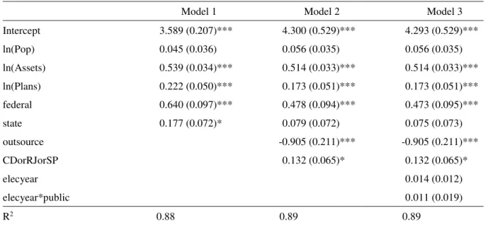
Table 8 presents estimation results of a model similar to Equation (4), but with two dummies (state and federal) instead of the public dummy. As in Tables 4 and 6, estimations use pooled ordinary least squares adjusted for clustering by group (EFPC). We see that after controlling for location and services outsourcing, the coefficient of the dummy for state government sponsor ceases to be statistically significant. However, the coefficient for federal government sponsor remains statistically significant at the 0.1% level.
Table 8
Cross-sectional Regression Estimates Separating Federal Sponsor
Model 1 Model 2 Model 3
Intercept 3.589 (0.207)*** 4.300 (0.529) *** 4.293 (0.529) ***
ln(Pop) 0.045 (0.036) 0.056 (0.035) 0.056 (0.035)
ln(Assets) 0.539 (0.034) *** 0.514 (0.033) *** 0.514 (0.033) ***
ln(Plans) 0.222 (0.050) *** 0.173 (0.051) *** 0.173 (0.051) ***
federal 0.640 (0.097) *** 0.478 (0.094) *** 0.473 (0.095) ***
state 0.177 (0.072) * 0.079 (0.072) 0.075 (0.073)
outsource -0.905 (0.211) *** -0.905 (0.211) ***
CDorRJorSP 0.132 (0.065) * 0.132 (0.065) *
elecyear 0.014 (0.012)
elecyear*public 0.011 (0.019)
R2 0.88 0.89 0.89
Note.This table reports the estimates of coefficients in a modified version of the econometric model of Equation (4), using pooled least squares regression adjusted for clusters by group (EFPC) on a balanced panel data with 820 observations (5 years by 164 individuals). Variables are defined in Table 1.
+ The values in parenthesis are the standard errors adjusted for clustering by group (EFPC). Significance levels are represented
by *** for 0.1%, ** for 1%, * for 5%, and . for 10%.
Table 9
Panel Estimates by Fixed Effects Method
ln(Pop) 0.257 (0.039) ***
ln(Assets) 0.390 (0.042) ***
ln(Plans) 0.110 (0.054) *
outsource -0.290 (0.117) *
elecyear 0.013 (0.013)
elecyear*federal 0.010 (0.030)
R2 0.28
Note. This table reports the estimates of coefficients in modified version of the econometric model expressed by Equation (5), using panel regression by fixed effects method on a balanced panel data with 820 observations (5 years by 164 individuals). Variables are defined in Table 1.
+ The values in parenthesis are the standard errors. Significance levels are represented by *** for 0.1%, ** for 1%, * for 5%,
and . for 10%.
Conclusions
Previous literature (Abi-Ramia, Boueri, & Sachsida, 2015; Bikker et al., 2012) reported that pension funds with public organizations as sponsors present greater administrative expenses. We investigated this sponsor bias, and presented evidence that it may be attributed, at least partially, to omitted variables, particularly variables to control for location and the level of services outsourcing by the pension funds. Indeed, for a subsample of medium-size pension funds, this sponsor bias ceases to be statistically significant, after we control for these effects. It also ceases, after controlling for these variables, if a state government organization is the sponsor; remaining essentially for EFPC with federal government as the sponsor. Both controls, for location and outsourcing level, were omitted by Abi-Ramia et al. (2015). The control for outsourcing level was omitted by Bikker et al. (2012), and in our analysis it appears more relevant to account for sponsor bias. Bikker et al. (2012) used a sample with pension funds from four countries, and used country dummies to control for location. However, the location within country may also be relevant, due to considerable differences in the cost of living. For this reason, we used a single dummy that controlled for location in one of the three regions with greater costs of living in Brazil.
The limitation of our approach, related to outsourcing level, is that we infer that greater outsourcing is related to misreporting of portfolio management expenses, but this can not be directly observed. An alternative conclusion is that closed pension funds sponsored by public organizations show suboptimal levels of service outsourcing.
We also tested whether the sponsor bias could be related to a political bias in the administration of pension funds. Bradley et al. (2016) and Carvalho (2014) relate political bias in the administration of public organizations with elections. Dinç (2005) more specifically presents changes of public organization behavior in election years. Following his idea, we tested whether there is evidence of an increase in administrative expenses by pension funds, especially public sponsored ones, in election years. Our findings do not support this political bias hypothesis. However, we could not test for continuous misuse of pension fund resources, such as continuous support to political parties.
from differences in the quality of management of administrative expenses, which are consistent with differences in structural characteristics between the two groups. Despite the fact that these groups are regulated by different legislation, it does not seem to affect the management of administrative expenses. As long as there is also no divergence in the quality of portfolio management, participants in public sponsored pension funds should not expect lower retirement payments (given the same flow of contributions) than participants in private sponsored pension funds.
References
Abi-Ramia, M., Boueri, R., & Sachsida, A. (2015). Economias de escala e escopo na previdência complementar fechada brasileira. Economia Aplicada, 19(3), 481-505. Retrieved from https://www.revistas.usp.br/ecoa/article/view/106044/104696
Almeida, A. N., & Azzoni, C. R. (2016). Custo de vida comparativo das regiões metropolitanas
brasileiras: 1996-2014. Estudos Econômicos (São Paulo), 46(1), 253-276.
http://dx.doi.org/10.1590/0101-416146128aaa
Associação Brasileira das Entidades Fechadas de Previdência Complementar. (2014, April). The Brazilian
pension system. Retrieved from
http://www.abrapp.org.br/Documentos%20Pblicos/The%20Brazilian%20Pension%20System.pdf
Bateman, H., & Mitchell, O. S. (2004). New evidence on pension plan design and administrative expenses: The Australian experience. Journal of Pension Economics and Finance, 3(1), 63-76. https://doi.org/10.1017/S1474747204001465
Bikker, J. A. (2017). Is there an optimal pension fund size? A scale-economy analysis of administrative costs. The Journal of Risk and Insurance, 84(2), 739-769. http://dx.doi.org/10.1111/jori.12103
Bikker, J. A., & De Dreu, J. (2009). Operating costs of pension funds: the impact of scale, governance, and plan design. Journal of Pension Economics and Finance, 8(1), 63-89. https://doi.org/10.1017/s1474747207002995
Bikker, J. A., Steenbeek, O. W., & Torracchi, F. (2012). The impact of scale, complexity, and service quality on the administrative costs of pension funds: A cross-country comparison. The Journal of Risk and Insurance, 79(2), 477-514. https://doi.org/10.1111/j.1539-6975.2011.01439.x
Bradley, D., Pantzalis, C., & Yuan, X. (2016). The influence of political bias in state pension funds. Journal of Financial Economics, 119(1), 69-91. https://doi.org/10.1016/j.jfineco.2015.08.017
Breusch, T. S., & Pagan, A. R. (1979). A simple test for heteroscedasticity and random coefficient variation. Econometrica, 47(5), 1287-1294. https://doi.org/10.2307/1911963
Brown, J. R., Pollet, J., & Weisbenner, S. J. (2009, September). The investment behavior of state pension plans [NBER Retirement Research Center Paper Nº NB 09-12]. National Bureau of Economic Research, Cambridge, MA, USA. Retrieved from http://www.nber.org/aging/rrc/papers/orrc09-12.pdf
Brown, J. R., Pollet, J. M., & Weisbenner, S. J. (2015, March). The in-state equity bias of state pension plans [NBER Working Paper Nº 21020]. National Bureau of Economic Research, Cambridge, MA, USA. Retrieved from http://www.nber.org/papers/w21020.pdf
Caswell, J. W. (1976). Economic efficiency in pension plan administration: A study of the construction industry. The Journal of Risk and Insurance, 43(2), 257-273. https://doi.org/10.2307/251979
Dinç, I. S. (2005). Politicians and banks: Political influences on government-owned banks in emerging
markets. Journal of Financial Economics, 77(2), 453-479.
https://doi.org/10.1016/j.jfineco.2004.06.011
Giannetti, M., & Laeven, L. (2009). Pension reform, ownership structure, and corporate governance: Evidence from a natural experiment. The Review of Financial Studies, 22(10), 4091-4127. https://doi.org/10.1093/rfs/hhn091
Hochberg, Y. V., & Rauh, J. D. (2013). Local overweighting and underperformance: Evidence from limited partner private equity investments. The Review of Financial Studies, 26(2), 403-451. https://doi.org/10.1093/rfs/hhs128
Khwaja, A. I., & Mian, A. (2005). Do lenders favor politically connected firms? Rent provision in an emerging financial market. The Quarterly Journal of Economics, 120(4), 1371-1411. https://doi.org/10.1162/003355305775097524
Lazzarini, S. G., Musacchio, A., Bandeira-de-Mello, R., & Marcon, R. (2015). What do state-owned development banks do? Evidence from BNDES, 2002–09. World Development, 66, 237-253. https://doi.org/10.1016/j.worlddev.2014.08.016
Lei n. 12.154, de 23 de dezembro de 2009. (2009). Cria a Superintendência Nacional de Previdência Complementar - PREVIC e dispõe sobre o seu pessoal; inclui a Câmara de Recursos da Previdência Complementar na estrutura básica do Ministério da Previdência Social; altera disposições referentes a auditores-fiscais da Receita Federal do Brasil; altera as Leis nos 11.457, de 16 de março de 2007, e 10.683, de 28 de maio de 2003; e dá outras providências. Retrieved from http://www.planalto.gov.br/ccivil_03/_ato2007-2010/2009/Lei/L12154.htm
Mitchell, O. S., & Andrews, E. S. (1981). Scale economies in private multi-employer pension systems. Industrial & Labor Relations Review, 34(4), 522-530. https://doi.org/10.2307/2522475
Petersen, M. A. (2009). Estimating standard errors in finance panel data sets: Comparing approaches. The Review of Financial Studies, 22(1), 435-480. https://doi.org/10.1093/rfs/hhn053
Ratcliffe, J. F. (1968). The effect on the t distribution of non-normality in the sampled population. Journal of the Royal Statistical Society. Series C (Applied Statistics), 17(1), 42-48. https://doi.org/10.2307/2985264
Sapienza, P. (2004). The effects of government ownership on bank lending. Journal of Financial Economics, 72(2), 357-384. https://doi.org/10.1016/j.jfineco.2002.10.002
Shapiro, S. S., & Wilk, M. B. (1965). An analysis of variance test for normality (complete samples). Biometrika, 52(3/4), 591-611. https://doi.org/10.2307/2333709
Superintendência Nacional de Previdência Complementar. (n.d.). Série de estudos número 6 – Divulgação das despesas administrativas das entidades fechadas de previdência complementar
– Exercício 2014. Retrieved from http://www.previc.gov.br/central-de-
conteudos/publicacoes/series-de-estudo/serie-de-estudos-1/6a-serie-de-estudos.pdf/@@download/file/6%C2%AA%20S%C3%A9rie%20de%20Estudos.pdf
Author’s Profile
Claudio Marcio Pereira da Cunha
APPENDIX
Regression Diagnostics
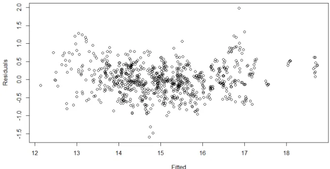
To analyze model misspecification, in Figure 1 we present a scatter plot of residuals against fitted values from Model 2 in Table 4. The random pattern observed does not indicate model misspecification, and is consistent with constant variance across fitted values. (Analogous plots for Models 1 and 3 in Table 4 are similar, but we do not present them to save space). To test for non-constant variance we apply the test proposed by Breusch and Pagan (1979) on the residuals of POLS. The null hypothesis (constant variance) is not rejected for any of the 3 models in Table 4, even considering confidence intervals greater than 10%.
Figure 1. Scatter Plot of Residuals Against Fitted Values from Model 2 in Table 4
Another usual concern in regression diagnosis is the independence of residuals. We expect explanatory variables of administrative expenses to be serially correlated. For instance, new closed pension funds present a growing trend in total assets, because there are few beneficiaries. Conversely, old funds may present more beneficiaries than active participants, implying a negative trend in total assets. Indeed, the Durbin-Watson and Breusch-Pagan tests for serial correlation reject the null hypothesis (absence of serial correlation) for less than 0.1% confidence intervals. For this reason we computed standard errors of estimated coefficients that are robust to serial correlation.
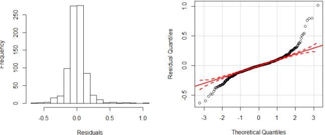
Because we have a reasonably large sample, with 820 observations in 164 groups (EFPC), normality of the distribution of residuals is not an issue, since Central Limit Theorem ensures the distribution of the estimators will converge asymptotically to a normal distribution. The speed of convergence, however, improves the closer to a normal distribution the residuals are (Ratcliffe, 1968). Figure 2 presents the histogram and the quantile-quantile (qq) plot, of residuals of Model 2 in Table 4. Both are compatible with the normal distribution, except for a few discrepant observations. (Analogous plots for Models 1 and 3 in Table 4 are similar, but we do not present them to save space.) Normality is usually tested using the test proposed by Shapiro and Wilk (1965). However, this test gets very sensible for large samples.
composed by observations grouped by year (to isolate the serial correlation effect), in a total of 5 subsamples (corresponding to years 2010 to 2014). For Model 2 in Table 4, we cannot reject the null hypothesis, with a 5% confidence level, in 4 of the 5 subsamples. With a 10% confidence interval, the null hypothesis is still not rejected for 3 of the 5 subsamples. Thus, from the patterns of the plots in Figures 2 and 3, and from the Shapiro-Wilk Test on the subsamples by year, we assume that the distribution of regression residuals does not differ significantly from the normal distribution, meaning that the t-tests we perform on the coefficient estimations are valid.
Figure 2. Histogram (Left) and Quantile-quantile (qq) Plot of Residuals from Model 2 in Table 4
In Tables 6, 7 and 8, as in Table 4, we run models that are variations of Equation (4), for different subsamples. As expected, because we are running the same model on samples from the same populations, the residual versus fitted, histogram and qq-plot are very similar to the ones presented above. Due to this similarity and to save space we do not present them here.
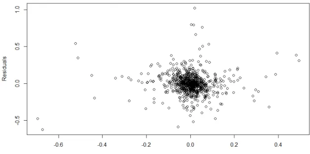
A different model is based on Equation (5). We also apply a different regression method, the fixed effects method for panel data. The residual versus fitted plot, computed from the parameters in Table 5, is presented in Figure 3, where we see more concentrated fitted values, because the method focuses on the variability over time (within). This practically eliminates the variability in the cross section of EFPC (between). However, the residuals still seem to follow a random pattern. Indeed, the Breusch-Pagan Test does not reject the null hypothesis of constant variance, even for confidence intervals greater than 10%.
In Figure 4 we see that the distribution of residuals present significant differences from the normal distribution, with a slight right skewness (0.9), and a high kurtosis (10.8). Because the convergence of means distribution to normal distribution, according to Ratcliffe (1968), is more affected by skewness, which is slight, than by kurtosis, we can still trust that the t-tests we perform on the coefficient estimations are valid.