An active contour model for the segmentation of images with intensity inhomogeneities and bias field estimation.

(1)

An Active Contour Model for the

Segmentation of Images with Intensity

Inhomogeneities and Bias Field Estimation

Chencheng Huang1,3, Li Zeng1,2*

1Key Laboratory of Optoelectronic Technology and System of the Education Ministry of China, Chongqing University, Chongqing, 400044, China,2College of Mathematics and Statistics, Chongqing University, Chongqing, 401331, China,3Engineering Research Center of Industrial Computed Tomography

Nondestructive Testing of the Education Ministry of China, Chongqing University, Chongqing, 400044, China *[email protected]

Abstract

Intensity inhomogeneity causes many difficulties in image segmentation and the under-standing of magnetic resonance (MR) images. Bias correction is an important method for addressing the intensity inhomogeneity of MR images before quantitative analysis. In this paper, a modified model is developed for segmenting images with intensity inhomogeneity and estimating the bias field simultaneously. In the modified model, a clustering criterion en-ergy function is defined by considering the difference between the measured image and es-timated image in local region. By using this difference in local region, the modified method can obtain accurate segmentation results and an accurate estimation of the bias field. The energy function is incorporated into a level set formulation with a level set regularization term, and the energy minimization is conducted by a level set evolution process. The pro-posed model first appeared as a two-phase model and then extended to a multi-phase one. The experimental results demonstrate the advantages of our model in terms of accuracy and insensitivity to the location of the initial contours. In particular, our method has been ap-plied to various synthetic and real images with desirable results.

Introduction

Image segmentation still plays an important role in image understanding and computer vision. Active contour models (ACMs) have been widely applied to image segmentation since their in-troduction [1]. ACMs can obtain closed object contours as segmentation results, which can be conveniently used for shape analysis and recognition. The active contours can utilize various types of prior knowledge, such as image intensity distribution information, boundary shape in-formation, and texture information [2–4], to obtain accurate results for object boundaries in image analysis.

ACMs can be categorized as edge-based models [5–8] or region-based models [9–15]. Edge-based models often use an image gradient to force the active contours to move toward the

OPEN ACCESS

Citation:Huang C, Zeng L (2015) An Active Contour Model for the Segmentation of Images with Intensity Inhomogeneities and Bias Field Estimation. PLoS ONE 10(4): e0120399. doi:10.1371/journal. pone.0120399

Academic Editor:Xuhui Huang, Hong Kong University of Science and Technology, HONG KONG

Received:August 21, 2014

Accepted:January 21, 2015

Published:April 2, 2015

Creative Commons Attribution License, which permits unrestricted use, distribution, and reproduction in any medium, provided the original author and source are credited.

Data Availability Statement:The original images (Fig. 1toFig. 12) are available on Figshare. The DOIs of the data arehttp://dx.doi.org/10.6084/m9. figshare.1300262. The original images inFig. 13can be download fromhttp://www.bic.mni.mcgill.ca/ brainweb/.

(2)

desired object’s boundaries. These models are typically sensitive to noise, and weak boundaries, which have small gradient values, may cause edge leakage. Region-based models use image sta-tistical information to attract the active contours to the object boundaries. They outperform edge-based models in many cases, such as computer tomography (CT) and magnetic resonance (MR) images. However, traditional region-based models rely on the idea that the intensity of images is homogeneous, which is not suitable for images with intensity inhomogeneity. For ex-ample, Chan and Vese proposed the Chan-Vese (CV) model [10], or piecewise constant (PC) model, under the assumption that an image consists of two statistically homogeneous regions and has a distinct mean pixel intensity in each region.

Intensity inhomogeneities often occur in real images, such as CT and MR images. Jungke et al. [16] illustrated that the most important problem for brain MR image segmentation is the occurrence of intensity inhomogeneities. Spatial intensity inhomogeneity are generally related to the properties of the MR image device and include static field inhomogeneity, bandwidth fil-tering of the data, eddy currents driven by field gradients, and especially radio frequency (RF) transmission and reception inhomogeneity [17]. The spatial intensity inhomogeneity caused many difficulties for MR image segmentation. Many research applications have been used for images with intensity inhomogeneity [2,4,18–22]. However, these methods do not consider the correction of the bias field, which is critical for particular clinical diagnoses. Many bias field correction methods have been widely studied in recent years [23–26]. The most popular meth-ods for bias field estimation are based on image segmentation [27–30]. In these methods, the bias field estimation and segmentation are performed simultaneously in each iteration to ob-tain a final optimal solution. To solve the segmentation problem of intensity inhomogeneity and estimate the bias field, Li et al. [29] proposed a novel variational level set model, that uses the weighted K-means clustering method to evaluate the bias field of image intensities in a neighborhood around each point in the image domain. By considering the retinex model [31], Li’s model can obtain accurate segmentation results and bias field estimates in the presence of intensity inhomogeneity, such as in MR and camera images. Some related methods, which have capabilities similar to Li’s model in terms of considering intensity inhomogeneity, have been proposed [2,18,30]. Zhang et al. proposed a locally statistical active contour model (LSACM) to segment images with intensity inhomogeneity and bias correction [32], which has good performance with bias correction. However, these models are sensitive to the location of the initial contours [33].

In this paper, we introduce the local regional difference to Li’s model. With this regional dif-ference, the modified model can improve both the accuracy of the segmentation results for im-ages with intensity inhomogeneity and the estimation of the bias field. We define a new local clustering criterion by collecting the local region difference in the entire image domain. Under this local clustering criterion, the bias field and segmentation results can be effectively cor-rected in each iteration for different initial contours. Experiments demonstrate that our model can obtain more accurate results.

The remainder of this paper is organized as follows. In the next section, we review some well-known region-based models and their limitations and then present our modified model and the numerical algorithm. The Results and Discussions section presents and discusses the experimental results. Finally, the Conclusions sections presents the conclusions of this study.

Models

The piecewise constant (PC) model

Chan and Vese proposed the CV model [10] to solve the segmentation of two-phase images whose mean intensities can be distinct. The main concept of the CV model is to search for a

no role in study design, data collection and analysis, decision to publish, or preparation of the manuscript.

(3)

particular partition of a given imageI(x) into two regions, one representing the objects to be detected and the other representing the background. For the given imageI(x), they proposed to minimize the following energy functional [10]

ECV_ð_C_;_c

1;c2Þ ¼l1

Z

inðCÞ

jIðxÞ c1j 2

dxþl2

Z

outðCÞ

jIðxÞ c2j 2

dxþnjCj; x2O: ð1Þ

whereλ1andλ2are positive constants,ν0,in(C) andout(C) represent the inner and outer

regions of the contourC, respectively, andc1andc2are two constants representing the mean

image intensities inin(C) andout(C), respectively, Thus, the CV model is also called the piece-wise constant (PC) model. Thefirst and second terms of (1) are the inner and outer datafidelity terms of the contourC, respectively. The third term of (1) is the length term, which is used to regularize the contourC. The CV model performs well in image segmentation due to its ability to detect objects whose boundaries are either smooth or not necessarily defined by a gradient and to obtain a larger convergence range; moreover, it is less sensitive to the initialization. However, when the intensities inside or outside of the curveCare not homogeneous, the con-stantsc1andc2may not accurately describe the variance in the local region; thus, the CV

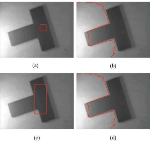
model may fail to segment images with intensity inhomogeneity (Fig. 1(b), (d)).

Li

_’

s model

Li et al. [29] considered the bias field in the local region to segment an image with intensity inhomogeneity and estimate the bias field. Based on the retinex theory [31], the considered

Fig 1. Segmentation of a real T-shaped image with intensity inhomogeneity by CV model.(a), (c) The original image with red initial contours. (b), (d) Segmentation results of the CV model.

(4)

bias field model can be written as follows:

I¼bJþn ð2Þ

whereIis an image to be measured,bis the biasﬁeld,Jis the true image andnis the additive noise. The assumptions for the true imageJand biasﬁeldbare as follows:

(A1) The bias fieldbvaries slowly over the entire image domain.

(A2) The true image intensitiesJare approximately constant within each class of issue, i.e.,J(x) ciforx2Oi, wherefOg

N

i_¼1is a partition ofO.

LetOx= {y:jy−xj ρ} be the neighborhood ofxin the image domain with a small radiusρ

andOx\Oirepresent the partition ofOxproduced by the i-th partitionOiof the image. Based on assumption (A1), the valueb(y) for allOxcan be close tob(x); then, in the small region

Ox\Oi, the product of the bias fieldb(y) and image intensityJ(y) can be an approximated byb (y)I(x)b(x)ciaccording to assumption (A2). By using the K-means clustering method, they considered all theNpartitions of image, and defined a local energy function as follows:

Ex ¼

XN

i¼1

Z

Ox\Oi

Ksðx yÞjIðyÞ bðxÞcij

2

dy ð3Þ

whereKσ(s) is a weighted function, which can be expressed as a Gaussian kernel function with standard deviationσ:

KsðsÞ ¼ 1

ffiffiffiffiffiffi 2_p p

se

jsj2 =2s2

; jsj<r

0_; _otherwise

ð4Þ 8 > < > :

Toﬁnd an optimal of the entire image domainO, an overall energy for allxis deﬁned as

E¼ Z

XN

i¼1

Z

Oi

2

dy

! dx

When considering the case in whichN= 2 in Li’s model, after introducing the level set function

ϕ(x), the overall energy can be written as

EðbðxÞ;c1;c2; ðxÞÞ ¼

Z X

2

i¼1

Z

O

2

dy

!

uiððxÞÞdx

whereu1(ϕ(x)) andu2(ϕ(x)) are the membership functions of each cluster,u1(s) =H(s), andH

(s) is the heaviside function deﬁned asHðsÞ ¼1 2½1þ

2

parctanð s

Þ( >0),u2(s) = 1−H(s). For

ﬁxedϕ,c1andc2, the optimal biasﬁeldbcan be computed by minimizing the local energyExin

(3)as follows:

b¼ Ks

X

2

i¼1

ciuiðÞ !

Ks X

2

i¼1

c2

iuiðÞ

(5)

where‘’denotes the convolution operation. Similarly, the optimalc1andc2can be computed

by

ci¼ R

ðKsbÞIuiðÞdx R

ðKsb

2

ÞuiðÞdx; i¼1;2 ð6Þ

In this case, the image domainOis divided into two regions,O1= {ϕ>0} (objects) andO2=

{ϕ<0} (background). Because the local image intensity information is embedded into the en-ergy function, Li’s method can address some types of images with intensity inhomogeneity; however, it still has inherent drawbacks. From(5)and(6), the intensity meansci(i= 1, 2) and biasﬁeldbare related; thus, the estimation ofc1andc2are critical for obtaining a better

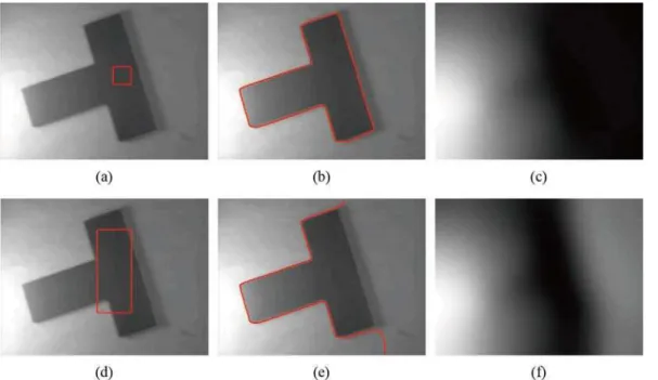
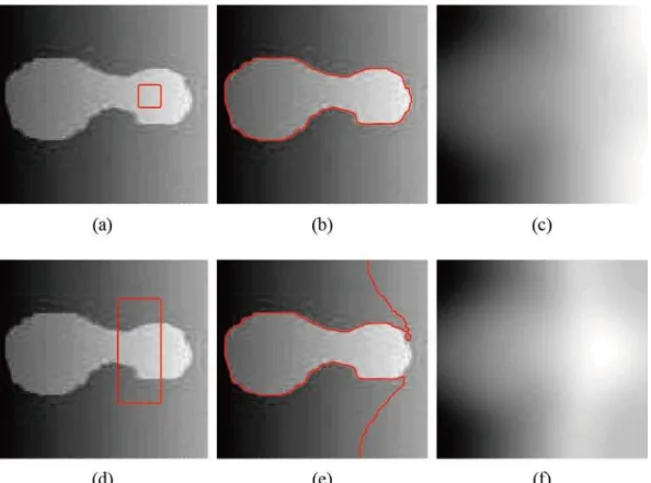
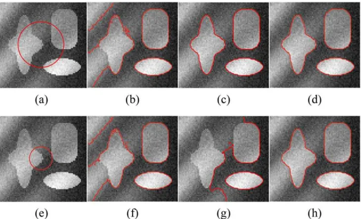
estima-tion of biasfieldb. However, when the object intensity is close to the background in the local region, the estimation of the biasfield may be inaccurate, and thus, estimating the biasfield using only the mean intensity in the local region is not sufficient. As shown inFig. 2, Li’s meth-od can obtain the correct segmentation (Fig. 2(b)) when the initial contour is located in the inner part of the object (Fig. 2(a)). However, when the initial contours contain both object and background (Fig. 2(d)), Li’s method fails to segment the object (Fig. 2(e)), and the false seg-mentation result leads to worse estimation of the biasfield (Fig. 2(f)). Similar results can also be seen inFig. 3. In other words, Li’s method may drop into local minimums [34] and is sensi-tive to the location of the initial contour; thus, the segmentation results and biasfield estima-tion may be inaccurate in some cases.

Our model

The segmentation result may affect the bias field correction, and using only the local region in-tensity means and bias field in Li’s model is not sufficient to approximate the measured image well. Thus, motivated by the contributions and methods of [27–30], we present a new ACM to segment images with intensity inhomogeneity and estimate the bias field, and this model

Fig 2. Segmentation of Li’s model.(a), (d) The original image with red initial contours. (b), (e) Segmentation results of Li’s model. (c), (f) The bias field estimation of Li’s model.

(6)

incorporates the local difference information between the measured image and Li’s estimate. In Li’s model, the segmentation result is essential for the estimation of the true imageJand the bias field; an accurate segmentation result can accurately estimate the bias field, whereas a bad segmentation result cannot do so. In our model, we introduce the difference in the local region of the image domain to improve the accuracy of the segmentation result and bias field estima-tion. For an input imageI, the model can be described as follows:

I¼bJþdþn ð7Þ

wheredis the difference between the measured imageIand approximated modelbJin the local region. According to this model, a K-means clustering-based local energy function of our model is deﬁned as follows:

Ex¼

XN

i¼1

Z

Ox\Oi

Ksðy xÞjIðyÞ bðxÞci dðxÞj

2

dy ð8Þ

whereKσ(s) is the Gaussian kernel function with standard deviationσ. By introducing the level set functionϕ(x) and considering all pixels in image domain, the overall energy can be written as

EðbðxÞ;c;dðxÞ; ðxÞÞ ¼

Z XN

i¼1

Z

O

Ksðx yÞjIðyÞ bðxÞci dðxÞj

2

dy

!

uiððxÞÞdx Fig 3. Segmentation of Li_’s model.(a), (d) The original image with red initial contours. (b), (e) The final segmentation results of Li’s model. (c), (f) The bias field estimation of Li’s model.

(7)

whereuiis the membership function andc= (c1,c2,. . .,cN). Afterfixingσ,candd, wefind an optimal biasfieldbthat minimizesExin(8):

b¼Ks ðI dÞ Jð

1_Þ

ð Þ

KsJð

2_Þ ð9Þ

where‘’is the convolution operation,Jð1_Þ

¼PN i¼1

ciuiðÞandJð

2_Þ

¼PN i¼1

c2

iuiðÞ,ui(ϕ) is the mem-bership function of the partitionOi. Similarly, the optimalcanddcan be obtained from(8):

ci ¼ R

ðKsbÞðI dÞuiðÞdx R

ðKsb

2

ÞuiðÞdx

; i¼1_{; :::;}_N

d ¼KsMð

1_Þ

KsMð

2_Þ

ð10Þ

whereMð1_Þ

¼PN i¼1

IuiðÞ bciuiðÞ

ð ÞandMð2_Þ

¼PN i¼1

uiðÞ.

In the process of curve evolving (the zero level set function), we keep the level set function as an approximate signed distance function, especially in the neighborhood of the zero level set [35]. For a general level set function method, the level set function is often computed as a signed distance function and must re-initialize the level set function after some evolution steps, but the re-initialization step is time-consuming and not effective. Li et al. proposed a regulari-zation term [36] as a penalty term to eliminate the re-initialization step. The regularization term can be written as follows:

PðÞ ¼1₂ Z

O

ðjrðxÞj 1Þ 2

dx

This regularization term can force the level set function to be closed to a signed distance func-tion in the process of curve evolufunc-tion. We also choose the length term in the CV model for more accurate computation, so a regularization term can be written as

ER_ð_{Þ ¼}_a Z

O

1

2ðjrðxÞj 1Þ

2

dxþb

Z

O

jrHððxÞÞjdx

Theﬁnal energy functional can be written as follow

EFEF_ðb_;

c;d; Þ ¼Eðb;c;d; Þ þERðÞ ð11Þ

The level set variation formulation of our model

In level set methods, the evolving contour (object contours) is represented by zero level set functionϕ= 0 in the level set formulation. The case ofN= 2 andN>2 in the energy represents two-phase and multi-phase formulations, respectively. In the following subsections, we will consider two-phase and multi-phase cases.

Two-phase level set variation formulation. For two-phase (N = 2) images, which the whole image domainOcontains foreground and background. The energy functional can be written as follows:

EFEF_ð_b_;

c;d; Þ ¼

Z X

2

i¼1

Z

Ksðy xÞjIðyÞ bðxÞci dðxÞj

2

uiðÞdy

!

(8)

whereu1andu2are the membership functions ofO1andO2,b,c1,c2anddare given as follows:

b¼

Ks ðI dÞ X

2

i¼1

ciuiðÞ !

Ks X

2

i¼1

c2

iuiðÞ

ci ¼ R

ðKsbÞðI dÞuiðÞdx R

ðKsb

2

ÞuiðÞdx ; i¼

1_;2

d¼ Ks

X

2

i¼1

ðI bciÞuiðÞ

ð Þ

Ks X

2

i¼1

uiðÞ

ð13Þ

Note 1: The differencedis a matrix with dimensionM×N([M, N]=size(I)). If the local dif-ference matrixd= 0, our method is similar to Li’s method in [29]; however, there are still dif-ferences even for an accurate approximating evaluation of the measured image. Thus, ford6¼ 0, the local difference variable between imageI(x) and the approximate formb(y)ciin each Ox\Oican be corrected in our model. If there is a largedin the local region ofx, the measured imageI(x) is not well approximated by the local bias field and local piecewise constant, and the active contours will move to the regions that reduced. Thus, the proposed method will obtain more accurate results in each iteration because the local difference in each clustering of the image is considered.

Note 2: Wherever the region’s initial contours are located, the differencedcan always be collected in each local region and corrected by the estimatebandcito the smaller values be-tween the measured image and approximatebci, which makes our model insensitive to the ini-tialization of the active contour.

Note 3: The size of the Gaussian window is also important for accurate segmentation and bias field correction. In our experiment, we choose a truncated Gaussian window of size (4k +1)×(4k+1), wherekis the greatest integer smaller thanσ. Thus, the choice ofσis related to the size of the Gaussian window.

In order to facilitate the numerical simulation, we use the membership functionsu1(s) =

H(s) andu(s) = 1−H(s), whereHðsÞ ¼

1 2ð1þ

2

parctanð s

ÞÞis the smooth version of Heaviside function anddH_dsðsÞ¼1

p 2

þs2¼dðsÞ. By using the gradient flows method [37], the formulation of the variation equation with the level set function of(12)can be written as

@

@t ¼dðÞðf2 f1Þ þa r 2

div r

jrj

þbdðÞ div r

jrj

ð14Þ

where:

f1¼

Z

Kðy xÞjIðxÞ bðyÞc1 dðyÞj 2

dy

f2¼

Z

(9)

andb,cianddare given by(13). The corresponding initial condition and boundary condition are as follows:

ðx;0Þ ¼0ðxÞ; x2O @

@n¼

0_; _x₂_@_O ð15Þ

wherendenotes the exterior normal to the image boundary@O.

We use the explicit finite difference scheme to discretize the level setEquation (14)as fol-lows:

kþ1 k Dt ¼dð

k

Þðf2 f1Þ þa r 2

k

div r k

jrk j

þbdðk

Þ div r k

jrk j

ð16Þ

whereϕkrepresents the values of the level set function in the k-th iteration andΔtis the time step of the evolving contours.

Multi-phase level set variation formulation. For the caseN>2, we can obtain the multi-phase level set formation similar to the caseN= 2. The difference is that we need to usenlevel set functionϕ1,ϕ2,. . .,ϕnto respectN= 2nregionsO1,O2,. . .,ON. The corresponding mem-bership functionsuican be written as

uið1ðxÞ; 2ðxÞ; :::; nðxÞÞ ¼

1_; _x₂_O

0_; _else

ð17Þ (

We denoteF= (ϕ1(x),ϕ2(x),. . .,ϕn(x)) for simplicity and he membership functionui(ϕ1(x), ϕ2(x),. . .,ϕn(x)) can be written asui(F). We focus on the caseN= 3 in this paper, which two level set functionsϕ1andϕ2can be used to deﬁne the partitions of image domain by the

mem-bership functionsu1(F) =H(ϕ1)H(ϕ2),u2(F) =H(ϕ1)(1−H(ϕ2)) andu3(F) = 1−H(ϕ1).

Similar to the two-phase case, theﬁnal energy of the multi-phase image can be written as

EFEF

ðb;c;d;FÞ ¼

Z X

3

i¼1

Z

Ksðy xÞjIðyÞ bðxÞc_i dðxÞj2u_iðFÞdy

!

dxþERðFÞ ð18Þ

whereb,c, anddcan be calculated from(13). Minimization of the energy functional inEquation (18)with respect toF= (ϕ1,ϕ2), we obtain the following gradient descentﬂow equations:

@1

@t ¼dð1Þ ðð f2 f1ÞHð2Þ þf3 f2Þ þa r

2

1 div r1

jr1j

þbd_ð1Þ div r1

jr1j

ð19Þ

@2

@t ¼dð2Þ ðð f2 f1ÞHð1ÞÞ þa r 2

2 div

r2

jr2j

þbd_ð2Þ div

r2

jr2j

ð20Þ

f1¼

Z

dy

f2¼

Z

dy

f3¼

Z

(10)

The numerical algorithm can be written as the following 6 steps (take the three-phase case for example):

1. Setk= 1 and initialize the level set functionsϕ1andϕ2to be binary functions

1ðx;0Þ ¼

c0; x2R1;

c0; x2= R1:

2ðx;0Þ ¼

c0; x2R2;

c0; x2= R2:

8 <

: 8

<

:

wherec0is a positive constant,R1andR2are arbitrarily given regions in the image domain.

2. Initialize the bias fieldband local difference matrixd.

3. Computeb,canddfrom(13).

4. Solve the level set functionϕ1from(19).

5. Solve the level set functionϕ2from(20).

6. Check whether the evolution is converged. If not, setk=k+1 and return to step 3.

Performance evaluations

In this paper, we use the jaccard similarity (JS) [17,38], the dice similarity coefficient (DSC) [17,39], the false positive ratio (RFP), and the false negative ratio (RFN) to compare the seg-mentation performances of the models quantitatively. These metrics are defined as:

JS ¼NðSg T

SmÞ NðSg

S

SmÞ; DSC¼ 2_N_ð_S

g T

SmÞ NðSgÞ þNðSmÞ

RFP ¼NðSg=OÞ

NðSgÞ ; RFN¼

NðSm=OÞ NðSmÞ

ð21Þ

whereN() represents the pixel numbers of the region.Sgindicates the foreground of the ground truth image andSmstands for the foreground obtained by the models.Ois the common part of SgandSm. The closer the JS and DSC values to 1, and the RFP and RFN values to 0, the better the segmentation results.

Statistical Analysis

Statistical analysis is performed using the statistical software MedCalc [40]. To assess the per-formance evaluations of segmentation quality (JS, DSC, RFP, RFN) presented in(21), the tests of statistical significance are performed using 120 simulated MR images. First, we perform the F-test [41]. If the associated (two-sided) P-value is less than the conventional 0.05, the null hy-pothesis is rejected and the conclusion is that the two variances do indeed differ significantly. If the P-value is low (P<0.05), the variances of the two samples cannot be assumed to be equal and it should be considered to use the t-test with a correction for unequal variances (Welch t test, [42]). The variables are expressed as Mean ± SD (standard deviations). For Welch t test, when the P-value is less than the conventional 0.05, the null hypothesis is rejected and the con-clusion is that the two means do indeed differ significantly.

Results and Discussion

(11)

programming environment on a personal computer with an Intel Core 2 Duo 2.80 GHz CPU, 4 GB RAM, and Windows 7 (64bit) operating system. In our experiments, we use the following default settings of the parameters for our method unless otherwise specified:σ= 3 (3σ 10),= 1, time stepΔt= 0.1,α= 0.1/Δt, andβ= 0.003 × 255 × 255. Most of the original images in experiments can be found at the websitehttp://www.engr.uconn.edu/~cmli/.

The next experiment considers the segmentation of the same image inFig. 1(as shown in Fig. 4). The T-shaped image is a real image with intensity inhomogeneity, which size is 127×96. The initial active contours are set inside the object domain and contain the background. Our method outperforms Li’s model (the code was downloaded from [44]) in some cases. As the local regional difference is considered, incorrect estimations of the true imageJin the local re-gion can be corrected in each iteration, which is insensitive to the initial contours in our experi-ments.Fig. 4indicates that even the initial contours located inside the objects contain

background, the segmentation results and bias field estimate are nearly the same. We choose the absolute value of the local differenced, which is shown in gray images (Fig. 4(c)andFig. 4 (g)) to describe the level between the measured imageIand estimatedbJ. In Figs.4(c) and 4(g), jdjis often large in highlight regions or regions with similar intensities; in these regions, the dif-ference betweenIandbJmust be corrected to obtain better estimations ofbandJ. By the quan-titative comparison using the above metrics in the second row ofFig. 2andFig. 4, the values of JS and DSC in our method are bigger than Li’s method, the value of RFP are equal show that the regionSb/Oof Li’s method and our method are the same, while the value of RFN in our model (0.0068) are smaller than Li’s method (0.3186) mean the regionSm/Oof our method achieves more accurate segmentation results (seeTable 1).

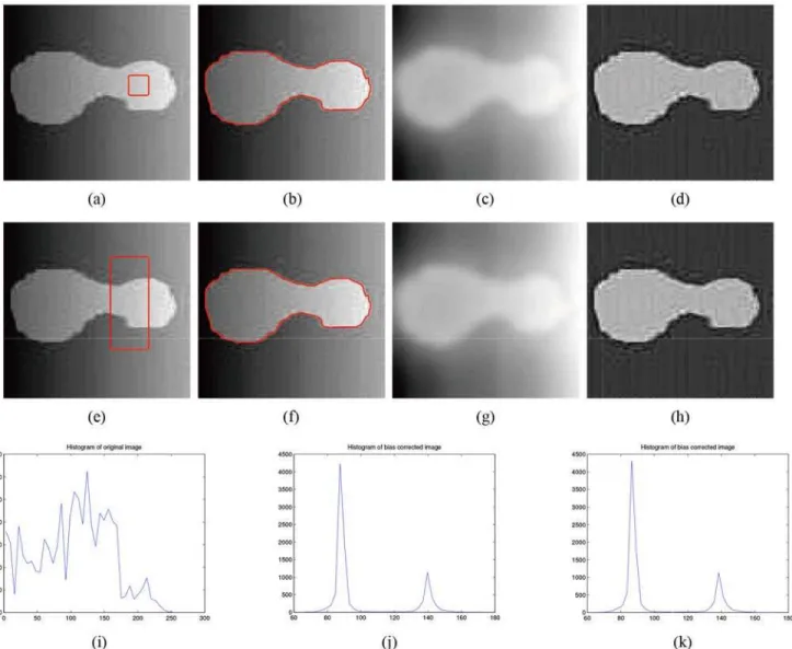
Fig. 5shows the segmentation results and bias field correction of the synthetic image with intensity inhomogeneity shown inFig. 3obtained by our model. For the distinct initial con-tours in Figs.5(a) and 5(e), the corrected images are shown in Figs.5(d) and 5(h), and the his-tograms of bias corrected image for different initial contours are shown inFig. 5(j) and 5(k),

Fig 4. Experimental results of our model.(a), (e) The original image with red initial contours. (b), (f) The final segmentation results of our model. (c), (g) The gray images ofjd_j_{. (d), (h) The estimation of the bias field in our model.}

(12)

which results in higher-quality image than the original image (Fig. 5(g)). The two histograms of the bias-corrected image with different initial contours are nearly identical.

Fig. 6shows the segmentation results for a synthetic image (the image size is 79×75) with higher intensity inhomogeneity obtained with Li’s method, LSACM (code can be downloaded at [45]) and our model. In this experiment, we choseβ= 0.007×255×255. The image contains

Table 1. JS, DSC, RFP and RFN values for the results in the second row ofFig. 2andFig. 4.

JS DSC RFP RFN

Li’s method 0.6782 0.8082 0.0047 0.3186

Our method 0.9864 0.9903 0.0047 0.0068

doi:10.1371/journal.pone.0120399.t001

Fig 5. Experimental results of our model.(a), (e) The original image with red initial contours. (b), (f) The final segmentation results of our model. (c), (g) The estimation of the bias field. (d), (h) The corrected image. (i) The histogram of the original image. (j) The histogram of the corrected image with initial contour (a). (k) The histogram of the corrected image with initial contour (e).

(13)

three objects with high light on the left, and the light also causes the boundary to be fuzzy in the lower region of the star-shaped object. For Li’s method, the estimation of the true imageJ (piecewise constants) may not be accurate in the fuzzy boundary region, and thus, the estima-tion of the bias field may also not be accurate. The segmentaestima-tion results obtained with Li’s method, LSACM and the proposed method for different initial contours are shown in columns 2, 3 and 4, respectively. Li’s method fails to segment the object boundary or estimate the fuzzy bias field with high light even when the initial contour across three objects. While LSACM can obtain the right segment result for the initial contour shown inFig. 6 (a), but for the initial con-tour asFig. 6 (e), LSACM get the undesired results even the iterate number over than 2000. The experimental results of our method are more accurate than those obtained with Li’s meth-od and more robustness than LSACM. In Figs.6(d) and 6(h), the final contours of our method can converge to the correct boundaries precisely. The bias field estimation and corrected image of Li’s model, LSACM and our model are shown inFig. 7. In the highlight region of the image, the image is not well corrected by Li’s method, LSACM and our method have the similar bias field estimation based on the right segmentation.

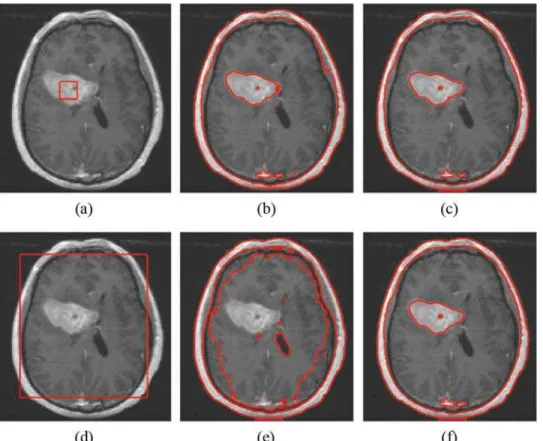
The quality of MR images is highly dependent upon the coil used to receive the RF signal emitted from the patient [43].Fig. 8shows the comparison between Li’s method and our meth-od for the segmentation results with different initial contours of an MR brain image (the size is 109×119) with a tumor from the Internet. A small black spot is located at the center of the tumor. The first row shows the segmentation results with the initial contour ofFig. 8(a), and the second row shows the results with the initial contour ofFig. 8(d). Columns 1 to 3 are the

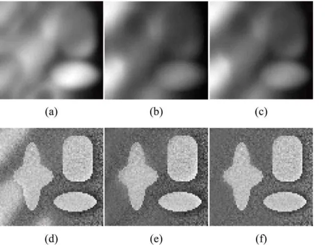
Fig 6. Comparisons of the segmentation results for a synthetic image with intensity inhomogeneity between Li’s model, LSACM and our model.

(a), (e) The original image with red initial contours. (b), (f) The results of Li’s model. (c), (g) The results of LSACM. (d), (h) The results of our model.

(14)

original image with red initial contours, the segmentation results of Li’s method and the results of our method, respectively. Li’s method fails to acquire the tumor and spot boundaries with the initial contour shown inFig. 8(a). The tumor boundaries obtained by Li’s model are inaccu-rate when the initial contour lies inside the tumor (Fig. 8(d)). Our method can obtain the boundaries of the tumor and small spot accurately because it collects the local regional differ-ence in the entire image domain.

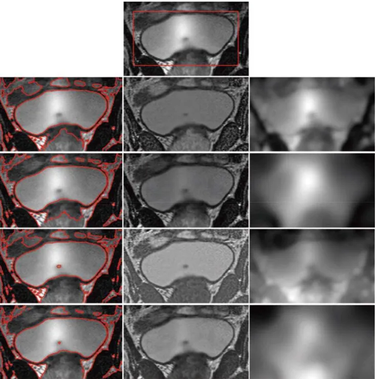
To test the impaction of the segmentation results and corrected images for differentσin the Gaussian kernel function, we compare the experimental results for an MR image obtain from Li’s method and our method with differentσ. From assumption (A1), the local region differ-encedwill be more accurately collected when the size of the Gaussian window is small. Thus, in this case, more details can be considered, and the segmentation may contain more details. In contrast, choosing a larger Gaussian window size may lead to a less accurate segmentation re-sult and increased computational. To record the computational cost for each method, we set the iteration numbern= 200.Fig. 9shows the comparison between Li’s method and our meth-od with different scalesσ= 3, 10. The original MR image with the initial contour is shown in the first row ofFig. 9, the size of the image is 180×107, and columns 1, 2 and 3 provide the final segmentation results, the estimated bias field and the corrected images, respectively. Rows 2 and 3 are the final results by Li’s method, and rows 4 and 5 are the results of our method; rows 2 and 4 consider the scaleσ= 3, whereas rows 3 and 5 considerσ= 10.Fig. 9illustrates that Li’s

Fig 7. Comparisons of the bias field estimation and corrected image forFig. 6between Li’s model, LSACM and our model.(a), (b), (c) The estimated bias fields of Li’s model, LSACM and our model, respectively. (d), (e), (f) The corrected images of Li’s model, LSACM and our model, respectively.

(15)

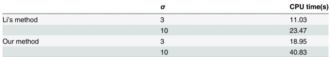
method fails to segment the small gray object at the center of the MR image forσ= 3 andσ= 10. Our method can accurately segment the small object in the image for the scaleσ= 3 and segment the small object in further detail whenσ= 10. Furthermore, the corrected images ob-tained with our method are superior to those obtain with Li’s method.Fig. 9also shows that the corrected image of our method obtained whenσ= 3 is better than that obtained whenσ= 10; thus, the results may be more accurate for smallerσthan in for largerσ.Table 2compares the CPU time for Li’s model and our model for different scalesσ. The CPU time forσ= 10 is approximately twice that of scaleσ= 3. Our model is more computationally burdensome than Li’s model because of the local regional difference estimation in each iteration.

For the observed image synthesized from the retinex model [31], we compare the perfor-mance of Li’s model, LSACM and our model for two synthesize images (which sizes are 50×50 and 64×61) multiplied by bias fields shown inFig. 10. Column 1 inFig. 10shows the synthesize images (row 1 and row 4), the corresponding multiplicative bias fields (row 2 and row 5) and the initial contours for the multiplied images (row 3 and row 6), respectively. Column 2 to 4 shows the segment results, the estimated bias fields and the corrected images. Rows 1 and 4 are the results of Li’s model, rows 2 and 5 show the results of LSACM, and rows 3 and 6 are the re-sults of our model. As shown inFig. 10, three models can obtain similar bias fields under the premise of right segmentations (rows 1, 2 and 3). However, for the initial contour shown in row 6 (column 1), the estimated bias field of our model are more similar to the given bias field than other two models (rows 4, 5 and 6). That is to say, our model may show better perfor-mance than Li’s model and LSACM in this statement.

Fig 8. Comparisons of the segmentation results for a MR brain image contains tumor with intensity inhomogeneity between Li’s model and our model.(a), (d) The original image with initial contours. (b), (e) The results of Li’s model. (c), (f) The results of our model.

(16)

In the following experiments, we compare our model with Li’s model [29] and LSACM [30] (the code was downloaded from [45]) in the performance of multi-phase MR images.Fig. 11 shows the segmentation and bias-correction results on 3T MR image (from [45], the image size is 174×238), which contains white matter (WM), gray matter (GM), cerebrospinal fluid (CSF) and background (CSF usually as the background in our method). We use red contour to

Fig 9. Comparisons of Li’s model and our model in different scaleσon MR image.Row 1 is the original image with red initial contours. The first column

is the final segmentation results. The second column is the estimated bias field images. The third column is the corrected images. Row 2 and 3 are the corresponding results of Li’s model inσ= 3 andσ= 10. Row 4 and 5 are the final results of our model inσ= 3 andσ= 10 respectively.

(17)

representϕ1= 0, and blue to representϕ2= 0. The first column shows the original image and

initial contours, the second column shows the segmentation results, the third and fourth col-umns show the corrected images and bias fields, respectively. The first, second and third rows show the results of Li’s method, LSACM and our method, respectively. As we see fromFig. 11, our method and LSACM capture more CSF than Li’s method and our method obtain more ac-curacy of GM (WM) in the center of image than other two methods. The corrected images of LSACM and our method seem similar, which are better than Li’s method. For the brain MR image inFig. 12, the original image (the image size is 141×202) and initial contours are shown in column 1, row 1, 2 and 3 are the results of Li’s method, LSACM and our method, respective-ly. LSACM can obtain the accurate boundaries of WG (blue contours), but the segmentation of CSF is unexpected (red contours), which can not be well separated the WM and GM. Li’s meth-od can not segment the GM in the center of image.Fig. 11andFig. 12show that our method have more capacity of WM and GM segmentation. The corrected images of Li’s method and our method seem similar and more vivid than LSACM.

To further support the conclusion statements, we compare the performance of WM and GM segmentation of simulated MR image volumes for normal brain (the data can be download from [46], the image size of each slice is 217×181). We use 120 slices, which contain both WM and Gm for comparison. As shown inFig. 13, three original images are shown in column 1, col-umn 2 shows the ground truth of WM and GM, colcol-umn 3 to 5 shows the results of Li’s method, LSACM and our method, respectively. Rows 1, 3 and 5 are WM, and rows 2, 4 and 6 are GM, all WM and GM are displayed in white. As mentioned above, we first perform the F-test. Since the P-values are lower than 0.05, the variances of these samples cannot be assumed to be equal. We need to perform the Welch’s t test. The statistical analysis results of performance evalua-tions of segment accuracy for WM and GM between different method are summarized in Table 3andTable 4, respectively. The variables are expressed as Mean±SD. FromTable 3, there are obvious statistical differences of JS values between Li’s method and LSACM (P<0.0001), Li’s method and our method (P = 0.0022). The values of JS for LASM (0.7146 ±0.0091) and our method (0.6994±0.0175) is higher than Li’s method (0.6560±0.0060). There is no obvious statistical difference in the value of JS between LSACM and our method

(P = 0.3095>0.05). There are obvious statistical differences of DSC values between Li’s method and LSACM (P = 0.0001), LSACM and our method (P = 0.0003). The value of DSC for our method (0.8620±0.0019) is higher than Li’s method (0.8140±0.0141) and LSACM (0.8286 ±0.0081). There is no obvious statistical difference in the value of DSC between LSACM and Li’s method (P = 0.2826>0.05). There is no obvious statistical difference of RFP between Li’s method and LSACM (P = 0.0948>0.05), LSACM and our method (P = 0.6486>0.05). There is obvious statistical difference in the of RFP between Li’s method and our method

(P = 0.0454<0.05). The value of RFP for our method (0.1598±0.0012) is lower than that of Li’s method (0.1714±0.0028). There is no obvious statistical difference in the value of RFN between Li’s method and LSACM (P = 0.3407>0.05). There is obvious statistical difference of RFN be-tween Li’s method and our method (P<0.0001), LSACM and our method (P<0.0001). The

Table 2. Comparison the CPU time of Li’s method and our method forFig. 9.

σ CPU time(s)

Li’s method 3 11.03

10 23.47

Our method 3 18.95

10 40.83

(18)

Fig 10. Comparisons of Li’s model, LSACM and our model for two synthesize images multiplied by given bias fields.Column 1 is the original images (row 1, 4), given bias fields (row 2, 5) and the initial contours in the images multiplied by bias fields (row 3, 6). Column 2 to 4 is the segmentation results, estimated bias fields and corrected images, respectively. Row 1 and 4 are the results of Li’s model. Row 2 and 5 are the results of LSACM. Row 3 and 6 are the results of our model.

(19)

value of RFN for our method (0.1130±0.0041) is lower than Li’s method (0.1876±0.0238) and LSACM (0.1710±0.0127). FromTable 4, there are obvious statistical differences in the values of JS and DSC between any two methods of Li’s method, LSACM and our method (the minimized P = 0.0137). And the values of JS and DSC for our method (JS: 0.6842±0.0014, DSC: 0.8608 ±0.0004) are significantly higher than that of Li’s method (JS: 0.6442±0.0048, DSC: 0.7814 ±0.0028) and LSACM (JS: 0.6137±0.0132, DSC: 0.7534±0.0107). There is no obvious statistical

Fig 11. Comparisons of Li’s model, LSACM and our model for MR brain image.Column 1 is the original image with red and blue initial contours. Column 2 to 4 is the final segmentation results, the corrected images and the estimated bias field images, respectively. Row 1 to 3 is the results of Li’s model, LSACM and our model, respectively.

(20)

Fig 12. Comparisons of Li’s model, LSACM and our model for MR brain image.Column 1 is the original image with red and blue initial contours. Column 2 to 4 is the final segmentation results, the corrected images and the estimated bias field images, respectively. Row 1 to 3 is the results of Li’s model, LSACM and our model, respectively.

(21)

Fig 13. Comparisons of the segmentation results for WM and GM among Li_’s model, LSACM and our model.Column 1 are the original images. Column 2 is the ground truth of original images. Column 3 to 5 is the final segmentation results of Li’s method, LSACM and our method, respectively. Rows 1, 3 and 5 are WM, and rows 2, 4 and 6 are GM. All WM and GM are displayed in white.

(22)

differences in the value of RFP between Li’s method and LSACM (P = 0.9731>0.05), LSACM and our method (P = 0.0511>0.05). And there is obvious statistical differences in the value of RFP between Li’s method and our method (P = 0.0337). The value of RFP for our method (0.1293±0.0007) is significantly lower than that of Li’s method (0.1360±0.0005). There are ob-vious statistical differences in the values of RFN between any two methods of Li’s method, LSACM and our method (the minimized P = 0.0080). And the value of RFN for our method (0.1480±0.0008) is significantly lower than that of Li’s method (0.2826±0.0065) and LSACM (0.3200±0.0170).

Conclusions

In this paper, we developed a new model for image segmentation with intensity inhomogeneity and bias field estimation. We firstly defined a local intensity clustering criterion function by considering the local difference between the measured image and estimated image. Then, the energy is minimized by a level set evolution process. A regularization is used in the level set process to ensure that the active contours are smooth and eliminate the re-initialization of level set function in the evolution of the active contours. We further extend our model into a multi-phase one to segment multi-multi-phase images to segment WM and GM in the simulated normal brain MR image volumes. For 120 MR image slices, our method outperforms Li’s method in terms of JS, DSC, RFP and RFN for WM and GM. Our method outperforms LSACM in terms of DSC and RFN for WM, JS, DSC and RFN for GM. Our method can obtain accurate segmen-tation results and accurate estimations of the bias field. Experimental results on synthetic and real images demonstrate that our model is efficient.

Author Contributions

Conceived and designed the experiments: LZ CCH. Performed the experiments: CCH. Ana-lyzed the data: CCH. Contributed reagents/materials/analysis tools: LZ CCH. Wrote the paper: CCH.

Table 3. Summary of Welchs t test analysis results of performance evaluations of WM segmentation quality between different methods (for 120 simulated MR image slices of the normal brain).

Li’s method (A) LSACM (B) Our method (C) P-value

A vs. B A vs. C B vs. C

JS 0.6560±_0.0060 _0.7146±_0.0091 _0.6994±_0.0175 _<_0.0001 _0.0022 _0.3095

DSC 0.8140±0.0141 0.8286±0.0081 0.8620±0.0019 0.2826 0.0001 0.0003

RFP 0.1714±0.0028 0.1618±0.0011 0.1598±0.0012 0.0948 0.0454 0.6486

RFN 0.1876±_0.0238 _0.1710±_0.0127 _0.1130±_0.0041 _0.3407 _<_0.0001 _<_0.0001

doi:10.1371/journal.pone.0120399.t003

Table 4. Summary of Welchs t test analysis results of performance evaluations of GM segmentation quality between different methods (for 120 simulated MR image slices of the normal brain).

Li’s method (A) LSACM (B) Our method (C) P-value

A vs. B A vs. C B vs. C

JS 0.6442±_0.0048 _0.6137±_0.0132 _0.6842±_0.0014 _0.0137 _<_0.0001 _<_0.0001

DSC 0.7814±0.0028 0.7534±0.0107 0.8608±0.0004 0.0091 <0.0001 <0.0001

RFP 0.1360±0.0005 0.1359±0.0007 0.1293±0.0007 0.9731 0.0337 0.0511

RFN 0.2826±0.0065 0.3200±0.0170 0.1481±0.0008 0.0080 <0.0001 <0.0001

(23)

References

1. Kass M, Witkin A, Terzopoulos D (1988) Snakes: active contour models. International Journal of Com-puter Vision 1: 321–331. doi:10.1007/BF00133570

2. Li, CM, Kao, CY, Gore, JC, Ding, ZH (2007) Implicit active contours driven by local binary fitting energy. IEEE Conference on Computer Vision and Pattern Recognition: 1–7.

3. Xu CY, Prince JL (1998) Snakes, shapes, and gradient vector flow. IEEE Transactions on Image Pro-cessing 7: 359–369. doi:10.1109/83.661186PMID:18276256

4. Wang X, Huang D, Xu H (2010) An efficient local Chan-Vese model for image segmentation. Pattern Recognition 43: 603–618. doi:10.1016/j.patcog.2009.08.002

5. Caselles V, Catte F, Coll T, Dibos F (1993) A geometric model for active contours in image processing. Numerische Mathematik 66: 1–31. doi:10.1007/BF01385685

6. Malladi R, Sethian JA, Vemuri BC (1995) Shape modeling with front propagation: a level set approach. IEEE Transactions on Pattern Analysis and Machine Intelligence 17: 158–175. doi:10.1109/34. 368173

7. Kichenassamy S, Kumar A, Olver P, Tannenbaum A, Yezzi A (1995) Gradient flows and geometric ac-tive contour models. Fifth International Conference on Computer Vision: 810–815.

8. Vasilevskiy A, Siddiqi K (2002) Flux maximizing geometric flows. IEEE Transactions on Pattern Analy-sis and Machine Intelligence 24: 1565–1578. doi:10.1109/TPAMI.2002.1114849

9. Ronfard R (1994) Region-based strategies for active contour models. International Journal of Computer Vision 13: 229–251. doi:10.1007/BF01427153

10. Chan T, Vese L (2001) Active contours without edges. IEEE Transaction on Image Processing 10: 266–277. doi:10.1109/83.902291

11. Paragios N, Deriche R (2002) Geodesic active regions and level set methods for supervised texture segmentation. International Journal of Computer Vision 46: 223–247. doi:10.1023/A:1014080923068

12. Vese L, Chan T (2002) A multiphase level set framework for image segmentation using the Mumford and Shah model. International Journal of Computer Vision 50: 271–293. doi:10.1023/

A:1020874308076

13. Li W, Hu XP (2013) Robust Tract Skeleton Extraction of Cingulum Based on Active Contour Model from Diffusion Tensor MR Imaging. PloS one 8.

14. Liao XY, Tuan ZY, Zheng Q, Yin Q, Zhang D, Zhao JH (2014) Multi-Scale and Shape Constrained Lo-calized Region Based Active Contour Segmentation of Uterine Fibroid Ultrasound Images in HIFU Therapy. PloS one 9.

15. Liu LH, Zeng L, Luan X (2013) 3D robust Chan-Vese model for industrial computed tomography volume data segmentation. Optics and Lasers in Engineering 51: 1235–1244. doi:10.1016/j.optlaseng.2013. 04.019

16. Jungke M, Seelen WV, Bielke G, Meindl S, Grigat M, Pfannenstiel P (1988) A system for the diagnostic use of tissue characterizing parameters in NMR-tomography. Information Processing in Medical Imag-ing 39: 471–481.

17. Uros V, Franjo P, Bostjan L (2007) A review of methods for correction of intensity inhomogeneity in MRI. IEEE Transactions on Medical Imaging 26: 405–421. doi:10.1109/TMI.2006.891486

18. Li CM, Kao CY, Gore JC, Ding ZH (2008) Minimization of Region-Scalable Fitting Energy for Image Segmentation. IEEE Transactions on Image Processing 17: 1940–1949. doi:10.1109/TIP.2008. 2002304PMID:18784040

19. Zhang KH, Zhang L, Song HH, Zhou WG (2010) Active contours with selective local or global segmen-tation: a new formulation and level set method. Image and Vision Computing 28: 668–676. doi:10. 1016/j.imavis.2009.10.009

20. Roy K, Bhattacharya P, Suen CY (2011) Iris segmentation using variational level set method. Optics and Lasers in Engineering 49: 578–588. doi:10.1016/j.optlaseng.2010.09.011

21. Liu SG, Peng YL (2012) A local region-based Chan-Vese model for image segmentation. Pattern Rec-ognition 45: 2769–2779. doi:10.1016/j.patcog.2011.11.019

22. Ge Q, Xiao L, Wei ZH (2013) Active contour model for simultaneous MR image segmentation and denoising. Digital Signal Processing 23: 1186–1196. doi:10.1016/j.dsp.2012.12.015

(24)

24. Hatsukami MDTS, Han C, Hatsukami TS, Yuan C (2001) A multi-scale method for automatic correction of intensity nonuniformity in MR images. Journal of Magnetic Resonance Imaging 13: 428–436. doi: 10.1002/jmri.1062PMID:11241818

25. Styner M, Brechbühler C, Székely G, Gerig G (2000) Parametric estimate of intensity inhomogeneities applied to MRI. IEEE Transactions on Medical Imaging 19: 153–165. doi:10.1109/42.845174PMID: 10875700

26. Salvado O, Hillenbrand C, Zhang SX (2004) MR signal inhomogeneity correction for visual and comput-erized atherosclerosis lesion assessment. 2004 IEEE international symposium on biomedical imaging: 1143–1146.

27. Leemput KV, Maes F, Vandermeulen D, Suetens P (1999) Automated model-based bias field correc-tion of MR images of the brain. IEEE Transaccorrec-tions on Medical Imaging 18: 885–896. doi:10.1109/42. 811268PMID:10628948

28. Chen YJ, Zhang JW, Macione J (2009) An improved level set method for brain MR images segmenta-tion and bias correcsegmenta-tion. Computerized Medical Imaging and Graphics 33: 510–519. doi:10.1016/j. compmedimag.2009.04.009PMID:19481420

29. Li CM, Huang R, Ding ZH, Gatenby JC, Metaxas DN, Gore JC (2011) A level set method for image seg-mentation in the presence of intensity inhomogeneities with application to MRI. IEEE Transactions on Image Processing 20: 2007–2016. doi:10.1109/TIP.2011.2146190PMID:21518662

30. Zhan TM, Zhang J, Xiao L, Chen YJ, Wei ZH (2013) An improved variational level set method for MR image segmentation and bias field correction. Magnetic Resonance Imaging 31: 439–447. PMID: 23219273

31. Land EH, Mccann JJ (1971) Lightness and retinex theory. Journal of the Optical Society of America 61: 1–11. doi:10.1364/JOSA.61.000001PMID:5541571

32. Zhang KH, Zhang L, Lam KM, Zhang D (2013) A Local Active Contour Model for Image Segmentation with Intensity Inhomogeneity. arXiv:1305.7053.

33. Liu LX, Zhang Q, Wu M, Li W, Shang F (2013) Adaptive segmentation of magnetic resonance images with intensity inhomogeneity using level set method. Magnetic Resonance Imaging 31: 567–574. doi: 10.1016/j.mri.2012.10.010PMID:23290480

34. Morse BS, Schwartzwald D (2001) Image magnification using level-set reconstructiom. IEEE Confer-ence on Computer Vision and Pattern Recognition: 1–8.

35. Tsai YHR, Osher S (2005) Total variation and level set based methods in image science. Acta Numer-ica 14: 509–573. doi:10.1017/S0962492904000273

36. Li CM, Xu CY, Gui CF, Fox MD (2005) Level set evolution without re-initialization: a new variational for-mulation. IEEE Conference on Computer Vision and Pattern Recognition: 430–436.

37. Evans LC (1998) Partial Differential Equations. Providence: American Mathematical Society. 662 p.

38. Zheng Q, Lu Z, Yang W, Zhang M, Feng Q, Chen W (2013) A robust medical image segmentation method using KL distance and local neighborhood information. Computers in Biology and Medicine 43: 459–470. doi:10.1016/j.compbiomed.2013.01.002PMID:23566392

39. Wang L, Li CM, Sun QS, Xia DS, Kao CY (2009) Active contours driven by local and global intensity fit-ting energy with application to brain MR image segmentation. Computerized Medical Imaging and Graphics 33: 520–531. doi:10.1016/j.compmedimag.2009.04.010PMID:19482457

40. Statistical software MedCalc website. Available:http://www.medcalc.org/download.php. Accessed 14 February 2015.

41. Markowski C, Markowski E (1990) Conditions for the effectiveness of a prelininary test of variance. American Statistician 44: 322–326.

42. Armitage P, Berry G, Matthews JNS (2002) Statistical methods in medical research. 4th ed. Oxford, England: Blackwell Science.

43. Mcveigh ER, Bronskill MJ, Henkelman RM (1986) Phase and sensitivity of receiver coils in magnetic resonance imaging. Medical Physics 13: 806–814. doi:10.1118/1.595967PMID:3796476

44. Code website. Available:http://www.engr.uconn.edu/~cmli/. Accessed 14 February 2015.

45. Code website. Available:http://www.comp.polyu.edu.hk/~cslzhang/. Accessed 16 April 2014.