SPATIAL CONTINUITY OF ELECTRICAL CONDUCTIVITY, SOIL WATER
CONTENT AND TEXTURE ON A CULTIVATED AREA WITH CANE SUGAR
1JUCICLÉIA SOARES DA SILVA2, ÊNIO FARIAS DE FRANÇA E SILVA3, GLÉCIO MACHADO
SIQUEIRA4, GERÔNIMO FERREIRA DA SILVA3*, DIEGO HENRIQUE SILVA DE SOUZA3
ABSTRACT - Spatial variability of soil attributes affects crop development. Thus, information on its
variability assists in soil and plant integrated management systems. The objective of this study was to assess the spatial variability of the soil apparent electrical conductivity (ECa), electrical conductivity of the saturation
extract (ECse), water content in the soil (θ) and soil texture (clay, silt and sand) of a sugarcane crop area in the
State of Pernambuco, Brazil. The study area had about 6.5 ha and its soil was classified as orthic Humiluvic Spodosol. Ninety soil samples were randomly collected and evaluated. The attributes assessed were soil apparent electrical conductivity (ECa) measured by electromagnetic induction with vertical dipole (ECa-V) in
the soil layer 0.0.4 and horizontal dipole (ECa-H) in the soil layer 0.0-1.5 m; and ECse, θ and texture in the soil
layers 0.0-0.2 m and 0.2-0.4 m. Spatial variability of the ECa was affected by the area relief, and had no direct
correlation with the electrical conductivity of the saturation extract (ECse). The results showed overestimated
mean frequency distribution, with means distant from the mode and median. The area relief affected the spatial variability maps of ECa-V, ECa-H, ECse and θ, however, the correlation matrix did not show a well-defined
cause-and-effect relationship. Spatial variability of texture attributes (clay, site and sand) was high, presenting
pure nugget effect.
Keywords: Precision agriculture. Geostatistics. Chemical and physical soil attributes.
CONTINUIDADE ESPACIAL DA CONDUTIVIDADE ELÉTRICA, CONTEÚDO DE ÁGUA E TEXTURA EM UMA ÁREA CULTIVADA COM CANA-DE-AÇÚCAR
RESUMO- A variabilidade espacial dos atributos do solo, interferem sobre o desenvolvimento dos cultivos.
Assim, o conhecimento dessa variabilidade permite o manejo integrado de solo e planta. Objetivou-se
determinar a variabilidade espacial da condutividade elétrica aparente (CEa), condutividade elétrica do extrato
de saturação (CEes), conteúdo de água (θ) e textura (argila, silte e areia) do solo em uma área cultivada com
cana-de-açúcar, no Estado de Pernambuco. A área de estudo possui cerca de 6,5 ha e o solo da área é um
Espodossolo Humilúvico órtico. As amostras de solo foram avaliadas em 90 pontos de amostragem distribuídos aleatoriamente. Foram amostrados os seguintes atributos: condutividade elétrica aparente (CEa) medida por
indução eletromagnética (dipolo vertical: CEa-V e dipolo horizontal: CEa-H) nas camadas de 0,0-0,4 m e 0,0 -1,5 m de profundidade respectivamente. Os demais atributos foram medidos nas camadas de 0,0-0,2 m e 0,2 -0,4 m de profundidade (CEes, θ, argila, silte e areia). A variabilidade espacial da condutividade elétrica aparente
do solo medida por indução eletromagnética (CEa-V e CEa-H) foi influenciada pelo relevo, não apresentando
relação direta com a condutividade elétrica do extrato de saturação do solo (CEes). Os atributos em estudo
apresentaram distribuição de frequência com média superestimada, com valores de média se distanciando dos valores de moda e mediana. O relevo influenciou os mapas de variabilidade espacial da CEa-V, CEa-H, CEes e θ, apesar da matriz de correlação não demonstrar relação de causa e efeito bem definida. Os atributos texturais
(argila, site e areia) apresentaram elevada variabilidade espacial, apresentando efeito pepita puro (EPP).
Palavras-Chave: Agricultura de precisão. Geoestatística. Atributos químicos e físicos do solo.
_______________________________ *Corresponding author
1Received for publication in 08/25/2016; accepted in 03/27/2017. Extracted from the first author's doctoral thesis.
2UniversidadeFederal do Recôncavo da Bahia, Cruz das almas, BA, Brazil; [email protected].
3Departament of Agricultural Engineering, Universidade Federal Rural de Pernambuco, Recife, PE, Brazil; [email protected], [email protected], [email protected].
Rev. Caatinga
INTRODUCTION
Precision agriculture requires determination and analysis of spatial and temporal variations of production factors, especially of the soil. These studies assist in determining specific management sites (SIQUEIRA; SILVA; DAFONTE, 2015; SIQUEIRA et al., 2016a), enabling variable rate input applications and determination of appropriate time of application, thus increasing crop yield (SILVA et al., 2013).
Thematic maps are among the main tools used to assess factors affecting crop development. Maps are used in precision agriculture to manage spatial and temporal variability of crop factors, guiding specific agricultural practices to improve efficiency of input application, reducing production costs, impacts on the environment (MOLIN; RABELO, 2011; GUO; MAAS; BRONSON, 2012; ALVES et al., 2013), and soil compaction caused by machinery traffic.
Several studies have sought to understand spatial variability of soil attributes, evaluating attributes that are easy to measure and direct correlated to other soil properties and crop yield. Thus, the apparent electrical conductivity (ECa)
measured by electromagnetic induction has been widely used due to its correlation with various attributes, such as organic matter, water and clay contents and soil salinity, density and porosity (FITZGERALD et al., 2006; AMEZKETA, 2007; BREVIK, 2012; SIQUEIRA; SILVA; DAFONTE, 2015; ATWELL; WUDDIVIRA; GOBIN, 2016; SIQUEIRA et al., 2016a), easy measurement (SHANER; FARAHANI; BUCHLEITER, 2008; KÜHN et al., 2009) and possibility of using large number of measures at low cost (ABDU; ROBINSON; JONES, 2007; SIQUEIRA; SILVA; DAFONTE, 2015; ATWELL; WUDDIVIRA;
GOBIN, 2016).
Shaner, Farahani and Buchleiter (2008) also emphasized the importance of ECa to determine sites
for specific soil management, due to its correlation to different soil physical and chemical attributes that affect crop yield.
The determination of the ECa measured by
electromagnetic induction is related to different soil properties because its readings are the result of the interactions between soil porous spaces, which are filled with air or water, interactions between soil particles, and structure state (SIQUEIRA; SILVA; DAFONTE, 2015; SIQUEIRA et al., 2016a). Thus, information on the correlations of ECa measured by
electromagnetic induction to other soil properties in different types of soil and crops is important (SIQUEIRA; SILVA; DAFONTE, 2015; SIQUEIRA et al., 2016b).
Electromagnetic induction is an important alternative to evaluate ECa, since it is a noninvasive
technique that evaluate ECa in the soil profile
through multiple readings (ABDU; ROBINSON; JONES, 2007).
The objective of this study was to assess the spatial variability of the soil apparent electrical conductivity (ECa), electrical conductivity of the
saturation extract (ECse), water content in the soil
(θ%) and soil texture (clay, silt and sand) of a
sugarcane crop area in the State of Pernambuco, Brazil.
MATERIAL AND METHODS
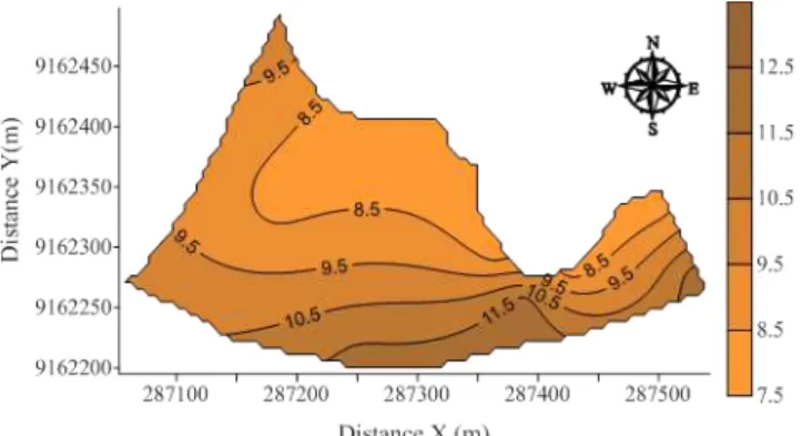
The experiment was carried out in an area of about 6.5 ha of the Santa Teresa sugar and alcohol industry, in Goiana, Zona da Mata Norte, State of Pernambuco, Brazil (07°34'25''S, 34°55'39''W and average altitude of 8.5 m) (Figure 1).
Figure 1. Topographic map of the study area.
The soil of the experimental area was classified as orthic Humiluvic Spodosol of sandy texture, according to the classification of EMBRAPA
The climate of the region is tropical humid type As', i.e., hot and humid, according to the classification of Köppen, with a rainy season from autumn to winter, annual average precipitation of 1,924 mm and annual average temperatures of 24 °C.
The study area has been used for rainfed sugarcane (Saccharum officinarum L.) crops, grown as single-crop, with straw burning before harvesting,
since 1988. The crop area had been renewed in the 2010-2011 crops season; the soil was plowed,
harrowed, grooved, limed, and fertilized and the
sugarcane variety RB867515 was planted.
Ninety sampling points were randomly chosen in the study area (Figure 2) and georeferenced with a GPS device with differential correction to subsequent data collection of the soil texture (clay, silt and sand), electrical conductivity of the saturation extract (ECse) and water content.
Samplings were carried out in January 21, 2014, with texture, ECse and water content determined in the soil
layers of 0.0-0.2 and 0.2 -0.4 m.
Table 1. Textural classification of an orthic Humiluvic Spodosol.
Layer (m) Texture (g kg
-1 )
Clay Silt Sand
0.0-0.2 253.20 33.91 712.89
0.2-0.4 253.38 26.87 719.76
Figure 2. Location of the sampling points in the study area.
Field evaluations of soil apparent electrical conductivity (ECa) (mS m-1) was carried out using an
electromagnetic induction device (EM38) (GEONICS, 1999), which measures the horizontal dipole (ECa-H), with readings within the soil layer
0.0-0.4 m and the vertical dipole (ECa-V), with
readings within the layer 0.0-1.5 m, following the
procedures described by Siqueira, Silva and Dafonte (2015) and Siqueira et al. (2016b).
Field evaluations of the volumetric water content in the soil (θ%) in the soil layers 0.0-0.2 and
0.2-0.4 m was carried out using a transmission line
oscillator (Hydrosense®, Campbell Scientific
Australia Pty. Ltd.), which has a probe that emits an electromagnetic signal in the soil and evaluates how many times the signal returns in a certain period of time (SIQUEIRA et al., 2015).
Laboratory evaluations of the soil texture (clay, silt and sand) (g kg-1) and EC
se (dS m-1) were
carried out in samples of the soil layers 0.0-0.2 and
0.2-0.4 m. The samples were air dried,
disaggregated, sieved in a 2 mm mesh sieve. Soil texture (g kg-1) was determined with a densimeter
and ECse by the saturated paste extract method,
following the procedures described by EMBRAPA (2011).
The means of the attributes were subjected to the main statistical procedures (mean, median, standard deviation, coefficient of variation, skewness and kurtosis). The normality of the data was evaluated through coefficients of skewness and kurtosis and histograms of frequency distribution. The coefficient of variation (CV, %) was classified as low (<12%), intermediate (12% to 62%) and high (>62%) (WARRICK; NIELSEN, 1980). The linear correlation between the attributes was determined with significance level of 1% using the Shapiro-Wilk
test, including the relief data of all sampling points to assess the effect of relief on the variables. Statistical analyzes were performed using software R 3.3.1 (R CORE TEAM, 2016).
Rev. Caatinga
semivariance γ(h), which is estimated by the Equation (1),
in which N (h) is the number of experimental pairs of observations Z (xi) and Z(xi + h) separated by the
distance h.
The semivariograms were developed according to VIEIRA (2000) in the software R. The spatial dependence index (SDI) was determined according to Cambardella et al. (1994), who classified dependences as strong (<25%), moderate (25 to 75%) and weak (>75%).
The software Surfer 11.0 was used to develop maps of spatial variability. Isoline maps were
𝛾 ℎ = 1
2𝑁(ℎ) 𝑍 𝑋𝑖 − 𝑍(𝑋𝑖+ℎ)
2 𝑁(ℎ)
𝑖=1
developed when the pure nugget effect was detected to compare the attributes, using the Surfer's default parameters, which is based on a linear interpolation model by kriging.
RESULTS AND DISCUSSION
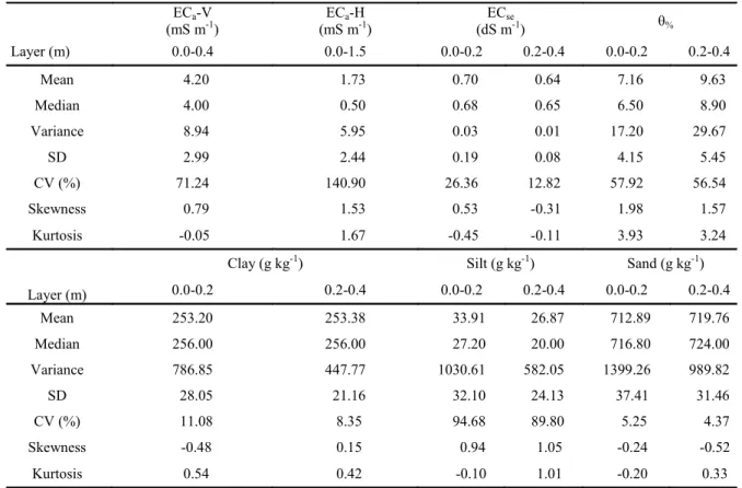
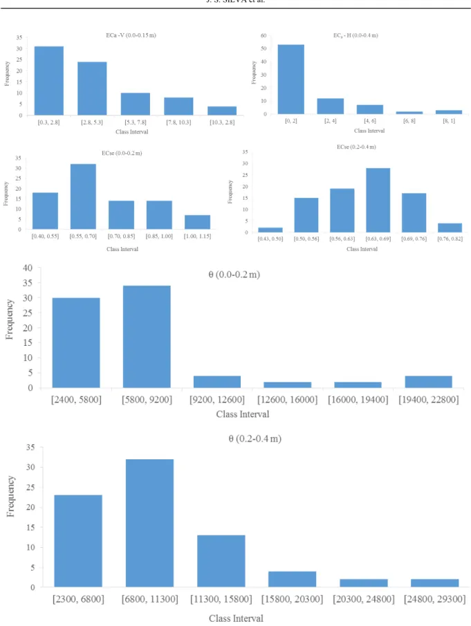
According to the mean and median analysis (Table 2), the data of all variables tended to normality. However, the analysis of frequency distribution graphs (Figures 3 and 4) showed different distributions (symmetrical and asymmetrical). The coefficients of skewness and kurtosis were different than 0 and 3, thus, the data did not show normal distribution.
ECa-V
(mS m-1)
ECa-H (mS m-1)
ECse
(dS m-1) θ%
Layer (m) 0.0-0.4 0.0-1.5 0.0-0.2 0.2-0.4 0.0-0.2 0.2-0.4
Mean 4.20 1.73 0.70 0.64 7.16 9.63
Median 4.00 0.50 0.68 0.65 6.50 8.90
Variance 8.94 5.95 0.03 0.01 17.20 29.67
SD 2.99 2.44 0.19 0.08 4.15 5.45
CV (%) 71.24 140.90 26.36 12.82 57.92 56.54
Skewness 0.79 1.53 0.53 -0.31 1.98 1.57
Kurtosis -0.05 1.67 -0.45 -0.11 3.93 3.24
Clay (g kg-1) Silt (g kg-1) Sand (g kg-1)
Layer (m) 0.0-0.2 0.2-0.4 0.0-0.2 0.2-0.4 0.0-0.2 0.2-0.4 Mean 253.20 253.38 33.91 26.87 712.89 719.76
Median 256.00 256.00 27.20 20.00 716.80 724.00
Variance 786.85 447.77 1030.61 582.05 1399.26 989.82
SD 28.05 21.16 32.10 24.13 37.41 31.46
CV (%) 11.08 8.35 94.68 89.80 5.25 4.37
Skewness -0.48 0.15 0.94 1.05 -0.24 -0.52
Kurtosis 0.54 0.42 -0.10 1.01 -0.20 0.33 Table 2. Descriptive statistics of attributes of an orthic Humiluvic Spodosol of sandy texture.
ECa-V = soil apparent electrical conductivity measured by electromagnetic induction with vertical dipole in the soil layer
Rev. Caatinga
The means of ECa-V and ECa-H were
different. According to Siqueira, Silva and Dafonte (2015) and Siqueira et al. (2016a), the largest differences in soil apparent electrical conductivity, measured by electromagnetic induction (ECa-V and
ECa-H) are due to soil relief, water rate fluctuation,
water content, texture and organic matter content. The water content in the soil and soil texture varied in both depths, explaining the greatest differences between ECa-V and ECa-H. Moreover, 80% of the
ECa-V readings were directly related to the ECa-H
readings, as also found by Geonics (1999) and Siqueira, Silva and Dafonte (2015). Therefore, despite the different means of ECa-V and ECa-H,
these variables are correlated.
ECa-V (mS m-1), ECa-H (dS m-1) and ECse
(dS m-1) means were different. However, despite
representing the same soil attribute, they were evaluated through different methods and expressed in different scales. Their major differences were due to evaluation method, since the electromagnetic induction method is assessed in the field, considering the soil electric current flow as a three-dimensional
body, encompassing a larger volume of soil (consisting of porous spaces, water and mineral particles), and ECse is determined in laboratory,
under controlled conditions, using disturbed soil samples, with readings that consider only the salts of the soil solution. (SIQUEIRA et al., 2014; SIQUEIRA; SILVA; DAFONTE, 2015).
The coefficient of variation (CV%) of clay and sand was classified as low (< 12%); water content in the soil (θ%) and ECse had intermediate
CV (12% to 62%); and ECa-V, ECa-H and silt
content had high CV (> 62%).
According to the frequency distribution histograms (Figure 3), most attributes had lognormal distribution, however, geostatistical analysis can be carried out despite the data normality (VIEIRA, 2000).
The frequency distribution graphs for ECa-V
and ECa-H showed leptokurtic positively skewed
distribution, i.e., there were many low ECa-V and
ECa-H, thus, their mode and median were close and
their means were overestimated. The ECse of the soil
layer 0.0-0.2 m also had leptokurtic positively
skewed distribution, whereas the ECse of the soil
layer 0.2-0.4 m had normal frequency distribution,
with slightly trend to a negatively skewed distribution. The histograms for ECa-V, ECa-H and
ECse was probably affected by the relief, as reported
by Siqueira, Silva and Dafonte (2015), who found the relief affecting the water flow in the soil and consequently, the ECa-V, ECa-H and ECse.
The water content in the soil (θ%) had
lognormal frequency distribution, also with overestimation of the mean and leptokurtic
positively skewed distribution. This result was expected, since the water flow and distribution in the soil favor the formation of sites with high and low water content as a function of relief, as reported by Siqueira et al. (2015). The frequency distribution histograms for water content in the soil showed very elongated tails, confirming that the water content varied, showing areas of high and low water content along the landscape of the study area.
Only the data of silt, from the texture attribute, had lognormal frequency distribution in both soil layers. Data of clay and sand had normal distribution, with more homogeneous histograms and less elongated tails, resulting in more stable means.
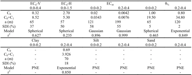
According to the geostatistical analysis (Table 3), most of the texture attributes had pure nugget effect (PNE), denoting a small scale spatial variability, i.e., at distances smaller than that chosen by random sampling. Only the model for clay content of the soil layer 0.2-0.4 m fitted to the
experimental semivariogram.
The spherical model was fitted to the semivariograms of ECa-V, ECa-H and θ (0.0-0.2);
and the Gaussian model to ECse in both layers. The
spherical model fit to the semivariograms for most of the attributes, confirming reports of other authors, who describe this model as that that best fit to the attributes of the soil (CAMBARDELLA et al., 1994; VIEIRA, 2000; SIQUEIRA; SILVA; DAFONTE, 2015; SIQUEIRA et al., 2016a).
The highest range (a) (m) was found for the ECse in the soil layer 0.2-0.4 m (199 m) and the
lowest, for the ECa-H in the soil layer 0.2-0.4 m
(57 m).
According to the classification of Cambardella et al. (1994), the attributes evaluated had strong (< 25%,) and moderate (25 to 75%) spatial dependence index. Siqueira et al. (2015) evaluated the spatial variability of soil attributes with different scales and found high SDI (%) for water
content in the soil (%) at different soil depths (0.0-0.2, 0.2-0. 4 and 0.4-0.6 m). Differences in
spatial dependence index were due to the soil natural variation and relief of the study area.
Parameters of models fitted to the experimental semivariogram of ECa-V and ECa-H
showed a similar spatial pattern, fitting a spherical model. The ECse spatial pattern was different,
especially by fitting a Gaussian mathematical model. This result was due to the scalar magnitude and because readings were performed in undisturbed (ECa-V and ECa-H) and disturbed (ECse) soil
samples.
According to the linear correlation matrix (Table 4), the relief was significantly correlated at 1% of probability (Shapiro-Wilk test) only to ECa-V
Rev. Caatinga
ECa-V ECa-H ECse θ%
0.0-0.4 0.0-1.5 0.0-0.2 0.2-0.4 0.0-0.2 0.2-0.4
C0 0.32 2.70 0.02 0.0042 1.00 0.80
C0+C1 8.52 5.30 0.0343 0.0076 19.50 34.80
a (m) 65 57 121 199 65 120 SDI (%) 37 50 58 55 5 2
Model Spherical Spherical Gaussian Gaussian Spherical Exponential r2 0.627 0.235 0.896 0.999 0.465 0.849
Clay Silt Sand
0.0-0.2 0.2-0.4 0.0-0.2 0.2-0.4 0.0-0.2 0.2-0.4
C0 - 0.69 - - - -
C0+C1 - 3.926 - - - -
a (m) - 70 - - - -
SDI (%) - 18 - - - -
Model PNE Exponential PNE PNE PNE PNE
r2 - 0.850 - - - -
Table 3. Parameters of models fitted to the experimental semivariogram of the attributes of an orthic Humiluvic Spodosol of sandy texture.
ECa-V = soil apparent electrical conductivity measured by electromagnetic induction with vertical dipole in the soil layer 0.0-0.4, ECa-H = soil apparent electrical conductivity measured by electromagnetic induction with horizontal dipole in the soil layer 0.0-1.5 m, ECse = electrical conductivity of the saturation extract, θ% = water content in the soil;
C0 = nugget effect, C0+C1 = sill, a = range (m), SDI: spatial dependence index (%), r2: coefficient of determination;
PNE = pure nugget effect.
The correlations of relief to ECes 0.0-0.2
(|r| = 0.337) and to ECse 0.2-0.4 (|r| = 0.051) were
low. This result was also due to the evaluation method used, with undisturbed (ECa-V and ECa-H)
and disturbed (ECse) soil samples.
Relief had no high linear correlation with the other attributes, since texture attributes are dependent on relief. Relief had some positive correlation only to silt (|r| = 0.419; 0.0-0.2) (|r| = 0.564; 0.2-0.4) and
sand (|r| = 0.559; 0.0-0.2) (|r| = 0.550; 0.2-0.4).
Relief ECa-V 0-1.5
ECa-H 0-0.4
ECse 0.0-0.2
ECse 0.2-0.4
θ 0.0-0.2
θ 0.2-0.4
Clay 0.0-0.2
Clay 0.2-0.4
Silt 0.0-0.2
Silt 0.2-0.4
Sand 0.0-0.2
Sand 0.2-0.4
Relief 1.000
ECa-V 0-1.5 0.815 1.000
ECa-H 0-0.4 0.826 0.940 1.000
ECse 0-0.2 0.337 0.530 0.638 1.000
ECse 0.2-0.4 0.051 0.350 0.543 0.564 1.000
θ 0-0.2 0.215 0.412 0.162 0.076 0.308 1.000
θ 0.2-0.4 0.374 0.531 0.464 0.338 0.249 0.497 1.000
Clay 0-0.2 0.201 0.254 0.572 0.197 0.583 0.611 0.295 1.000
Clay 0.2-0.4 0.185 0.284 0.486 0.394 0.686 0.527 0.231 0.510 1.000
Silt 0-0.2 0.419 0.533 0.642 0.230 0.679 0.343 0.219 0.611 0.304 1.000
Silt 0.2-0.4 0.564 0.640 0.599 0.582 0.717 0.290 0.430 0.477 0.300 0.377 1.000
Sand 0-0.2 0.559 0.665 0.304 0.245 0.428 0.703 0.416 0.675 0.451 0.407 0.460 1.000
Sand 0.2-0.4 0.550 0.907 0.227 0.397 0.444 0.493 0.570 0.953 0.913 0.739 0.198 0.678 1.000
Table 4. Linear correlation matrix for the attributes of an orthic Humiluvic Spodosol of sandy texture.
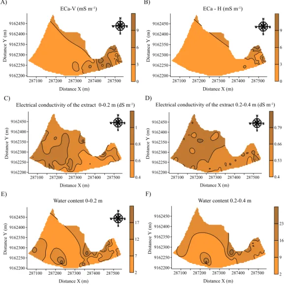
According to the spatial variability maps (Figures 5 and 6), the ECa-V (Figure 5A) and ECa-H
(Figure 5B) had similar distribution of the contour lines, explaining their high correlation (|r| = 0.940). Moreover, the device used reads a same volume of soil, and vertical dipole readings (ECa-V) are
affected by the soil surface layer, which was evaluated by the horizontal dipole (ECa-V)
(CORWIN; LESCH, 2003, 2005; SIQUEIRA; SILVA; DAFONTE, 2015).
The spatial variability maps of ECa-V, ECa-H,
ECse and θ showed no similar patterns (Figure 5),
confirming their low spatial correlation (Table 4). However, these maps followed a same trend pattern, as shown in the relief map (Figure 1). Therefore, the spatial distribution of the attributes (ECa-V, ECa-H,
ECse and θ) is affected by relief. According to
Siqueira, Silva and Dafonte (2015) and Siqueira et al. (2015), soil declivity is the factor that most affect water distribution and consequently, the distribution and interaction of other soil attributes.
The maps of water content in the soil (θ) at 0.0-0.2 (Figure 5E) and 0.2-0.4 m (Figure 5F)
showed the greatest similarity to the relief map (Figure 1) regarding the pattern of contour lines, however, with low correlation (|r| = 0.215; 0.0-0.2)
(| r | = 0.374; 0.2-0.4).
Spatial variability maps of texture (clay, silt and sand) (Figure 6) in the soil layers 0.0-0.2 and
0.2-0.4 m (Figure 6) showed no spatial relationship
with the maps of ECa-V, ECa-H, ECse and θ
(Figure 5), confirmed by the low values of linear correlation (Table 4).
The spatial distribution maps of soil texture (clay, silt and sand) showed great difference in contour lines, denoting high spatial variability. All texture attributes had pure nugget effect (PNE), except the clay at 0.2-0.4 m (Table 3). These maps
were developed by linear interpolation to compare spatial patterns, even with PNE, since cartography is a classical science, and data with PNE processed by geostatistics are usually not properly analyzed. Thus, the PNE of texture attributes was due to the high variability of the data along the landscape, affected by different soil formation factors (SIQUEIRA; SILVA; DAFONTE, 2015; SIQUEIRA et al., 2015).
A) B)
C) D)
E) F)
Rev. Caatinga
A) B)
C) D)
E) F)
Figure 6. Isoline maps of soil texture (clay, silt and sand) in the soil layers 0.0-0.2 m and 0.2-0.4 m of an orthic Humiluvic Spodosol of sandy texture.
CONCLUSIONS
Spatial variability of the soil apparent electrical conductivity measured by electromagnetic induction (ECa-V and ECa-H) was affected by relief
and had no direct correlation to the electrical conductivity of the soil saturation extract (ECse).
The soil attributes evaluated had frequency of distribution with overestimated means, and means distant from the mode and median.
The area relief affected the spatial variability of ECa-V, ECa-H, ECse and θ, however, the
correlation matrix did not show a well-defined cause
-and-effect relationship.
Spatial variability of soil texture attributes (clay, site and sand) was high, presenting pure nugget effect.
ACKNOWLEDGMENTS
The authors would like to thank CAPES
(Coordenação de Aperfeiçoamento de Pessoal de
Nível Superior, Brazil), CNPq (Conselho Nacional de Desenvolvimento Científico e Tecnológico, Brazil), FACEPE (Fundação de Amparo à Ciência e Tecnologia de Pernambuco, Brazil) and FAPEMA
(Fundação de Amparo à Pesquisa e ao
Desenvolvimento Científico e Tecnológico do Maranhão, Brazil) for financial support for excecution of the project and publication of the article.
REFERENCES
Comparing bulk soil electrical conductivity determination using the DUALEM-1S and EM38
-DD electromagnetic induction instruments. Soil Science Society of American Journal, Madison, v. 71, n. 1, p. 189-196, 2007.
ALVES, S. M. et al. Definição de zonas de manejo a partir de mapas de condutividade elétrica e matéria orgânica. Bioscience Journal, Uberlândia, v. 29, n. 1, p. 104-114, 2013.
AMEZKETA, E. Soil salinity assessment using directed soil sampling from a geophysical survey with electromagnetic technology: a case study.
Spanish Journal Agricultural Research, Madrid, v. 5, n. 1, p. 91-101, 2007.
ATWELL, M. A.; WUDDIVIRA, M. N.; GOBIN, J. F. Abiotic water quality control on mangrove distribution in estuarine river channels assessed by a novel boat-mounted electromagnetic-induction
technique. Water SA, Pretoria, v. 42, n. 3, p. 399
-407, 2016.
BREVIK, E. C. Analysis of the representation of soil map units using a common apparent electrical conductivity sampling design for the mapping of soil properties. Soil Survey Horizons, Madison, v. 53, n. 2, p. 32-37, 2012.
CAMBARDELLA, C. A. et al. Field-scale
variability of soil proprieties in central Iowa soils.
Soil Science Society America Journal, Madison, v. 58, n. 5, p. 1240-1248, 1994.
CORWIN, D. L.; LESCH, S. M. Application of soil electrical conductivity to precision agriculture: theory, principles, and guidelines. Agronomy Journal, Madison, v. 95, n. 3, p. 455-471, 2003.
CORWIN, D. L.; LESCH, S. M. Apparent soil electrical conductivity measurements in agriculture.
Computers and Electronics in Agriculture, Amsterdam, v. 46, n. 1-3, p. 11-43, 2005.
EMPRESA BRASILEIRA DE PESQUISA AGROPECUÁRIA - EMBRAPA. Manual de métodos de análise do solo. 2. ed. Rio de Janeiro,
RJ: Embrapa Solos, 2011, 212 p.
EMPRESA BRASILEIRA DE PESQUISA AGROPECUÁRIA - EMBRAPA. Sistema brasileiro de classificação de solos. 3. ed. Rio de
Janeiro, RJ: Embrapa Solos, 2013. 353 p.
FITZGERALD, G. J. et al. Directed sampling using remote sensing with a response surface sampling design for site-specific agriculture. Computers and Electronics in Agriculture, Amsterdam, v. 53, n. 2, p. 98-112, 2006.
GEONICS, EM 38. Ground conductivity meter operating manual. Ontário: Geonics Ltda. 1999. 69 p.
GUO, W.; MAAS, S. J.; BRONSON, K. F. Relationship between cotton yield and soil electrical conductivity, topography and landsat imagery.
Precision Agriculture, Dordrecht, v. 13, n. 6, p. 678
-692. 2012.
KÜHN, J. et al. Interpretation of electrical conductivity patterns by soil properties and geological maps for precision agriculture. Precision Agriculture, Dordrecht, v. 10, n. 6, p. 490-507,
2009.
MOLIN, J. P.; RABELLO, L. M. Estudos sobre mensuração da condutividade elétrica do solo.
Engenharia Agrícola, Jaboticabal, v. 31, n. 1, p. 90 -101, 2011.
R CORE TEAM. R: A language and environment for statistical computing. R Foundation for
Statistical Computing, Vienna, Austria. 2016. Disponível em:<http://www.rprojetc.org.>. Acesso em: 20 dez. 2016.
SHANER, D. L.; FARAHANI, H. J.; BUCHLEITER, G. W. Predicting and Mapping Herbicide-Soil Partition Coefficients for EPTC,
Metribuzin, and Metolachlor on Three Colorado Fields. Weed Science, Champaign, v. 56, n. 1, p. 133–139, 2008.
SILVA, J. S. et al. Distribuição espacial da condutividade elétrica e matéria orgânica em Neossolo Flúvico. Revista Brasileira de Geografia Física, Recife, v. 6, n. 4, p. 764-776, 2013.
SIQUEIRA, G. M.; SILVA, E. F. F.; DAFONTE, J. D. Distribuição espacial da condutividade elétrica do solo medida por indução eletromagnética e da produtividade de cana-de-açúcar. Bragantia,
Campinas, v. 74, n. 2, p. 215-223, 2015.
SIQUEIRA, G. M. et al. Using Multivariate Geostatistics to Assess Patterns of Spatial Dependence of Apparent Soil Electrical Conductivity and Selected Soil Properties. The Scientific World Journal, New Work, v. 2014, n. 1, p. 1-11, 2014.
SIQUEIRA, G. M. et al. Estacionariedade do conteúdo de água de um Espodossolo Humilúvico.
Revista Brasileira de Engenharia Agrícola e Ambiental, Campina Grande, v. 19, n. 5, p. 439-448,
2015.
Rev. Caatinga
electromagnetic induction. African Journal of Agricultural Research, Nairobi, v. 11, n. 39, p. 3751-3762, 2016a.
SIQUEIRA, G. M. et al. Spatial soil sampling design using apparent soil electrical conductivity measurements. Bragantia, Campinas, v. 75, n. 4, p. 459-473, 2016b.
VIEIRA, S. R. Geoestatística em estudos de variabilidade espacial do solo. In: NOVAIS, R. F.; ALVAREZ VENEGAS, V. H.; SCHAEFER, G. R.
(Eds.). Tópicos em Ciência do solo. Viçosa:
Sociedade Brasileira de Ciência do Solo, 2000. v. 1, cap. 6, p. 1-54.
WARRICK, A. W.; NIELSEN, D. R. Spatial variability of soil physical properties in the field. In: HILLEL, D. (Ed.). Applications of soil physics. New York: Academic Press, 1980. cap. 2, p. 314
-344.