Soil and Plant Nutrition /Article
Spatial distribution of soil apparent electrical
conductivity measured by electromagnetic induction
and sugarcane yield
Glécio Machado Siqueira (1*); Ênio Farias de Franca e Silva (2); Jorge Dafonte Dafonte (3)
(1) Universidade Federal do Maranhão (UFMA), Centro de Ciências Agrárias e Ambientais, BR-222, km 04, s/n, 65500-000
Chapadinha (MA), Brasil.
(2) Universidade Federal Rural de Pernambuco (UFRPE), Departamento de Engenharia Agrícola, Rua Dom Manoel de Medeiros, s/n,
52171-900 Recife (PE), Brasil.
(3) Universidade de Santiago de Compostela (USC), Departamento de Engenharia Rural, Lugo, Galicia, Spain.
(*) Corresponding author: [email protected]
Received: July 23, 2014; Accepted: Dec. 18, 2014
Abstract
The current agriculture requires the use of new technologies that allow the identification of soil and plant patterns, and the determination of their spatial variability. This work determined the spatial relationship between the sugar cane yield and soil apparent electrical conductivity (ECa) measured by electromagnetic induction (EMI) and soil texture. The experimental area is located in Goiana (Pernambuco State, Brazil) (07°34’25”S, 34°55’39”W). The experimental area was 6.5 ha. Sugar cane yield and soil apparent electrical conductivity (ECa) were measured at 90 sampling points randomly distributed in the study area. Maps of soil electrical conductivity (ECa-V and ECa-H) were similar to that of sugar cane yield. The linear correlation showed values of 0.74 (yield x ECa-H) and 0.85 (yield x ECa-V). The electrical conductivity measured by electromagnetic induction has been shown to be an important tool for predicting the yield of sugar cane. The textural properties (clay, silt and sand) showed high spatial variability.
Key words: geostatistics, precision agriculture, soil management zones.
1. INTRODUCTION
The agroindustrial complex of sugar cane, especially the alcohol production chain, places Brazil in the leading position in technological advance in the energy area from biofuel. In a global market with large and rapid flow of knowledge, maintaining competitiveness depends on an ongoing search for innovative technologies.
The National Supply Company (CONAB, 2012) provides for the 2012/2013 harvest an estimated planting area of 8,520.5 billion hectares, distributed in all producing states, representing an increase of 2.0% over the previous season. The average yield of the 2012/2013 harvest was 69.44 t ha–1 and a production of
595.13 million tons (CONAB, 2012). The Pernambuco State, according to CONAB (2012), has an area planted with sugar cane of 327.61 thousand hectares in the 2012/2013 season, with a yield of 45.5 t ha–1, and a
production 14,906.3 million tons.
The increased production of sugar cane creates the need to assess the economic, social and environmental
impacts of this process, both for the country as a whole and for the producing regions. Thus, the current agriculture needs methodologies to promote changes in the technique for quantification of soil attributes in order to assist the characterization of the variability of these attributes rapidly and accurately (Siqueira et al., 2010). However, the costs involved, the high demand for time and labor and the need for human resources with high technical potential make unworkable the implementation of these detailed studies using numerical classification (Figueiredo et al., 2008).
as site specific management zones. According to these authors, the identification of these specific management zones allows the application of technology to similar areas.
These compartments have been used for different purposes in soil science: sampling design (Montanari et al., 2005); dynamics of clay mineral formation (Camargo et al., 2008.); nutrient adsorption potential (Barbieri et al., 2008); soil loss (Campos et al., 2008); input application at varying rates (Barbieri et al., 2009); agricultural planning and implementation of sugar cane farming system (Campos et al., 2009), CO2 emission (Brito et al., 2009), among others.
Among soil properties, the apparent electrical conductivity (ECa) has been widely used due to its correlation with other soil properties and therefore with yield of crops (Lesch et al., 2005; Siqueira et al., 2009, 2013). According to McNeill (1980), Lesch et al. (2005), Sudduth et al. (2005), Kühn et al. (2009) and Siqueira et al. (2009), ECa is related to the water content in the soil, texture, organic matter content, size and distribution of pores, salinity, cation exchange capacity and electrolyte concentration in the soil solution.
In this way, this study aimed to determine the spatial relationship between the sugar cane yield and the electrical conductivity of soil measured by electromagnetic induction and soil texture in a commercial production area under monoculture over 27 years, in Goiana, Pernambuco State, Brazil.
2. MATERIAL AND METHODS
The experimental area is located in the municipality of Goiana (Northern Zona da Mata, Pernambuco State, Brazil) at the coordinates 07°34’25”S latitude and 34°55’39”W longitude. The soils of the study region derive from the group Barreiras, consisting of sediments of continental origin of the late tertiary, texture sandy to clay, characterized by intense change (Brasil, 1969, 1972). Soil was classified as an OrthicPodzol (Soil Survey Staff, 2010), which is equivalent to an “Espodossolo Humilúvicoortico” following the Brazilian Soil Classification System (EMBRAPA, 2013), whose physical characterization is shown in table 1. Soil
texture (clay, silt and sand) was determined by the pipette method; bulk density and volumetric soil moisture were determined in the pedological profile using soil cores of 100 cm3 as proposed by Camargo et al. (1986).
The climate, according to the Köppen Climate Classification, is humid tropical type As’ or pseudo tropical, which is hot and humid, with rainfall in the fall and winter, with average annual temperatures around 24°C.
The study area is approximately 6.5 ha, at an average altitude of 8.5 m (Figure 1) and has been managed in the last 27 years with monoculture of sugarcane (Saccharum officinarum L.) with straw burning for harvesting. In the 2010/2011 growing season, the area was cleared, plowed, harrowed, and then grown again with sugar cane.
Sampling of sugar cane yield and the apparent soil electrical conductivity and texture was held on November 11st, 2011 at 90 sampling points in an uneven grid (Figure 2).
The study area is very important for the region, as the sugar cane is the main crop, located often in areas affected by salinity due to its proximity to the sea, especially in high tide periods, with more pronounced salinity in the lower sections. The area is located at about 10 km from the Atlantic Ocean on the east and 2.5 km to the northeast
Table 1. Physical propertie sof the OrthicPodzol
Layer (m)
--- Texture (g kg–1) --- Bulk density (kg dm–3)
Soilmoisture (m3 m–3) Clay Silt Sand
0.0-0.3 44 26 930 1.52 0.345
0.3-0.60 43 25 932 1.54 0.368
0.6-1 44 26 930 1.60 0.426
> 1 m 32 40 928 1.66 0.472
Figure 1. Topographic map of the study area.
from a river that flows into the ocean, suffering saline influence from two different sources.
Sugar cane yield was determined by the method proposed by Gheller et al. (1999), which estimates the total weight of the plot by multiplying the number of stems of the sampled area by the average weight of ten stems. At each sampling point, we chose three rows of sugar cane ten meters long, and counted the number of stems for calculating their average weight. Subsequently, ten stems were harvested at random among the three rows of each sampling point for weighing.
Thus, yield can be calculated as follows, as described by Gheller et al. (1999):
a) Average weight per stem:
ms Aps
tstems
= (1)
where: msis the weight of the bundle with 10 stems; Tstems
is the total of stems counted in the three rows.
b) Weight estimated at the sampling point:
Aps Yield
Tstems
= (2)
With the average weight estimated in each sampling point, we can calculate the yield per hectare (t ha–1).
The apparent soil electrical conductivity (ECa, mS m–1)
was measured by electromagnetic induction with the equipment EM38 (Geonics) at two depths: vertical dipole (effective depth of 1.5 m - ECa-V) and horizontal dipole (effective depth of 0.4 m - ECa-H). Values of ECa measured in the field (ECa-V and ECa-H) were then correlated with soil temperature, according to Huth & Poulton (2007). However, as it is a small area where it is possible to measure the ECa in a short time, the corrections of ECa values by soil temperature provided no consistent change in the original values, so we used the original values of ECa.
Soil texture (clay, silt and sand) was determined at the layers 0.0-0.2 m and 0.2-0.4 m deep, according to Camargo et al. (1986).
The statistical parameters (mean, standard deviation, coefficient of variation, skewness and kurtosis) were determined for each sampling point. Coefficients of variation (CV, %) were used to determine the variability of the data, according to the classification Warrick & Nielsen (1980).
For the analysis of spatial variability, data were analyzed using geostatistical methods of semivariogram analysis, described by Vieira (2000), and based on the assumptions of stationarity of the intrinsic hypothesis. The spatial correlation between neighboring sites was calculated
using the semi-variance γ(h), with the aid of the software GEOSTAT (Vieira et al., 2002).
Mathematical models were fitted to the semivariogram, which allowed the analysis of the spatial variation of variables. Criteria and procedures for semivariogram model fit were performed according to Vieira (2000), considering the methods of ordinary least squares and weighted least squares and cross-validation. From the fit of a mathematical model to the data, the semivariogram parameters were defined:
a) nugget effect (C0), which is the value of γ when h = 0;
b) range of spatial dependence(a), which is the distance in whichγ(h) remains approximately constant, after increasing with the increase of h;
c) sill (C0+C1), which is the value of γ(h) from the range, which approximates the variance of the data, if any.
The preliminary geostatistical analysis indicated a trend in the data of sugar cane yield (t ha–1), which was
removed through the following equations for estimation of residuals:
1. Linear
0 1 2 3
m( x )=A +A x+A y+A xy (3)
2. Quadraticorparabolic
2 2
0 1 2 3 4 5
m( x )=A +A x+A y+A x +A y +A xy (4)
3. Cubic
2 2
0 1 2 3 4
3 3 2 2
5 6 7 8 9
m( x ) A A x A y A x A y
A xy A x A y A x y A xy
= + + + + +
+ + + + (5)
The scaled semivariogram was constructed with the purpose of evaluating the spatial variability patterns between studied attributes (Vieira, 2000; Vieira et al 2002).
The analysis of the spatial dependence degree (SSD) of variables used the classification of Cambardella et al. (1994) considering the following relationship: (C0/C0+C1)*100, in which 0 to 25% (strong), between 25 and 75% (moderate) and>75% (poor).
SURFER, which is based on a linear kriging interpolation (Golden Software Inc., 1999).
3. RESULTS AND DISCUSSION
The average yield of sugar cane in the study area was75.54 t ha–1 (Table 2). The yield in the area is about
66.02% higher compared to the average of the Pernambuco State for the growing season of 2012/2013 (CONAB, 2012). Domestic production in the 2012/2013 season (CONAB, 2012) was 69.44 t ha–1, with a yield in the
area 8.78% higher than the national average.
Mean values for the apparent soil electrical conductivity measured by electromagnetic induction in the vertical (ECa-V) and horizontal (ECa-H) dipoles were relatively similar (Table 2). This is probably because, at the time of sampling, the water table was close to the surface (Siqueira et al., 2013), which is the factor that interfered most with the readings taken with the EM38, corroborating Lesch et al. (2005). At the lower sections of the area, the water table was 0.2 m above the ground surface, moving away from the surface with increasing topography.
The yield showed the greatest variance of the data, since it varies considerably with soil changes across the landscape Coefficients of variation (CV, %) were classified as median (12-60%), according to Warrick & Nielsen (1980). There was an increase in CV values for ECa-V (31.10%) and ECa-H (40.60%). Siqueira et al. (2009) reports that the major differences in electrical conductivity measured by electromagnetic induction between the surface and the depth layers should be due to greater differences in water content in the surface layer, because in deep layers, such content becomes more stable. Confirmed by the analysis of the topographic map (Figure 1), since at the time of sampling the lower sections of the area were soaked, while at the higher sections, the water table was
more away from the surface, explaining the differences in ECa readings.
The textural properties (clay, silt and sand - g kg–1)
confirmed the sandy texture of the study area in the two studied layers (0.0-0.2 and 0.2-0.4 m), however the average of sand content (Table 2) found on the surface layer (0.0-0.2 m) and at the subsurface layer (0.2-0.4 m) was about 20% lower than the representative profile for the study area (Table 1). The coefficients of variation (CV, %) were low for all textural properties. This fact is related to the process of soil formation in the study area, which is based on sedimentation, making the finer particles to deposit in depth and the coarsest particles in the upper layer (Brazil, 1969, 1972).
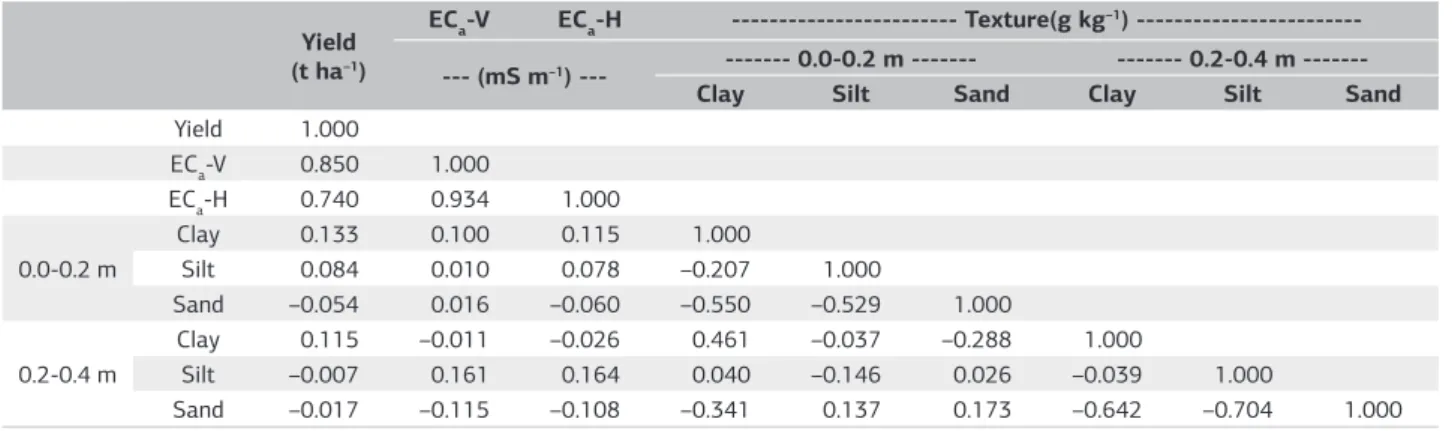
The linear correlation between the properties (Table 3) showed the highest value between ECa-V x ECa-H (0.934). This high correlation is due to the nature of measuring both properties, since according to Lesch et al. (2005), up to 80% of the response obtained with the vertical dipole (ECa-V) originates from the soil surface layer (ECa-H). The linear correlation between yield and ECa was high, with values of 0.850 (yieldx ECa-V) and 0.740 (yield x ECa-H).
Dantas et al. (2006) reported increased yield of sugar cane when there is no water deficit. In this way, high correlations between yield x ECa-V (0.850) and yield xECa-V(0.740) are expected, since in higher areas, the yield is lower and hence ECa values, thus increase in yield an din ECa values are found in the lower sections of the area.
However, when correlating sugar cane yield with the content of clay, silt and sand in the layers of 0.0-0.2 m and 0.2-0.4 m (Table 3), the correlation values were low or zero, according to the classification proposed by Santos (2007). The same is true for the correlation between the textural properties and ECa-V and ECa-H. The occurrence of low linear correlation values between the textural properties and ECa-V and ECa-Hwas not expected, as the soil clay content is the property that interferes most
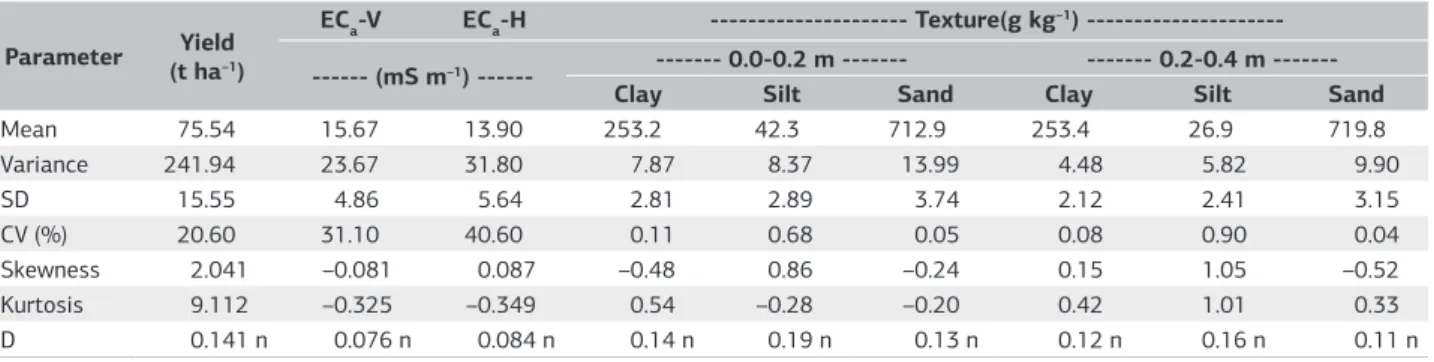
Table 2. Statistical parameters for the sugar cane yield (t ha–1), the electrical conductivity of soil measured by electromagnetic induction
(ECa-V and ECa-H, mS m–1) and soil texture (g kg–1)
Parameter Yield (t ha–1)
ECa-V ECa-H --- Texture(g kg–1) --- (mS m–1) --- --- 0.0-0.2 m --- 0.2-0.4 m
---Clay Silt Sand Clay Silt Sand
Mean 75.54 15.67 13.90 253.2 42.3 712.9 253.4 26.9 719.8
Variance 241.94 23.67 31.80 7.87 8.37 13.99 4.48 5.82 9.90
SD 15.55 4.86 5.64 2.81 2.89 3.74 2.12 2.41 3.15
CV (%) 20.60 31.10 40.60 0.11 0.68 0.05 0.08 0.90 0.04
Skewness 2.041 –0.081 0.087 –0.48 0.86 –0.24 0.15 1.05 –0.52
Kurtosis 9.112 –0.325 –0.349 0.54 –0.28 –0.20 0.42 1.01 0.33
D 0.141 n 0.076 n 0.084 n 0.14 n 0.19 n 0.13 n 0.12 n 0.16 n 0.11 n
with the values of ECa-V and ECa-H (McNeill, 1980; Lesch et al., 2005; Sudduth et al., 2005; Kühn et al., 2009; Siqueira et al., 2009). This fact is related to water surplus in the study area, represented by the water table very close to the surface at the time of harvesting sugar cane and sampling other soil properties under study.
Negative linear correlation values between the textural properties were expected, since with the increase in sand content in the study area there is a reduction in the amount of clay and silt, with the highest correlation found for the silt × sand at the layer 0.2-0.4 m (–0.704).
The geostatistical analysis (Table 4) showed that the Gaussian model was the best fit to the data set. Siqueira et al. (2009) studied the spatial variability of soil electrical conductivity in area with topographic gradient and fitted the spherical model to ECa at the surface and depth layers. The fit of the Gaussian model to the data (Table 4) may be associated with the concave relief in the study area, coinciding with the areas with higher yields and consequently with higher ECa values due to the greater water content in the soil when compared the higher sections of the area. Data of sugar cane yield presented a trend and we calculated the residuals through a linear equation. Siqueira et al. (2010) demonstrate how the geomorphology of the soil interferes with the identification of specific management zones, with the fit of different semivariograms
for each of the management zones. Different authors have justified the importance of soil geomorphology for sampling design (Montanari et al., 2005); dynamics of clay mineral (Camargo et al., 2008); nutrient adsorption potential (Barbieri et al., 2008); soil loss (Campos et al., 2008); input application at varying rates (Barbieri et al., 2009); agricultural planning and implementation of sugar cane farming system (Campos et al., 2009), CO2 emissions (Brito et al., 2009), among othes.
The yield showed a range (a, m) of 110.00 m while ECa-V and ECa-H showed a value of 180.00 m (Table 4). This is because, among the plant attributes, yield is the most sensitive to soil changes. The spatial dependence was determined as proposed by Cambardella et al. (1994), indicating high correlation between samples (SSD ≤ 25.00%).
The scaled semivariograma showed the existence of a similar pattern of spatial variation between yield and ECa-V and ECa-H (Table 4). However, the pattern occurs at different levels of spatial variability, since the yiel dreaches higher values of C0and C1, related to the higher variation in yield values across the area (variance = 241.94) when compared to ECa-V (23.67) and ECa-H (31.80, Table 2).
Additionally, the scaled semivariogram was modeled to check for a similar spatial pattern between semivariance pairs for yield, and the ECa-V and the ECa-H (Figure 3).
Table 3. Linear correlation between sugar cane yield (t ha–1), soil electrical conductivity measured by electromagnetic induction (EC a-V
andECa-H,mS m–1) and soil texture (g kg–1)
Yield (t ha–1)
ECa-V ECa-H --- Texture(g kg–1) --- (mS m–1) --- --- 0.0-0.2 m --- 0.2-0.4 m
---Clay Silt Sand Clay Silt Sand
Yield 1.000
ECa-V 0.850 1.000
ECa-H 0.740 0.934 1.000 0.0-0.2 m
Clay 0.133 0.100 0.115 1.000
Silt 0.084 0.010 0.078 –0.207 1.000
Sand –0.054 0.016 –0.060 –0.550 –0.529 1.000 0.2-0.4 m
Clay 0.115 –0.011 –0.026 0.461 –0.037 –0.288 1.000
Silt –0.007 0.161 0.164 0.040 –0.146 0.026 –0.039 1.000
Sand –0.017 –0.115 –0.108 –0.341 0.137 0.173 –0.642 –0.704 1.000
Table 4. Semivariogramfitting parameters for the yield of sugar cane (t ha–1), electrical conductivity of soil measured by electromagnetic
induction (ECa-V and ECa-H, mS m–1) and soil texture (g kg–1)
Residuals Yield (t ha–1)
ECa-V ECa-H --- Textura (g kg–1) --- (mS m–1) --- --- 0.0-0.2 m --- 0.2-0.4 m
---Clay Silt Sand Clay Silt Sand
Model Gaussian Gaussian Gaussian
PNE PNE PNE
Exponential
PNE PNE
C0 200 6 10 0.690
C0+C1 580 28 35 3.926
a (m) 110 180 180 70.00
SD 25.64 17.64 22.22 14.94
The values of ECa-V and ECa-H show similar behavior for the pairs of semivariance, while the pairs of semi-variance of soil yield (residuals) present a completely different behavior from ECa-V and ECa-H. As already discussed, this is due to the geomorphology of the area and the presence of higher moisture values in the lower sections of the landscape.
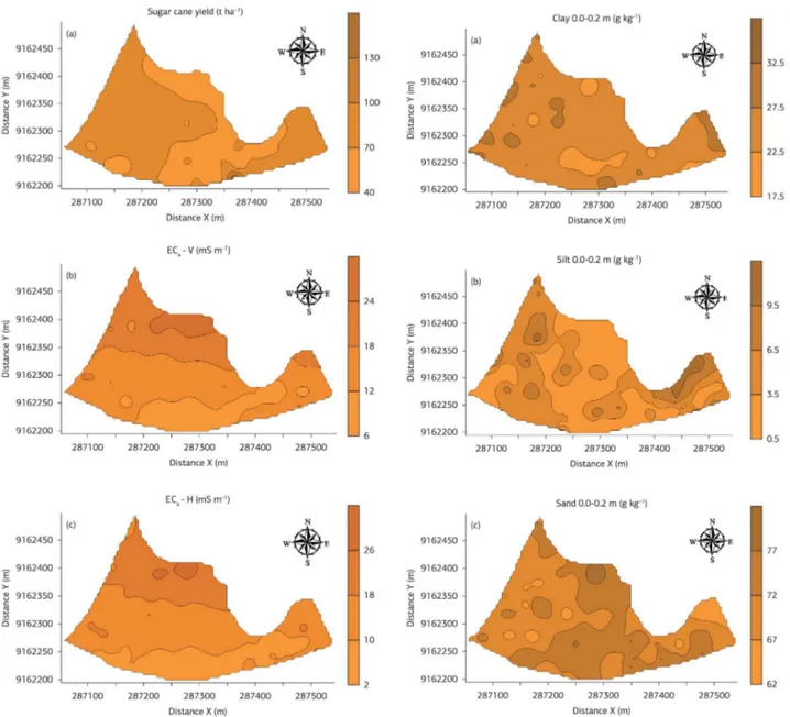
Maps of spatial variability confirm the similarity in the spatial distribution pattern for ECa-V and ECa-H (Figures 4a,b). As previously shown, this similarity is due to the higher values of soil moisture in the lower sections of the landscape, which, in turn favor a higher yield (Figure 4a). The greatest similarity between the analyzed properties occurs for thematic maps of ECa (Figures 4b,c).
Figure 4. Thematic maps of spatial variability for: a) yield (t ha–1);
b) ECa-V (mS m–1); c) EC
a-H (mS m –1).
Figure 5. Thematic maps of spatial variability for soil texture at the 0.0-0.2 m depth layer: a) clay (g kg–1); b) silt (g kg–1); c) sand (g kg–1). Figure 3. Scaled semivariogram for sugar cane yield (t ha–1) and
apparent soil electrical conductivity (ECa-V andECa-H, mS m–1)
The yield of sugar cane showed high linear correlation with ECa (Table 3), however, when analyzing the spatial variability maps (Figure 4), it is not possible to detect a clear relationship between the yield map (Figure 4a) and maps of ECa (Figures 4b,c). The yield map (Figure 4a) shows, in most of the area, yield values greater than 75.54 t ha–1, which represents the average yield of the
area, reaching values of up to 160 t ha–1, coinciding
with concave zone and with higher values of moisture when compared to other zones, corroborating once again the relationship between water of the crop and its yield (Dantas et al., 2006).
Moreover, the lower yield values are situated in the part where the area has smaller width (Figure 4a) and
its highest topographic elevation (Figure 1). Lower yield values were also registered also at the top left of the map, where the lowest topographic elevation is found, showing that excess moisture also influences the yield of sugar cane.
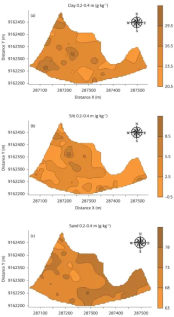
Maps of spatial variability of textural attributes (clay, silt and sand) at the 0.0-0.2 m layer (Figure 5) and 0.2-0.4 m layer (Figure 6) confirm that there is no relationship between maps of yield and ECa-V and ECa-H (Figure 4), corroborating the low linear correlation values shown in table 3. In general, maps of spatial variability of soil texture (Figures 5 and 6) indicated no similarity pattern in the arrangement of the contour lines of the textural classes. Nevertheless, in depth (Figure 6, 0.2-0.4m depth layer), there was an inverse relationship between the values of clay and sand (r = -0.642, Table 3) and between silt and sand (r = –0.704, Table 3).
4. CONCLUSION
The spatial variability maps present similar pattern for sugar cane yield and ECa-V and ECa-H. The electrical conductivity measured by electromagnetic induction has been shown to be an important tool for predicting the yield of sugar cane. The textural properties (clay, silt and sand) showed high spatial variability, demonstrating that the sampling design was not sufficient to determine the spatial distribution, whereas the relief and the water table are the factors that interfere most with the variability of all studied properties.
REFERENCES
Barbieri, D. M., Marques, J., Jr., & Pereira, G. T. (2008). Variabilidade espacial de atributos químicos de um argissolo para aplicação de insumos à taxa variável em diferentes formas de relevo. Engenharia Agrícola, 28, 645-653. http://dx.doi.org/10.1590/ S0100-69162008000400004.
Barbieri, D. M., Marques, J., Jr., Alleoni, L. F. R., Garbuio, F. J., & Camargo, L. A. (2009). Hillslope curvature, clay mineralogy, and phosphorus adsorption in an Alfisol cultivated with sugarcane. Scientia Agricola, 66, 819-826. http://dx.doi.org/10.1590/S0103-90162009000600015.
Brasil. Ministério da Agricultura. Departamento Nacional de Pesquisa Agropecuária. Divisão de Pesquisa Pedológica (1972). Levantamento exploratório-reconhecimento de solos do Estado de Pernambuco (Boletim Técnico, 26, Série Pedologia, 14). Recife: Convênio de mapeamento de solos MA/DNPEA-SUDENE/DRN convênio MA/CONTAP/USAID/ETA.
Brasil. Ministério da Agricultura. Escritório de Pesquisas e Experimentação. Equipe de Pedologia e Fertilidade do Solo (1969).
Levantamento detalhado dos solos da Estação Experimental de Itapirema (Boletim Técnico, 12). Rio de Janeiro. 84 p.
Brito, L. F., Marques, J., Jr., Pereira, G. T., Souza, Z. M., & La Scala, N., Jr. (2009). Soil CO2 emission of sugarcane fields as affected by topography. Scientia Agricola, 66, 77-83. http://dx.doi.org/10.1590/ S0103-90162009000100011.
Camargo, L. A., Marques, J., Jr., Pereira, G. T., & Horvat, R. A. (2008). Variabilidade espacial de atributos mineralógicos de um Latossolo sob diferentes formas de relevo. I-Mineralogia da fração argila. Revista Brasileira de Ciencia do Solo, 32, 2269-2277. http:// dx.doi.org/10.1590/S0100-06832008000600006.
Camargo, O. A., Moniz, A. C., Jorge, J. A., & Valadares, J. M. A. S. (1986). Métodos de análise química, mineralógica e física de solos do Instituto Agronômico de Campinas (Boletim técnico, 106). Campinas: Instituto Agronômico. 94 p.
Cambardella, C. A., Mooman, T. B., Novak, J. M., Parkin, T. B., Karlen, D. L., Turco, R. F., & Konopa, A. E. (1994). Field scale variability of soil properties in central Iowa soil. Soil Science Society of America Journal, 58, 1501-1511. http://dx.doi.org/10.2136/ss saj1994.03615995005800050033x.
Campos, M. C. C., Marques, J., Jr., Martins, M. V., Fo., Pereira, G. T., Souza, Z. M., & Barbieri, D. M. (2008). Variação espacial da perda de solo por erosão em diferentes superfícies geomórficas. Ciência Rural, 38, 2485-2492. http://dx.doi.org/10.1590/S0103-84782008000900011.
Campos, M. C. C., Marques, J., Jr., Pereira, G. T., Souza, Z. M., & Montanari, R. (2009). Planejamento agrícola e implantação de sistema de cultivo de cana-de-açúcar com auxílio de técnicas geoestatísticas. Agriambi, 13, 297-304.
Companhia Nacional de Abastecimento – CONAB (2012). Acompanhamento da safra brasileira: Cana-de-açúcar, terceiro levantamento, dezembro/2012. Brasília: CONAB. Recuperado em 27 de março de 2014, de http://www.conab.gov.br/OlalaCMS/uploads/ arquivos/12_12_12_10_34_43_boletim_cana_portugues_12_2012.pdf
Cunha, P., Marques, J., Jr., Curi, N., Pereira, G. T., & Lepsch, I. F. (2005). Superfícies geomórficas e atributos de latossolos em uma sequência areníticobasáltica da região de Jaboticabal (SP). Revista Brasileira de Ciencia do Solo, 29, 81-90. http://dx.doi.org/10.1590/ S0100-06832005000100009.
Dantas, J., No., Figueiredo, J. L. C., Farias, C. H. A., Azevedo, H. M., & Azevedo, C. A. V. (2006). Resposta da cana-de-açúcar, primeira soca, a níveis de irrigação e adubação de cobertura. Agriambi, 10, 283-288.
Empresa Brasileira de Pesquisa Agropecuária – EMBRAPA. Centro Nacional de Pesquisa de Solos (2013). Sistema brasileiro de classificação de solos. Rio de Janeiro: EMBRAPA. 353 p.
Figueiredo, S. R., Giasson, E., Tornquist, C. G., & Nascimento, P. C. (2008). Uso de regressões logísticas múltiplas para mapeamento digital de solos no planalto médio do RS. Revista Brasileira de Ciencia do Solo, 32, 2779-2785. http://dx.doi.org/10.1590/S0100-06832008000700023.
Gheller, A. C. A., Menezes, L. L., Matsuoka, S., Masuda, Y., Hoffmann, H. P., Arizono, H., & Garcia, A. A. F. (1999). Manual de método alternativo para medição da produção de cana-de-açúcar. Araras: UFSCar-CCA-DBV. 7 p.
Golden Software Inc. (1999). SURFER for windows. Realese 7.0. Contouring and 3D surface mapping for scientist’s engineers. User’s guide. New York: Golden Software. 619 p.
Huth, N. I., & Poulton, P. L. (2007). An electromagnetic induction method for monitoring variation in soil moisture in agroforestry systems. Australian Journal of Soil Research, 45, 63-72. http:// dx.doi.org/10.1071/SR06093.
Kühn, J., Brenning, A., Wehrhan, M., Koszinski, S., & Sommer, M. (2009). Interpretation of electrical conductivity patterns by soil properties and geological maps for precision agriculture. Precision Agriculture, 10, 490-507. http://dx.doi.org/10.1007/s11119-008-9103-z.
Lesch, S. M., Corwin, D. L., & Robinson, D. A. (2005). Apparent soil electrical conductivity mapping as an agricultural management tool in arid zone soils. Computers and Electronics in Agriculture, 46, 351-378. http://dx.doi.org/10.1016/j.compag.2004.11.007.
McNeill, J. D. (1980). Electrical conductivity of soils and rocks (Technical Report, TN-5). Ontario: Geonics Ltda. 22 p.
Montanari, R., Marques, J., Jr., Pereira, G. T., & Souza, Z. M. (2005). Forma da paisagem como critério para otimização amostral de latossolos sob cultivo de cana-de-açúcar. Pesquisa Agropecuária Brasileira, 40, 69-77. http://dx.doi.org/10.1590/S0100-204X2005000100010.
Santos, C. M. A. (2007). Estatística descritiva: manual de auto-aprendizagem. Lisboa: Edições Sílabo. 261 p.
Siqueira, G. M., Dafonte, J., & Paz González, A. (2009). Estimación de la textura y contenido de agua en el suelo a partir de datos de conductividad eléctrica utilizando geoestadística multivariante. Estudios de la Zona No Saturada del Suelo, 9, 228-235.
Siqueira, D. S., Marques, J., Jr., & Pereira, G. T. (2010). The use of landforms to predict the variability of soil and orange attributes. Geoderma, 155, 55-66. http://dx.doi.org/10.1016/j. geoderma.2009.11.024.
Siqueira, G. M., Silva, E. F. F., Montenegro, A. A. A., Vidal Vázquez, E., & Paz-Ferreiro, J. (2013). Multifractal analysis of vertical profiles of soil penetration resistance at the field scale. Nonlinear Processes in Geophysics, 20, 1-13. http://dx.doi.org/10.5194/npg-20-529-2013.
Soil Survey Staff (2010). Keys to soil taxonomy (11 ed.). Washington, DC: United States Department of Agriculture – USDA, Natural Resources Conservation Service. 338 p.
Vieira, S. R. (2000). Geoestatística em estudos de variabilidade espacial do solo. In R. F. Novais, V. H. Alvarez, & G. R. Schaefer (Eds.), Tópicos em Ciência do solo (Vol. 1, p. 1-54). Viçosa: Sociedade Brasileira de Ciência do Solo.
Vieira, S. R., Millete, J., Topp, G. C., & Reynolds, W. D. (2002). Handbook for geoestatistical analysis of variability in soil and climate data. In V. V. H. Alvarez, C. E. G. R. Schaefer, N. F. Barros, J. W. V.
Mello, & J. M. Costa (Eds.), Tópicos em Ciência do Solo (Vol. 2, p. 1-45). Viçosa: Sociedade Brasileira de Ciência do Solo.