Bruno Cuconato Claro
A computational grammar for Portuguese
Rio de Janeiro
2019
Bruno Cuconato Claro
A computational grammar for Portuguese
Dissertação submetida à Escola de Matemática Aplicada como requisito parcial para a obtenção do grau de Mestre em Modelagem Matemática
Fundação Getulio Vargas
Escola de Matemática Aplicada
Mestrado em Modelagem Matemática
Ênfase em Modelagem e Análise da Informação
Supervisor: Alexandre Rademaker
Rio de Janeiro
2019
Dados Internacionais de Catalogação na Publicação (CIP) Ficha catalográfica elaborada pelo Sistema de Bibliotecas/FGV
Claro, Bruno Cuconato
A computational grammar for Portuguese / Bruno Cuconato Claro. – 2019.
112 f.
Dissertação (mestrado) -Fundação Getulio Vargas, Escola de Matemática Aplicada.
Orientador: Alexandre Rademaker. Inclui bibliografia.
1. Linguística - Processamento de dados. 2. Teoria dos tipos. 3. Processamento da linguagem natural (Computação). I. Rademaker, Alexandre. II. Fundação Getulio Vargas. Escola de Matemática Aplicada. IV. Título.
CDD – 006.35
Elaborada por Maria do Socorro Almeida – CRB-7/4254
Acknowledgements
I thank my significant other for the love, patience, and help. You know well how much you helped me through this.
I thank my family for the love and support. The choices you made for me in the past allowed me to choose this path now.
I thank my advisor Alexandre Rademaker for the many ideas, discussions, and support. I have learned a multitude of things under your guidance, only some of which appear here.
I thank professor Flávio Coelho introducing me to the Unix tradition. It hasn’t been a day where I don’t use what I learned with/through the book you lent me.
I thank professor Paulo Carvalho for the help, advice, and teachings – your intro-duction to mathematics still echoes in everything I’ve done since then.
I thank Cirlei de Oliveira, Elisângela Santana, Conceição Lima, Cristiane Guimarães, and Mônica Souza for the help, support, and conversations.
I thank my friends and colleagues for the companionship and the conversations (which more than once led to interesting ideas, even if we were just talking nonsense). Specially I’d like to mention Laura Sant’Anna, Kátia Nishiyama, Henrique Muniz, Guil-herme Passos, Pedro Delfino, Harllos Arthur, Alessandra Cid, Alexandre Tessarollo, João Carabetta, Fernanda Scovino.
Finally, I’d like to say I’d have given up on this dissertation’s idea if not for the extreme patience and kindness of a former stranger which is now a dear friend – thank you, Inari Listenmaa.
Abstract
In this work we present a freely-available type-theoretical computational grammar for Portuguese, implemented in the Grammatical Framework (GF) multilingual formalism. Such a grammar can be used for both syntactic parsing and natural language generation. We first describe the formalism itself, discussing its logico-mathematical foundations; we then present our grammar. We evaluate our grammar’s productions with respect to syntactical correctness, show possible applications, and discuss future work.
Keywords: Type theory. Natural Language Processing. Computational linguistics. Natural Language Generation. Grammar engineering.
Resumo
Este trabalho descreve a criação de uma gramática computacional do Português imple-mentada no formalismo Grammatical Framework. Nele apresentamos o formalismo e a nossa gramática. Avaliamos nossa gramática com respeito à corretude sintática de suas produções, demonstramos possíveis aplicações, e discutimos trabalhos futuros.
Palavras-chave: Teoria de tipos. Processamento de Linguagem Natural. Linguística computacional. Geração de Linguagem Natural. Engenharia de gramáticas.
List of Figures
Figure 1 – Constituent analysis of a sentence . . . 24
Figure 2 – A functor implementation of Haskell and Lisp list syntaxes. . . 39
Figure 3 – The PGF grammar for Haskell lists. . . 46
Figure 4 – A context-free aproximation for Haskell lists without an intermediary category for empty lists . . . 46
Figure 5 – Parse for the string [x , x] using CFG approximation with on-the-fly specialization. . . 47
Figure 6 – Parsing deduction rules . . . 50
Figure 7 – Parse deduction for the string [x , x] . . . 52
Figure 8 – Failed parse deduction for the string [x , x]: unexpected token. . . 53
Figure 9 – Failed parse deduction for the string [x , x]: unexpected token. . . 53
Figure 10 – German predicate Prime . . . 56
Figure 11 – RGL module structure (condensed) . . . 59
Figure 12 – GF RGL category system . . . 60
Figure 13 – Module structure of the Portuguese mini resource grammar . . . 63
Figure 14 – Abstract syntax trees for John is from the city; the hole in the diamond-shaped node can be filled by both UseComp and UseComp_estar. . . 79
Figure 15 – Abstract syntax tree for what she did is important. . . . 80
Figure 16 – Two analyses for the sentence John is not a doctor . . . 80
Figure 17 – Abstract syntax tree for John saw no animals. . . . 83
Figure 18 – Screenshot of the DG demo app . . . 92
Figure 19 – Different kinds of trees . . . 97
Figure 20 – Converting decorated parse tree to a dependency tree . . . 99
List of Tables
Table 1 – Inflection table for the word gramática . . . 69 Table 2 – RGL and Romance tenses, and how they inflect verbs in a Portuguese
Listings
Listing 1.1 – Example GF code listing. . . 27
Listing 2.1 – Abstract grammar Foods. . . 30
Listing 2.2 – Concrete English grammar for Foods. . . 30
Listing 2.3 – Abstract syntax for linked lists in GF. . . 32
Listing 2.4 – GF shell session with abstract module only. . . 33
Listing 2.5 – Lisp list linearization types. . . 33
Listing 2.6 – Lisp list linearization rules. . . 34
Listing 2.7 – GF shell session with single concrete module. . . 34
Listing 2.8 – Haskell List linearization types. . . 35
Listing 2.9 – Haskell List linearization rules. . . 35
Listing 2.10–Cons linearization rule using GF tables. . . 36
Listing 2.11–Translation between List concrete syntaxes. . . 36
Listing 2.12–Cons using a consWith oper. . . 37
Listing 2.13–List syntax interface module. . . 38
Listing 2.15–Haskell list syntax instantiation. . . 39
Listing 2.16–Haskell list functor instantiation. . . 39
Listing 2.17–Lisp list syntax instantiation. . . 39
Listing 2.18–Lisp list functor instantiation. . . 39
Listing 2.14–List functor module. . . 40
Listing 3.1 – A hand-written rule. . . 56
Listing 3.2 – Using the RGL constructors directly. . . 56
Listing 3.3 – Using the RGL API. . . 56
Listing 3.4 – mkCl overloaded function in the RGL API. . . 57
Listing 3.5 – Prime predicate in Portuguese and English. . . 57
Listing 3.6 – prime_A in German, Portuguese, and English. . . 57
Listing 3.7 – Portuguese noun constructors. . . 58
Listing 3.8 – Concrete representation of pronouns and how they are built in the Portuguese mini-resource. . . 64
Listing 3.9 – Portuguese parameter definitions in the Portuguese mini-resource. . . . 64
Listing 3.10–Concrete representation of nouns and noun phrases in the Portuguese mini-resource. . . 65
Listing 3.11–Linearization of the UsePron constructor in the Portuguese mini-resource. 65 Listing 3.12–GF parameter representing verb forms in the Portuguese mini-resource. 66 Listing 3.13–GF verbal concrete representations in the Portuguese mini-resource.. . 66
Listing 3.14–GF verbal complementation in the Portuguese mini-resource. . . 67
Listing 3.16–The Portuguese lexical constructor for noun gramática . . . 69
Listing 3.17–Naive smart paradigm for verbs . . . 70
Listing 3.18–Portuguese verb smart paradigm . . . 71
Listing 3.19–The GenRP constructor from Extend . . . 73
Listing 3.20–The AdjAsCN constructor from Extend . . . 74
Listing 3.21–The AdvImp constructor from ParseExtend . . . 75
Listing 3.22–A function mapping temporal order and anteriority to verb forms . . . 86
Listing 4.1 – Dependency configurations for a few RGL functions. . . 96
Listing 4.2 – Raw output of the GF to UD conversion for the sentence “há uma vaca na floresta” . . . 101
Listing 4.3 – Partially corrected output of the GF to UD conversion for the sentence “há uma vaca na floresta” . . . 101
Contents
1 INTRODUCTION . . . 23
1.1 Motivation . . . 23
1.2 Scope and Contributions . . . 25
1.3 Structure . . . 26 1.4 Typesetting Conventions . . . 27 2 GRAMMATICAL FRAMEWORK . . . 29 2.1 A GF tutorial . . . 30 2.1.1 A simple GF grammar . . . 31 2.1.2 Refactoring . . . 36 2.2 GF, mathematically . . . 38 2.2.1 Definitions . . . 40 2.2.2 From GF to PGF . . . 44 2.2.3 Parsing . . . 45
2.2.3.1 The example grammar . . . 45
2.2.3.2 The algorithm . . . 46 2.2.3.3 Parsing as deduction . . . 47 2.2.3.3.1 Production items . . . 48 2.2.3.3.2 Active items . . . 48 2.2.3.3.3 Passive items . . . 49 2.2.3.3.4 Initial predict . . . 49 2.2.3.3.5 Predict . . . 49 2.2.3.3.6 Scan . . . 50 2.2.3.3.7 Complete . . . 50 2.2.3.3.8 Combine . . . 50 2.2.3.4 An example parse . . . 51 2.2.4 Linearization . . . 53
3 A COMPUTATIONAL GRAMMAR FOR PORTUGUESE . . . 55
3.1 The GF resource grammar library . . . 55
3.1.1 Motivation . . . 55
3.1.2 Usage . . . 56
3.1.3 Structure . . . 58
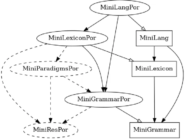
3.2 The Portuguese resource grammar. . . 61
3.2.1 A Portuguese miniresource grammar . . . 62
3.2.3 Extra modules . . . 72
3.2.3.1 Morphological modules . . . 72
3.2.3.2 Grammar extensions . . . 73
3.3 Evaluation . . . 75 3.3.1 UD examples corpus . . . 75 3.3.1.0.1 Copular verbs and adjectives . . . 76 3.3.1.0.2 Copula type in complement of copula . . . 77 3.3.1.0.3 Incorrect trees . . . 78 3.3.1.0.4 Romance clause inversion. . . 79 3.3.1.0.5 Romance clitic pronouns . . . 81 3.3.1.0.6 The no quantifier . . . 82 3.3.2 Matrix MRS test suite . . . 82
3.3.2.1 Discussion . . . 84
3.3.2.1.1 Mismatched tenses . . . 84 3.3.2.1.2 Whose as interrogative . . . 86 3.3.2.1.3 Compound nouns . . . 87 3.3.2.1.4 Adverb placement . . . 87 3.3.2.1.5 Incorrect tense choices . . . 88 3.3.2.1.6 Tag questions . . . 88 3.3.2.1.7 Date and time units . . . 88 3.3.2.1.8 Incomplete sentences. . . 89 3.3.2.1.9 Iberic negative imperatives . . . 89
4 APPLICATIONS . . . 91
4.1 Health-domain application grammar . . . 91
4.2 Attempto Controlled English and GF . . . 91 4.2.1 ACE . . . 92 4.2.2 ACE-in-GF . . . 93 4.2.3 Implementation and example usage . . . 94
4.3 GF to UD . . . 95 4.3.1 Trees . . . 95 4.3.1.0.1 Abstract syntax trees . . . 95 4.3.1.0.2 Parse trees . . . 96 4.3.1.0.3 Dependency trees . . . 96 4.3.1.0.4 Abstract dependency trees . . . 96 4.3.2 The algorithm. . . 96 4.3.2.0.1 Example . . . 98 4.3.2.0.2 Corpus . . . 98 4.3.3 Discussion. . . 100
5 CONCLUSION . . . 103
5.1 Future Work. . . 103 5.1.1 Known issues with the Portuguese RG . . . 103 5.1.1.0.1 Preposition + personal pronoun contractions . . . 103 5.1.1.0.2 Enclitic and mesoclitic pronoun contractions . . . 104 5.1.1.0.3 Preposition + demonstrative pronouns contractions . . . 104 5.1.1.0.4 Reflexive two-place adjectives . . . 104 5.1.2 Possible applications . . . 105 5.1.2.0.1 WordNet gloss corpus . . . 105 5.1.2.0.2 Data as text . . . 106
23
1 Introduction
This thesis presents a computational grammar of Portuguese developed under the Grammatical Framework (GF) formalism. GF is a programming language designed for grammar writing, whose aim is to diminish the cost of creating grammars: it features a robust type-system to catch errors during compile-time (versus having these errors showing up at run-time), an elegant functional programming approach to describing grammars in a generative way [30], a standard library to share and encapsulate common aspects of all natural language grammars [32], and a common, shared ecosystem including the GF compiler, two runtime systems, and a testing tool able to generate minimal and representative test cases for grammatical constructions of choice [23].
Natural language processing tools such as grammars are often faced with a coverage versus correctness tradeoff: tools like Google Translate will produce output for any given input, but their results are often bad (although improving by the day); tools like GF grammars, on the other hand, will not be able to produce output for any input, but when they do they are often correct, or at least easily fixed in most cases (we give several examples of errors that were corrected in section 3.3). Because of GF’s lack of coverage, its main goals are that of domain-specific natural language processing – where the lexicon and linguistic phenomena are more restricted – and that of natural language generation (NLG). Its ideal application in this respect is that of generating grammatically-correct
natural language from data such as ontologies or database entries.
Our GF grammar has the same characteristics of GF as a whole: it is unsuitable for general purpose natural language processing, and thus aims to
1. generate grammatically-correct Portuguese;
2. provide an application-programmer interface capable of supporting domain-specific grammars and applications.
1.1
Motivation
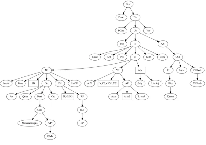
A grammar is a set of rules that govern a language. It tells us how to combine and compose sentences from its constituents. A computational grammar is an encoding of such rules in a way that allows a computer to analyse sentences to its constituents (an analysis which is often represented as a tree like the one in figure 1), or to generate sentences according to these rules (gloss 1 shows a randomly generated sentence from our Portuguese grammar). The act of analysing a sentence string to produce analysis
24 Chapter 1. Introduction
Figure 1 – Constituent analysis of a sentence
trees is called parsing, while transforming an analysis tree into a sentence string is called linearization (or generation). Note that parsing may successfully analyse the sentence string in more than one way or not at all, while the linearization of a well-formed tree will produce at least one sentence tree.
(1) deixe a maior parte de distância ser quebrada, poucos taças de ninguém, distâncias, distâncias a garrafa de muitos copos de ninguém e copos de todo a maior parte de algo falado diretos que não teria sido doente se tais que teria tido fome, que não teriam sido assustados então que serão prontos fáceis a si tais que teria havido francês e se que não tinham estado errados ou que não teriam estado certos, tais que tudo não se chamaria nada, que não serão prontos então que não teriam sido, ou tais que alguém não se teria chamado todos ou tais que ninguém não terá sido ou ou que terão sido prontos, que tinham estado certos ou que estão certos, tais que que todos não terão sido casados com nada porque todos teriam tido sede se tinha tornado mais velho que este esquerda de ninguém e tanto que têm sede eles mesmos e tais que não estava certo quanto tais que teria feito tanto casado
Grammars are useful because the text analyses they produce – be them syntactic or semantic – are a possible way of understanding texts automatically. Of course, grammars are not the only way of producing such analyses (statistical methods of doing so are
1.2. Scope and Contributions 25
actually more popular), nor are they the only way of achieving this ultimate goal of artificial intelligence. Grammars are useful for their introspectability (it is relatively simple to see where mistakes stem from and how to fix them, compared to statistical methods) and for their portability (they encode a lot of information in relatively little space). Grammars do have their problems in incompleteness (they can not parse any given text), cost (writing a grammar is a lot of work) and performance (parsing text can be an expensive operation time- and space-wise). However, as Ranta puts it [33, section 1.3], even though grammars (as abstractions of natural language) leak, all we need to justify them is that they are useful. And their usefulness comes from a very common-sense principle (the title of [39]): don’t guess if you know. This means that there is no need for us to try to determine statistically (i. e., guess) the behaviour of regular, well-known patterns of language (like subject-verb agreement, lemmatization, etc). Let us employ these methods to phenomena which are highly irregular (or which are simply out of our grammar’s scope) instead.
1.2
Scope and Contributions
In this work we present a GF Portuguese grammar in the GF formalism whose linearizations are tested against two GF treebanks. The intended minimal coverage of this grammar is that of all GF Resource Grammar Library constructors (see section 3.1 for details), only including its extensions where they might be needed to generate our test treebanks of choice correctly. A list of the linguistics constructors covered by the RGL can be found at its synopsis1.
Our foremost contribution is the freely-available GF Portuguese grammar (a preview of which appeared in [7]). While unsuitable for general domain parsing, this grammar was able to generate grammatical sentences from the syntactic trees in our test treebanks in more than 90% of the cases (see section 3.3 for details).
In the process of developing it, we have made contributions to the Romance grammar it is based on, which in turn meant contributions for languages such as Spanish and Catalan. We have also made non-academic contributions to the GF community, providing documentation patches and maintenance work (we set up continuous integration testing for the GF repositories and provided documentation fixes, for example).
A complete Portuguese grammar involves not only syntactic coverage but also lexical coverage. To be able to provide a GF dictionary we needed a Portuguese lexicon. Our work in developing MorphoBr [8], a full-form lexicon of Portuguese open class words was inspired by this need.
Because of our work [6,12] involving the Portuguese WordNet, we were naturally inclined to contribute to the gf-wordnet project. We have produced a Portuguese
26 Chapter 1. Introduction
stantiation of this project, based on our GF Portuguese grammar and on the Portuguese WordNet [11]. Although the project (and its Portuguese version) is still ongoing, we were also able to contribute corrections to the Portuguese WordNet.
Finally, we have also made three existing GF applications support the Portuguese language by virtue of our Portuguese grammar. Although most of them are more prototypes than industrial-grade applications, they should give an idea of what GF is capable of. One of these applications is the GF to Universal Dependencies conversion developed by Kolachina & Ranta [20]. This conversion project has created a GF treebank which is used to test both the project itself and the GF grammar library. On top of adding support for Portuguese in this project, we have also revised its treebank, contributing tree corrections and removing duplicate trees.
1.3
Structure
In chapter 2 we aim to acquaint the reader with GF. We first present the ideas behind GF; then we provide an example-based tutorial to familiarize the reader with GF syntax and semantics. We then describe what GF functors are, and how they can be used to generalize grammatical notions, promoting sharing between different concrete implementations. We conclude with a more in-depth view of GF, where we follow Angelov [1] in defining GF mathematically, including how its parsing and linearization work formally. Understanding this last part is not required to understand the remainder of this thesis.
Chapter 3 is the backbone of this work. It presents the GF Resource Grammar Library (RGL), discussing the motivation behind its existence, its uses, and its structure. We then describe our Portuguese implementation of a resource grammar, which is based on the RGL Romance functor. We fully describe a miniature version of a resource grammar for Portuguese, and then discuss the main points of the full implementation, including mor-phology and extension modules. Finally, we evaluate our work under syntactically-correct language generation respect by linearizing two treebanks from well-known computational linguistics projects, analysing errors and discussing potential solutions.
Chapter 4presents three pre-existing GF applications which have been extended to use our Portuguese grammar implementation. The first application is a demonstration of a health-domain translation chat app developed by a company run by the GF core development team. The second application is a mapping from the Attempto Controlled English controlled natural language to GF, which allows one to use GF and the RGL to both parse and linearize ACE-like text in languages other than English itself. The last application is a converter of GF abstract syntax trees to Universal Dependencies (UD) trees [20], which allows GF to be used as rule-based dependency parser, or as a bootstrapper of UD treebanks, among other uses. Our focus is in showing how simple it
1.4. Typesetting Conventions 27
is to add a new language to a GF multilingual app, given a resource grammar for the language is available.
Finally, in chapter5 we summarize our work and discuss future projects.
1.4
Typesetting Conventions
Throughout this thesis we discuss linguistic examples. Single examples are usually typeset inline in italic font, as are linguistic terms. More elaborate examples are typeset as two or three pieces of text like in gloss 2. If there are just two text fragments, the first is an English version, and the second a Portuguese one – whether it is produced from our grammar or is simply an example should be clear from the context. When there are three fragments, the first is the English version, and the following two fragments are Portuguese. It should be clear from the context whether the first Portuguese fragment is the final grammar output – in which case the second fragment is either the ideal output or another possible version – or whether the first Portuguese fragment was the original grammar output before a correction was made, which then produced the second Portuguese fragment.
(2) a. I always thought that there was something fundamentally wrong with the universe
b. eu sempre pensei que havia algo de fundamentalmente errado com o universo
When an example is ungrammatical, we prefix it with an asterisk (*); when the example is grammatical but is the ideal one (where the sense of ‘ideal’ is given by the surrounding context), we prefix it by an exclamation mark (!). Finally, when an example is semantically incorrect but otherwise grammatical, we prefix it by a hash sign (#).
We also typeset inline GF elements differently – including judgement names, modules, constructors, categories, and functions. GF code is shown as in listing 1.1.
−− this is a comment
fun
Hello x = {s = "Hello" ++ x. s} ;
29
2 Grammatical Framework
We begin this chapter with an overview of GF. We proceed to a short tutorial on GF, whose purpose is to make the reader familiar with GF syntax and semantics. We conclude the chapter by giving a mathematical definition of an important subset of GF, and showing formally how parsing and linearization are done in it.
Grammatical Framework (GF) is a domain-specific programming language for grammar writing. It is a functional programming language, with syntax inspired by the Haskell programming language [25]; it draws from intuitionistic type theory [26] for its type system.
A GF program is called a grammar, and it defines parsing, generation and translation from the same declarative source.
GF’s forte lies at multilingual processing. It applies to natural languages the distinction made for programming languages: that of an abstract and a concrete syntax. Separating them allows GF to specify a single abstract grammar for several concrete languages. Translation between two natural languages, for instance, becomes parsing of concrete syntax to its abstract representation, and then further linearization to the target language.
Foods> parse -lang=Eng "this fish is fresh" Pred (This Fish) Fresh
Foods> parse -lang=Por "este peixe é fresco" Pred (This Fish) Fresh
Foods> linearize -all Pred (This Fish) Fresh this fish is fresh
este peixe é fresco
The idea is that both sentences above carry the same (abstract) information, which is represented in each language by the respective string. A GF grammar demands a description of its abstract syntax and how this syntax translates into the concrete syntaxes, i.e., the strings. The abstract syntax encompasses both trees (such as [Pred (This Fish) Fresh]) and their construction rules (see listing 2.1 for an example of an abstract GF grammar). The concrete syntaxes, on the other hand, must specify rules for the translation of trees into strings of the desired language. Although natural languages are the main focus, GF can and has been used to generate any kinds of strings, e.g. LATEX code. Listing2.2
30 Chapter 2. Grammatical Framework
version of the Foods grammar appearing in GF documentation and literature, for example in [33, chapter 3].
abstract Foods = { cat
Comment ; Item ; Kind ; Quality ;
fun
Pred : Item → Quality → Comment ; This : Kind → Item ;
Fish : Kind ; Fresh : Quality ; } ;
Listing 2.1 – Abstract grammar Foods.
concrete FoodsEng of Foods = { lincat
Comment, Quality = {s : Str} ; Kind = {s : Number ⇒Str} ; Item = {s : Str ; n : Number} ;
lin
Pred item quality =
{s = item.s ++ copula ! item.n ++ quality . s} ; This = det Sg "this " ;
Fish = noun "fish" " fish " ; Fresh = adj " fresh " ; param
Number = Sg | Pl ; oper
det : Number →Str →
{s : Number ⇒Str} → {s : Str ; n : Number} = λn,det,noun → {s = det ++ noun.s ! n ; n = n} ; noun : Str → Str → {s : Number ⇒Str} =
λman,men →{s = table {Sg ⇒man ; Pl ⇒ men}} ; regNoun : Str → {s : Number ⇒Str} =
λcar → noun car (car + "s") ; adj : Str → {s : Str} =
λcold → {s = cold} ; copula : Number ⇒Str =
table {Sg ⇒ " is " ; Pl ⇒ "are"} ;
} ;
Listing 2.2 – Concrete English grammar for Foods.
2.1
A GF tutorial
In this short tutorial we give an overview of GF as a programming language. We refrained from using an example in the natural language domain, because any such
2.1. A GF tutorial 31
example would need to be much simplified for our current purpose of presenting GF syntax and semantics. Therefore we opt for a complete example which has the added benefit of being familiar to most programmers. The linguistics-inclined reader will have to wait until chapter 3 for linguistically-motivated GF code.
By the end of this section we expect the reader to be able to read and understand GF with reasonable fluence, even if writing it is another matter. Despite this stated goal, we still offer information which might be useful to the reader who intends to learn GF, e. g., how to use the GF shell. To this kind of reader we recommend following the examples in your computer, with GF installed.
The definitive resource to learn GF is the GF book [33]; the freely-available online reference1, from where we take many of the definitions in this section, is also useful to look
up syntactic or semantic details; finally, Inari Listenmaa’s blog post2 is a great resource to
avoid common GF pitfalls.
2.1.1
A simple GF grammar
In this section we present a grammar for linked lists, capable of translating between two different syntaxes for them. The Lisp syntax uses () for the empty list and represents a non-empty list as a series of elements separated by spaces, delimited by parentheses on both ends, like so: (0 1 1 2 3 5). The Haskell syntax uses [] for the empty list, while non-empty lists are elements separated by commas (with optional spaces), delimited by square brackets on both ends, as in [0,1,1,2,3,5] .
Linked lists are a data structure which is defined recursively. A list is either:
(1) the empty list (also called Nil); or
(2) a list with an element added at the front.
Because adding an element to the front of a list is how you construct all lists except for the empty one, this process is called Cons. Given this definition, Cons X (Cons X (Cons X Nil)) is an abstract tree representing the three-element list which in Lisp syntax is
(x x x).
A GF grammar is composed of an abstract syntax and any number of concrete syntaxes. While the abstract syntax declares categories and how they can be combined as in a logical framework, the concrete syntaxes define the linearization of the created abstract syntax trees to strings.
1 http://www.grammaticalframework.org/doc/gf-refman.html 2 https://inariksit.github.io/gf/2018/08/28/gf-gotchas.html
32 Chapter 2. Grammatical Framework
Each GF module is composed by a header3 and a body, which is simply a set
of judgements. The GF compiler demands that the programmer specify what form of judgement she is making by using a judgement keyword, so, e.g., we precede category declarations with cat. We may specify a judgement keyword for each judgement, or (more conveniently) we may omit subsequent judgement keywords of the same form. Each
judgement is separated by a semicolon (;).
Listing 2.3 shows an abstract syntax for linked lists in GF syntax. Note how it follows the recursive definition of lists. We use the cat judgement to declare categories; it has the form cat C.4 In this example, we define the List category that we are interested in, and a dummy element category Elem. We also add the S (for sentence) category, which is special in GF in that it is the default start category for a grammar. The start category is the category we start parsing from. The fun judgment declares how we can construct a member of a category from members of its argument categories; it has the formfun f : T, where T is a type built from basic types (i. e., declared categories and built-in categories like Str) using the type constructor→. We declare two zero-argument constructors (which are constants) and the Cons constructor which is the same as in the recursive definition of lists. To be able to parse lists from the start category S, we add the LSconstructor, which lifts lists to the sentence category.
abstract List = { cat Elem ; List ; S ; fun X : Elem ; Nil : List ;
Cons : Elem → List → List ; LS : List → S ;
} ;
Listing 2.3 – Abstract syntax for linked lists in GF.
We can already import the file List.gf5 in the GF shell, and play with the
generate_trees and generate_random commands. Note that all GF shell commands have shorter aliases. To know more about GF shell commands, call help for a summary of all available commands, or help [command], for help on the command [command].
3 Module headers specify what kind of module it is, imports, and other things; See the GF reference
at [33] orhttp://www.grammaticalframework.org/doc/gf-refman.htmlfor more about headers.
4 This form is actually a simplification; for the dependently-typed subset of GF we use more elaborate
category declarations.
2.1. A GF tutorial 33
> i List . gf
List > gt −number=3
Cons X (Cons X (Cons X (Cons X Nil))) Cons X (Cons X (Cons X Nil))
Cons X (Cons X Nil)
Listing 2.4 – GF shell session with abstract module only.
In order to implement a concrete syntax for this abstract syntax, we must ask ourselves how we want to linearize each constructor defined in the abstract syntax. If we take Lisp lists as an example, we want to have
Nil <=> () Cons X (Cons X (Cons X Nil)) <=> (x x x)
In order to achieve this behaviour, we first have to define the linearization types of the categories declared in the abstract module, using the lincat judgement keyword, as in listing 2.5.
concrete ListLisp of List = { lincat
Elem, S = {s : Str} ; List = {bp,b : Str} ;
Listing 2.5 – Lisp list linearization types.
lincat judgements are composed of category names, an equal sign (=), and a valid linearization type. A linearization type can be either a basic type, a parameter type (user-or library-defined), a table and/(user-or rec(user-ords of those, but not a function type (we will explain these shortly). We decide on the ElemandStypes being a record type with one field of Str type, and on the List type being a record with two string fields, bpto store the beginning parenthesis, and b to store the body of the list (see listing2.5).6 If more than one category
share a linearization type, we can define them in a single judgement by separating the category identifiers by commas.7 We may also omit the linearization type of a category,
which gives it the default {s : Str} linearization type.
Listing 2.6contains the actual linearizations. The dummy X element is linearized to "x", Nil is linearized to a record containing the strings for ( ), and Cons updates
6 We could make ElemandS
be simple Str types, however it is a GF convention to use record types for their extensibility – it is much easier to add a field to an existing record than to change something into a record and then add a field to it.
7 Something analogous works in abstract modules for the declaration of several constructors of the same
34 Chapter 2. Grammatical Framework
(∗∗) its second argument (the list argument) with a new body field consisting of the concatenation (++) of the string field of the element argument (x) and of the body field of list argument (xs). The extension record operator ∗∗ is used to both extend and update records; it essentially performs the union of the records’ fields. When the two records’ field labels are not disjoint, the second record’s fields get precedence, essentially updating the values of the first record’s fields. Our use of ∗∗ could have been written equivalently asCons x xs = {bp = xs.bp ; b = x.s ++ xs .b}. We finally define LS to simply be the concatenation of the beginning parenthesis with the body of the input list.
lin X = {s = "x"} ; Nil = {bp = "("; b = ")" } ; Cons x xs = xs ∗∗ { b = x.s ++ xs .b } ; LS xs = {s = xs.bp ++ xs .b} ;
Listing 2.6 – Lisp list linearization rules.
> i ListLisp . gf
List > parse −lang=Lisp "( x x x x )" LS (Cons X (Cons X (Cons X (Cons X Nil))))
Listing 2.7 – GF shell session with single concrete module.
Now let’s define another concrete syntax, this time for Haskell lists. We want to have:
Nil <=> [] Cons X (Cons X (Cons X Nil)) <=> [x,x,x]
There is an issue here with the commas. We only want to insert a comma when there is an existing element in the input list (i. e., the input list is not the empty list). If we try to define Cons as something similar to the Lisp definition in listing 2.6, but with a comma in-between the concatenation of the elements (as in x. s ++ " , " ++ xs .b), we will get the wrong linearization when the input list is empty. To solve this problem, we give lists a more complex linearization type, as can be seen in listing 2.8.8 For this, we
introduce the param judgement, which is used to declare a new parameter type, together with its constructors. A parameter type is either introduced by a param judgement or is a
8 We could have solved this problem by creating a separate category of empty lists, but this has two
downsides: it makes the Lisp concrete more complicated than it has to be, and it does not follow precisely the recursive definition of linked lists. An additional downside is that it prevents the introduction of useful GF concepts to the reader.
2.1. A GF tutorial 35
record type whose fields are all parameters types. Parameter types must be finite (we may not have a parameter constructor take an infinite type such as a string as an argument) and thus non-recursive.
param
Boolean = T | F ;
lincat
Elem, S = {s: Str} ;
List = {s : Str ; null : Boolean} ;
Listing 2.8 – Haskell List linearization types.
We define a boolean parameter whose values might beT andF (for true and false), and make it the type of a field in the linearization type of lists. This will allow us to give different linearizations to different values of the null field. The reader may have noticed that the bp field of Lisp lists was always the same; to remove this redundancy in the Haskell concrete we remove the bp field, and rename the b field to s. We use the LS rule to add the beginning square brackets of the lists. The linearization rules of Haskell linked lists can be seen in listing 2.9.
lin X = {s = "x"} ; Nil = { s = "]" ; null = T } ;
Cons x xs = case xs.null of {
T ⇒ {s = x.s ++ xs . s ; null = F} ; _ ⇒ xs ∗∗ {s = x.s ++ " , " ++ xs . s} } ;
LS xs = {s = "[" ++ xs . s} ;
Listing 2.9 – Haskell List linearization rules.
Cons’s linearization rule introduces GF case expressions, which allows us to pattern-match on parameter values. GF case expressions are simply syntactic sugar for table selections. GF tables are finite functions of type P ⇒ T , where P is a pa-rameter type and T is any type. Tables can be written with the table keyword like so:
table { V1 ⇒ t1 ; ... ; Vn ⇒ tn }, where the V’s are parameters and the t’s are expres-sions of the output type of the table. Tables are finite functions because parameter types are themselves finite, so it is possible to enumerate all input-ouput pairs. You can apply a table to an expression that evaluates to an instance of its input parameter type using the table selection operator !.
36 Chapter 2. Grammatical Framework
Becausecaseis just syntactic sugar for tables, the linearization of Cons in listing2.9 is equivalent to the one in listing2.10 (note the use of the record selection operator). The underscore (_) is called a wildcard pattern and matches any value.
Cons x xs = table {
True ⇒xs ∗∗ {s = x.s ++ xs . s ; null = F} ;
_ ⇒ xs ∗∗ {s = x.s ++ " , " ++ xs . s} } ! xs . null
Listing 2.10 – Cons linearization rule using GF tables.
In order to linearize Cons, then, we check if its list argument is the empty list by checking its null field; if it is, we update its s field with the concatenation of the element string field and its current s field (which is just the closing square bracket). Its null field is also updated, to the value ofF, indicating that the list is not empty anymore. If the list argument is not an empty list, we simply update its body field to be the concatenation of the string field of the element argument, a comma, and its previous body field. The other linearization rules are what one would expect.
Now that we have two concrete syntaxes, we can translate between them by parsing one concrete to the abstract syntax and then linearizing the abstract tree to the target concrete syntax:
> i ListLisp . gf ListHask . gf
List > p −tr −lang=Lisp "( x x x )" | l −lang=Hask Cons X (Cons X (Cons X Nil))
[ x , x , x ]
Listing 2.11 – Translation between List concrete syntaxes.
The -tr option of a GF shell command traces its output (i.e., prints it), while the pipe command (|) uses the output of the previous command as the input to the next one.
2.1.2
Refactoring
If we analyse the two concrete grammars we developed in section 2.1.1, we can see that they share many definitions, like that of the lincat of Elem or that of the LS constructor. As a functional programming language, GF has the means to avoid most code boilerplate and repetition. Two of the most prominent ways of doing so is by using functors and the oper judgement. In this section we refactor our implementation of the List grammar using both of these. Note that the gains of using these GF constructs in such a small grammar are negligible, but that they are very useful in larger grammars.
2.1. A GF tutorial 37
An oper is akin to a function definition in most programming languages. It is of the form oper h : T = t, where T is a type and t is a term of type T. The type can be omitted if the compiler is able to infer it, and type and definition can also be given by two separate oper judgements. Note that in many cases the term definition t of an oper will be an anonymous function (or lambda abstraction) of the form λx → t, which is a one-argument function whose application is computed by substituting its argument for x
in t. Listing 2.12shows the declaration and definition of an oper consWith that can be used to avoid the repetition in the two branches of the case expression in the previous definition of the Cons constructor, as is done in listing 2.14. It is also possible to define an oper using a shorthand like the one used by lin judgements.
oper
consWith : Str → Elem → List → List
= λsep,x,xs → xs ∗∗ {s = x.s ++ sep ++ xs . s ; null = False} ;
−−−− could also be defined as two separate judgements: −− consWith : Str → Elem → List → List ;
−− consWith sep x xs = xs ∗∗{s = x.s ++ sep ++ xs . s ; null = False} ;
Listing 2.12 – Cons using a consWith oper
In larger GF grammmars it is customary to define parameters and functions in a resource module, which can then be imported by several concrete modules for use.
The other element used in our refactoring of the List grammar are functors. GF functor modules are inspired by the parametrized modules found in functional programming languages like ML.9 A GF functor module is any module that opens (imports) an interface
module. An interface module is a module that only declares oper judgements, possibly defining them.
The header syntax for a functor module is like below:
incomplete concrete ListI of List = open ListSyntax in
The incomplete keyword highlights the fact that a functor without its instantiation is not a valid (concrete) grammar. The ListSyntax module is the interface module that is opened by the functor.
What allows wider use of functors is the possibility of using abstract syntax modules as interface modules, and concrete syntax modules as their instances, performing the following mapping:
cat C ↔ oper C : Type
9 If you know the functional programming language Haskell, be warned: its functors are a different
38 Chapter 2. Grammatical Framework
fun f : A ↔ oper f : A
lincat C = T ↔ oper C : Type = T
lin f = t ↔ oper f : A = t
To refactor our list grammar into a functor, we try to generalize our two original implementations, trying to abstract what they do not have in common to the interface module. In the case of lists, we know that Haskell and Lisp syntax differ only in what kind of separator they use and what kind of boundary characters they use, so we end up with the ListI functor module in listing2.14 and the ListSyntax interface module in listing2.13. In order to build ListI, we took the most general implementation out of the two (that of Haskell), and changed a few strings to parametrized opers, which are declared in ListSyntax. To complete our implementation, we only need to instantiate both modules for each concrete we want, which we do in figure2. Because the type signatures of the opers are already given in the interface module, we do not need to give them in its instantiations.
We can think of the List functor module as a function at the module-level, with a type signature like:
ListI : instance of ListSyntax → concrete of List
Functor instantiation then would resemble function application.
interface ListSyntax = { oper elemSep : Str ; leftBound : Str ; rightBound : Str ; } ;
Listing 2.13 – List syntax interface module.
2.2
GF, mathematically
GF grammars can be compiled to a binary format called portable grammar format (PGF) [2]. This format is ideal for a formal description of GF since it abstracts away syntactic details of GF as a programming language. In this section we present the mathe-matical definition of this format, discuss on a high-level how GF code is translated into it, and show how parsing and linearization is done by a PGF interpreter. The main source for this section is Krasimir Angelov’s PhD thesis [1], which we follow closely in text and notation; we have contributed nothing to his work.
2.2. GF, mathematically 39
instance ListSyntaxHask of ListSyntax = { oper
elemSep = "," ; leftBound = "[" ; rightBound = "]" ; } ;
Listing 2.15 – Haskell list syntax instantiation.
concrete ListFHask of List = ListI
with ( ListSyntax=ListSyntaxHask) ∗∗{ } ;
Listing 2.16 – Haskell list functor instantiation.
instance ListSyntaxLisp of ListSyntax = { oper
elemSep = "" ; −− no element separator but for spacing
leftBound = "(" ; rightBound = ")" ; } ;
Listing 2.17 – Lisp list syntax instantiation.
concrete ListFLisp of List = ListI
with ( ListSyntax=ListSyntaxLisp) ∗∗ { } ;
Listing 2.18 – Lisp list functor instantiation.
40 Chapter 2. Grammatical Framework
incomplete concrete ListI of List = open ListSyntax, Prelude in {
lincat
Elem, S = {s : Str} ; List = {
s : Str ;
−− Bool is actually a pre−defined parameter type, so we don’t −− need to redefine it null : Bool } ; lin X = {s = "x"} ; Nil = { s = rightBound ; null = True } ;
Cons x xs = case xs.null of {
True ⇒consWith "" x xs ;
_ ⇒ consWith elemSep x xs } ;
−− we can use lambda abstractions for lin definitions too!
LS = λxs → {s = leftBound ++ xs . s} ; oper
consWith : Str → Elem → List → List
= λsep,x,xs → xs ∗∗ {s = x.s ++ sep ++ xs . s ; null = False} ;
−−−− could also be defined as two separate judgements: −− consWith : Str → Elem → List → List ;
−− consWith sep x xs = xs ∗∗{s = x.s ++ sep ++ xs . s ; null = False} ;
} ;
Listing 2.14 – List functor module.
We only present a subset of GF in that we don’t discuss dependently-typed GF code.
2.2.1
Definitions
Definition 1. A PGF grammar G is a pair of an abstract grammar A and a finite set of concrete syntaxes C1, . . . , Cn:
G = hA, {C1, . . . , Cn}i
Definition 2. An abstract syntax is a triple of a set of abstract categories,10 a set of
2.2. GF, mathematically 41
abstract constructors with their type signatures, and a start category:
A = hNA, FA, Si
• NA is a finite set of abstract categories.
• FA is a finite set of abstract constructors. Every element in the set is of the form
f : τ where f is a constructor symbol and τ is its type. The type is either a category C ∈ NA or a constructor type τ1 → τ2 where τ1 and τ2 are also types.
• S ∈ NA is the start category.
Definition 3. A concrete syntax C is a parallel multiple context-free grammar (PMCFG) complemented by a mapping from its categories and constructors to the abstract syntax:
C = hG, ψN, ψF, di
• G is a PMCFG: an extension of a context-free grammar (CFG) where a syntactic category is defined not as a set of symbols but as a set of tuples of strings. We apply constructors over tuples of input categories to obtain a tuple in the result category. A formal definition of PMCFG is given in definition 4, but a PMCFG is mainly composed of a set of production rules which define how to construct a given category by applying some constructor. An example using a constructor f and categories A, B, and C is the production rule:
A → f [B, C]
• ψN is a mapping from the concrete categories in G to the set of abstract categories NA.
• ψF is a mapping from the concrete constructors in G to the set of abstract constructors FA. A concrete constructor fC has the same arity of its corresponding abstract constructor:
a(fC) = a(ψF(fC))
where a is a mathematical function which takes a GF constructor and returns its arity.
The notation for the definitions of concrete funtions is tailored to simplify the deduction rules we will write later; an example is:
42 Chapter 2. Grammatical Framework
where f is the constructor name. The notation hd; ri stands for the constituent number r of argument d, so f creates a tuple of two strings where the first one (h0; 0ib) is built from the first constituent of the first argument and by adding the terminal b at the end. The second one (h1; 0ih0; 1i) concatenates the first constituent of the second argument with the second constituent of the first argument of the first argument.
• d assigns a positive integer d(A), called dimension, to every abstract category A ∈ NA.
A given category may have different dimensions in the different concrete syntaxes.
Definition 4. A parallel multiple context-free grammar (PMCFG) [36,37] is a 5-tuple:
G = hNC, T, FC, P, Li
• FC is a finite set of concrete categories. For every A ∈ NC, the equation d(A) =
d(ψN(A)) defines the dimension for every concrete category as equal to the dimension in the current concrete syntax of the corresponding abstract category.
• T is a finite set of terminal symbols.
• FC is a finite set of concrete constructors. For every f ∈ FC, the dimensions r(f )
(the number of constituents in the output of f ) and di(f ) (the dimension of the i-th argument category) (with 1 ≤ i ≤ a(f )) are given. For every positive integer d, (T∗)d denotes the set of all d-tuples of strings over T . So if T = {a, b}, then (T∗)3 = {(a, a, a), (a, a, b), (a, b, a), (b, a, a), (b, b, a), (b, a, b), (a, b, b), (b, b, b)}. Each
constructor f ∈ FC is a total mapping from (T∗)d1(f )× (T∗)d2(f )× · · · × (T∗)da(f )(f )
to (T∗)r(f ), and is defined as
f := (α1, α2, . . . , αr(f ))
Here αi is a sequence of terminals and hk; li pairs, where 0 ≤ k ≤ a(f ) is called argument index and 0 ≤ l ≤ dk(f ) is called constituent index. We also use the notation rhs(f, l) to refer to constituent αl of the constructor f .
• P is a finite set of productions of the form:
A → f [A1, A2, . . . , Aa(f )]
where A ∈ NC is called result category, A1, A2, . . . , Aa(f ) ∈ NC are called argument categories and f ∈ FC is a constructor symbol. For the production to be well formed, the conditions di(f ) = d(Ai) (with 1 ≤ i ≤ a(f )) and r(f ) = d(A) must hold.
2.2. GF, mathematically 43
• A default linearization function L of a category C is a function which produces an object of the linearization type of C when applied to a string. L ⊂ NC× FC is a set
which defines the default linearization functions for those concrete categories that have default linearizations. If the pair (A, f ) is in L then f is a default linearization function for A. We will also use the abbreviation:
lindef(A) = {f | (A, f ) ∈ L}
to denote the set of all default linearization functions for A. For every f ∈ lindef(A) it must hold that r(f ) = d(A), a(f ) = 1, and d1(f ) = 1.
The abstract syntax defines a grammar of typed lambda terms; similarly, the concrete syntaxes allow us to construct concrete syntax trees:
Definition 5. (f t1. . . ta(f )) is a concrete tree of category A if ti is a concrete tree of category Bi and there is a production:
A → f [B1. . . Ba(f )]
The abstract notation for to say that t is a tree of category A is t : A. When a(f ) = 0, then the tree does not have children and the node is called a leaf.
A concrete syntax tree can be bottom-up linearized to a tuple of strings in the following way: leaves (trees with no arguments) are already tuple of strings; to linearize a tree with one or more arguments, one linearizes the arguments first, and them combines the linearization into a tuple of strings.
To define a linearization procedure, we employ a helper constructor K which produces a string from a sequence of tuples of strings (the linearized arguments) and a sequence αi of terminals and hk; li pairs. The output string is produced by the substitution of each hk; li with the string for constituent l from argument k:
K −→σ (β1hk1; l1iβ2hk2; l2i . . . βn) = β1σk1l1β2σk2l2. . . βn
where βi ∈ T∗ and −→σ is the sequence of linearized arguments. With K, we can define L, the actual linearization constructor:
L (f t1t2. . . ta(f )) = (x1, x2, . . . xr(f )) (2.1) where
xi = K (L(t1), L(t2) . . . L(ta(f ))) αi and
44 Chapter 2. Grammatical Framework
2.2.2
From GF to PGF
In this section we discuss on a high level how GF code is transformed into PGF. As shown in section 2.2.1, the PGF format is very simple – its production rules simply generate tuples of strings from other tuples of strings. So it is natural to ask how the GF compiler can encode the relatively rich language of GF in this simpler system.
The first thing to notice here is that although GF enjoys pattern-matching and function definitions (opers), these are compiled away when GF is transformed into canonical GF [24,30], which is a variant of GF without syntactic sugar and where partial evaluation has been applied. To partially evaluate GF code means to inline all functions definitions, and evaluate all expressions as far as possible, until they depend on runtime variables (as constructors do). This is possible because GF functions may not be recursive nor co-recursive. We can also compile away pattern-matching because GF parameter types (on which we pattern match) are finite, and can thus be enumerated. Canonical GF then only has category and constructor declarations and definitions, containing only argument variables, strings, records, tables, and parameters, plus the concatenation, record projection and table selection operators. Thus we only have to worry about converting these to PGF. Records and tables can be straightforwardly flattened to tuples of strings. However it is not so clear how can we encode record fields whose values are parameters, nor how the appropriate elements of tables are selected using parameters.
Let us take the Haskell concrete of the List grammar from section2.1.1as an example grammar being converted to PGF. The Elem category is straightforwardly represented as a one-element string tuple. For instance, X is just "x"; if we had other Elems, they’d be simple strings too. The way to represent a record where one field is a parameter (like in the case of the List category) is to enumerate all possible values of the parameter (which is always possible since parameters must be finite), and create a new concrete category for each such value. Therefore what was just one category in GF (List) becomes two concrete categories in the PGF representation: Listempty and Listnonempty.11 Both
concrete categories are then represented as one-element tuple of strings; the value of their
null fields is encoded by the concrete category they belong to. For example, Nil is then represented as just h")"i.
Now that we know that categories can get split in the GF to PGF conversion, it is easier to see how the linearization definition of the Cons constructor in the Haskell concrete of the List grammar (see listing2.9) is handled. It contains a case expression whose value depends on the two-valued Bool parameter from the null field of its input argument of List. But there is no List category anymore, so we split the Cons constructor into two concrete constructors: one which takes a Listempty and another that takes a Listnonempty.
There is no caseexpression in any of them (and there could not be, nor is there a need to
2.2. GF, mathematically 45
be). For example, the Consnonempty concrete constructor takes a non-empty List as input,
and produces a non-empty List; we know that non-empty Lists are just a one-string tuple; using the notation from definition 3, we have:
Consnonempty := (h0; 0i“,"h1; 0i)
That is, we produce the first constituent (corresponding to the s field) of the one-element tuple by concatenating the first constituent of the first argument (which is an Elem), a comma, and the first constituent of the second argument (which is a Listnonempty).
We can obtain a human-readable PGF from any GF grammar by using the print_grammar command of the GF shell. Its output is very close in notation from the one presented here.
In summary, although PGF preserves abstract categories and constructors defined in GF, it replaces linearization categories and rules by concrete categories and constructors. In the general case there is more than one concrete category and constructor to each linearization category and rule (and thus to each abstract category and constructor). We use ψN and ψF from definition 3 to preserve the mapping from concrete categories to abstract categories and from concrete constructors to abstract constructor, respectively.
2.2.3
Parsing
In this section we show how GF parsing from a PGF representation works using a running example. We first explain the idea behind the parse algorithm, show how we can represent it as a series of deduction steps, and explain the deductions rules we use. We then present the example grammar, and show a complete parse. More details and proofs of soundness (i. e., it is impossible to parse a string not accepted by the grammar) and completeness (i. e., it is possible to parse every string produced by the grammar) of the parsing algorithm can be found in Krasimir Angelov’s thesis [1].
2.2.3.1 The example grammar
Our running example is still that of Haskell lists from section 2.1.1. Figure3 shows the PGF version of the Haskell list grammar from section 2.1.1.
There are two construction rules for the top-level category S (whose dimension is one), one which takes one argument of category N (for empty lists, formerly Listempty), and
another which takes one argument of category L (for non-empty lists, formerly List).Both rules use the same constructor ls, which concatenates the beginning square bracket with its first argument’s first constituent.12 As discussed in section 2.2.2, the Cons becomes 12 The actual PGF has the ls constructor accept a single category of L*, and adds two coercions from
46 Chapter 2. Grammatical Framework S → ls[N ] S → ls[L] L → ce[E, N ] L → co[E, L] N → nl[] E → e[] ls := (“[”h0, 0i) ce := (h0, 0ih1, 0i) co := (h0, 0i“, ”h1, 0i) nl := (“]”) e := (“x”)
Figure 3 – The PGF grammar for Haskell lists.
S → “[”L
L → “]” | “x”L | “x”“, ”L
Figure 4 – A context-free aproximation for Haskell lists without an intermediary category for empty lists
two concrete constructors: one that takes empty lists (ce), and the other which takes non-empty lists (co); the former simply concatenates the first constituent of the first argument (the element) to the first constituent of the second (the list) argument; the latter includes a comma between these two constituents. The element category has only one nullary constructor e, which is a single tuple; the PGF-only empty list category also has a single nullary constructor nl.
The syntax tree for the string [x, x] is (ls (ce e (co e nl))), while that of the empty list is simply (ls nl).
2.2.3.2 The algorithm
GF’s parsing algorithm is a generalization of a context-free parsing algorithm. Figure4 shows a context-free approximation of the grammar Haskell lists that does not use an intermediate category for the empty list.13
To restrict this grammar so that it only produces syntactically correct Haskell lists, we can create new production rules and categories at every rule application. This
13 It is possible to define the grammar exactly using a CFG by adding a category for empty lists; if we
2.2. GF, mathematically 47 S → “[” L L → “]” | “x” L | “x, ” L 1 S 2 “[” L 3 “[” “x, ”L1 L1 → “x” | “x, ” L2 4 “[” “x, ” “x” L2 L2 → “]” 5 “[” “x, ” “x” “]”
Figure 5 – Parse for the string [x , x] using CFG approximation with on-the-fly special-ization.
on-the-fly specialization of the parser prevents it from accepting strings which are not in our example grammar.
Figure 5 shows how parsing the list string [x, x] would work. We begin the parse from the start category S, which has only one branch, so we parse the beginning square bracket, and soon find the L category, which might be formed in three ways; we continue with the only one matching our input in step 3. Now, given that we have parsed an element-with-a-comma, we want to have only two valid continuations: we can either parse the another element-with-a-comma, or we can parse a normal element; this is enforced by the on-the-fly creation of a new category L1 – a specialization of L that does not have
the ending square bracket branch. We continue with parsing the normal element branch (because it matches our input), which means there is no following element – the list must end now or the parse will fail – so we want to have only one valid continuation where we parse the ending square bracket – this is reflected by the new specialized rule L2. Notice
that if we had a malformed input which had another element at this point, the parse would fail; if we were using our pure CFG approximation, the former case would still be parsed. We successfully parse an ending square bracket because it matches our input, and have now fully consumed the input with a successful parse.
A parser for this grammar would look like parser for a context-free language, except for the creation of new categories and rules on-the-fly.
2.2.3.3 Parsing as deduction
We present the parsing algorithm as a deduction, following Shieber et al. [38] Each rule application derives a set of items:
X1. . . Xn
Y hside conditions on X1. . . Xni
where the premises Xi are items, and the derivation Y is also an item. We take the input string to be a sequence w1. . . wn of tokens.
We first explain the kind of items derived by the parser. After presenting the formal notation, we show concrete examples to help make the notation clearer. If these examples
48 Chapter 2. Grammatical Framework
are not enough, their use in section 2.2.3.4 should be enough to explain their significance. We finally present and explain the parsing deduction rules; their use in section 2.2.3.4 should help clarify their semantics.
The parsing deduction system generates active, passive, and production items.
2.2.3.3.1 Production items
In Shieber et al. deduction systems, the grammars are constant. Because in the case of GF parsing the grammars are extended at runtime (as intuited by section2.2.3.2), the set of productions must be a part of the deduction set, and the productions from the original grammar are considered axioms included in the initial deduction set.
2.2.3.3.2 Active items
Active items represent the parsing state at a given point of the deduction:
[kjA → f [−→B ]; l : α • β], j ≤ k
This notation encodes a constructor f with the following production:
A → f [−→B ]
f := (γ1, . . . , γl−1, αβ, . . . , γr(f ))
such that the tree (f t1. . . ta(f )) will produce the substring wj+1. . . wk as prefix in con-stituent l for any sequence of arguments ti : Bi. The sequence α is the part that produced the substring:
K (L(t1), L(t2) . . . L(ta(f ))) α = wj+1. . . wk and β is the part that is not processed yet.
Take the following example active item from a parsing using the Haskell list grammar at figure3 (page46):
[11L → ce[E, N ]; 0 : • h0, 0i h1, 0i]
It denotes the ongoing parse of a non-empty list (category L), starting at index 1 of the input (the lower 1) and currently at index 1 of the input (it has not successfully parsed anything yet). Note that all indices start from zero. This non-empty list is being built from the ce constructor, which takes an element (category E) and an empty list (category N). It is currently parsing the first (thus 0) and only constituent of the result category; its point is just before two argument-constituent pairs corresponding to the first constituent of the first argument and to the first constituent of the second argument. The components after the constituent index correspond exactly to the ones at the ce rule at figure 3.
2.2. GF, mathematically 49
2.2.3.3.3 Passive items
Passive items are written as:
[kjA; l; N ], j ≤ k and are proof of at least one production:
A → f [−→B ] f := (γ1, γ2, . . . , γr(f ))
and a tree (f t1 . . . ta(f )) : A such that the constituent with index l in the linearization of the tree is equal to wj+1. . . wk. Contrary to the active items in the passive the whole constituent is matched:
K(L(t1), L(t2) . . . L(ta(f ))) γl = wj+1. . . wk
Every time there is a completion of an active item, a passive item is derived along with a new category N which accumulates all productions for A that produce the wj+1. . . wk substring from constituent l. All trees of category N must produce wj+1. . . wk in the constituent l.
Observe the following passive item from a parse using the grammar at figure 3 (page 46):
[21E; 0; C0]
It witnesses the parsing of the first (and only) constituent of a member of category E. It spans one token of the input, starting at index 1. It has also produced a specialized category C0 with the production rule C0 → e[], where e is the zero-argument constructor
from figure 3. Its corresponding tree e : E is such that the constituent with index 0 in the linearization of this tree (“x”) is equal to token of the index 1 of the input.
The deduction rules of the parsing system are shown in figure 6.
2.2.3.3.4 Initial predict
Derive an item spanning the 0–0 range for each production whose result category is mapped to the start category in the abstract syntax.
2.2.3.3.5 Predict
Given an active item with a dot before an argument-constituent pair hd; ri and a matching production rule, derive an active item where the dot is in the beginning of the constituent r of the constructor function.
50 Chapter 2. Grammatical Framework
Initial Predict
A → f [−→B ]
ψN(A) = S, S the start category in A, α = rhs(f, 1) [00A → [−→B ]; 1 : •α] Predict Bd→ g[ − → C ] [kjA → [−→B ]; l : α • hd; riβ] γ = rhs(g, r) [kkBd→ g[ − → C ]; r : •γ] Scan [kjA → f [−→B ]; l : α • sβ] s = wk+1 [k+1j A → f [−→B ]; l : αs • β] Complete [kjA → f [−→B ]; l : α•] N = (A, l, j, k) N → f [−→B ] [kjA; l; N ] Combine [ujA → f [−→B ]; l : α • hd; riβ] [kuBd; r; N ] [jkA → f [−→B {d := N }]; l : αhd; ri • β]
Figure 6 – Parsing deduction rules
2.2.3.3.6 Scan
Given an active item with a dot before a terminal s and that s matches the current element wk of the input string, derive a new active item where the dot is moved to the next position.
2.2.3.3.7 Complete
Derive a passive item from an active item whose dot is at the end. The resulting category N in the passive item is a fresh category. Also derive a new production for N which has the same constructor and arguments as the category in the active item.
2.2.3.3.8 Combine
Derive an active item from matching active and passive items. For the purposes of Combine, an active item matches a passive one if its dot is before the parsing of the r-th


![Figure 5 – Parse for the string [x , x] using CFG approximation with on-the-fly special- special-ization.](https://thumb-eu.123doks.com/thumbv2/123dok_br/17339910.795040/49.892.134.803.128.355/figure-parse-string-using-approximation-special-special-ization.webp)

![Figure 7 – Parse deduction for the string [x , x]](https://thumb-eu.123doks.com/thumbv2/123dok_br/17339910.795040/54.892.177.679.122.742/figure-parse-deduction-string-x-x.webp)
![Figure 8 – Failed parse deduction for the string [x , x] : unexpected token.](https://thumb-eu.123doks.com/thumbv2/123dok_br/17339910.795040/55.892.176.759.122.369/figure-failed-parse-deduction-string-x-unexpected-token.webp)