Fundação Getúlio Vargas
Doctoral Thesis
Essays on Education and Labor Economics
Author:
Luiz Mário Martins Brotherhood
Supervisor: Cézar Augusto Ramos Santos
A thesis submitted in fulfillment of the requirements for the degree of Doctor of Philosophy
Escola de Pós-Graduação em Economia Maio 8, 2018
Ficha catalográfica elaborada pela Biblioteca Mario Henrique Simonsen/FGV
Brotherhood, Luiz Mário Martins
Essays on education and labor economics / Luiz Mário Martins Brotherhood. – 2018.
120 f.
Tese (doutorado) - Fundação Getulio Vargas, Escola de Pós-Graduação em Economia.
Orientador: Cézar Augusto Ramos Santos. Inclui bibliografia.
1. Economia. 2. Educação. 3. Investimentos na educação. 4. Trabalho. I. Santos, Cézar Augusto Ramos. II. Fundação Getulio Vargas. Escola de Pós- Graduação em Economia. III. Título.
Acknowledgments
First of all, I would like to thank my thesis advisor, Cezar Santos. Cezar has always been very attentive, believing in my work. I thank him for going above and beyond his advisor responsibilities, with the objective of developing my potentialities.
I thank my co-authors: Andre Trindade, Bruno Delalibera, Cezar Santos, Daniel da Mata, João Victor Issler, Nezih Guner and Pedro Ferreira. It has been an honor and a great learning experience working with them.
I also thank my friends from the Economics program at FGV: Bruno, Edson, Fe-lipe, Guilherme, Henrique, Heron, Kira, Maurício, Neto, Rafael, among others. Their companionship made my Ph.D. experience lighter and pleasant.
Lastly, and most importantly, I will always be grateful to my family: my father, Marcílio, my mother, Eliza, my sister, Ana Paula, and my girlfriend, Isis. Without them, it would not have been possible to be concluding this stage in my career and life.
Summary
This thesis contains three independent papers. Below follows a brief description of each article.
The first article is given by a joint work with Bruno Delalibera, where we study the allocation of public expenditures across educational stages in a developing country. We construct a general equilibrium model that features heterogeneous agents, credit restrictions, basic and tertiary education, public and private educational institutions. We calibrate the model’s parameters using Brazilian data. Simulations show three of the model’s features. First, economic inequality is mainly explained through endogenous educational decisions, instead of exogenous ability shocks. Second, abolishing public educational institutions contracts GDP by 5.5%, decreases welfare of households in the first income quartile by 7%, and does not affect significantly the welfare of the remaining households. Third, borrowing constraints are tight for the poorest agents in the economy. In the main exercise, we find that reallocating public expenditures from tertiary towards basic education to mimic Denmark’s allocation of public expenditures across educational stages decreases GDP, aggregate welfare and the Gini coefficient by 1.5%, 0.2% and 2%, respectively.
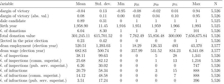
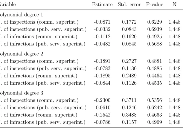
The second article is co-authored with Nezih Guner and Cezar Santos. We start by motivating with the fact that a large number of laborers in developing countries encounter poor working conditions. Corruption episodes related to labor inspections, some involving political figures, occur regularly in such environments. We investigate the effects federal deputy electoral results on labor inspections in firms that donate to electoral campaigns in Brazil from 2002 to 2014. To estimate a causal effect of electoral results on inspections, we use a regression discontinuity approach in close elections. We find no causal evidence that federal deputy electoral results affect variables related to labor inspections. This result is unchanged when we estimate heterogeneous effects as a function of labor inspection authorities’ position type, depending on which inspections can potentially be more or less influenced by political forces.
Lastly, the third paper is co-authored with Pedro Cavalcanti Ferreira and Cezar Santos. We provide a new education quality index for states within a developing country using 2010 Brazilian data. This measure is constructed based on the notion that the financial returns obtained from an additional year of schooling can be seen as being derived from the value that market forces assign to this education. We use migrant data to estimate returns to schooling of individuals who studied in different states but who work in the same labor market. We find very heterogeneous educational qualities. In fact, Brazil displays cross-state educational quality variation almost as large as that observed across countries. We compare our index with standardized test scores, educational outcome variables, and public expenditure per schooling stage at the state level, producing new evidence related to education in a large developing country. We conduct an education quality-adjusted development accounting exercise
for Brazilian states and find that human capital accounts for 26%-31% of output per worker differences. Adjusting for quality increases human capital’s explanatory power by 60%.
The Allocation of Public Expenditures Across
Educational Stages: A Quantitative Analysis for a
Developing Country
∗
Luiz Mário Brotherhood
Bruno Ricardo Delalibera
Brazilian School of Economics and Finance (EPGE/FGV)
May 8, 2018
Abstract
In this paper we study the allocation of public expenditures across educational stages in a developing country. We construct a general equilibrium model that features heterogeneous agents, credit restrictions, basic and tertiary education, public and private educational institutions. We calibrate the model’s parame-ters using Brazilian data. Simulations show three of the model’s features. First, economic inequality is mainly explained through endogenous educational deci-sions, instead of exogenous ability shocks. Second, abolishing public educational institutions contracts GDP by 5.5%, decreases welfare of households in the first income quartile by 7%, and does not affect significantly the welfare of the remain-ing households. Third, borrowremain-ing constraints are tight for the poorest agents in the economy. In the main exercise, we find that reallocating public expenditures from tertiary towards basic education to mimic Denmark’s allocation of public expenditures across educational stages decreases GDP, aggregate welfare and the Gini coefficient by 1.5%, 0.2% and 2%, respectively.
Keywords: education, educational stages, public expenditures, general equi-librium, development.
JEL Classification: I24, I25, I28, C68.
∗We thank Cezar Santos, Nezih Guner, Tiago Cavalcanti and Flávio Cunha for their comments and
1 Introduction
Governments all around the world use educational policies with the goal of increas-ing economic development.1 Educational stages are an important mechanism through
which educational policies affects development for, at least, two reasons: first, educa-tional investments in different stages produce distinct human capital outcomes at the individual–level;2 second, a different part of the population may be affected by an
ed-ucational policy depending on which eded-ucational stage it is focused on.3 In this paper,
we study the allocation of public expenditures across educational stages in a developing country.
Countries with similar development levels allocate public expenditures across edu-cational stages differently. Figure 1 displays cross-country data to support this claim. The horizontal axis exhibits log GDP per capita, and the vertical axis shows the ratio between public expenditures per student in basic (primary and secondary) and tertiary education (we call this variable “basic–tertiary expenditure ratio”), which we use as a measure of how governments allocate expenditures across educational stages. Mexico and Chile are developing countries with similar levels of GDP per capita that have very distinct basic–tertiary expenditure ratios. For each dollar that the Mexican (Chilean) government spends in a college student, 35 cents of dollar (1.06 dollars) are invested in a basic education student. On the other hand, the United States and Norway are examples of developed countries that use distinct educational policies. Basic–tertiary expenditure ratio is 0.97 in the US and 0.51 in Norway.
Discussing reasons why countries with similar development levels may allocate public educational expenditures differently introduces some of the ideas that will be present throughout this paper. First, governments may have different objectives when designing educational policies, such as increasing GDP per capita, fighting economic inequality or increasing welfare. Different goals may lead to different policy recommendations.4
A second reason why we may observe heterogeneity in countries’ allocation of public expenditures across educational stages is that, depending on a country’s economic en-vironment, each mechanism through which public policy affects economic development may have different relevance. Next, we discuss four of such mechanisms that are present
1In 2012, 4.7% of world GDP was spent by governments for educational purposes (World Bank,
2018).
2Heckman(2006) shows that early educational interventions produce higher human capital returns
than later interventions.
3In Latin American countries, rich students typically attend private schools while poor have to
resort to the lower quality public system (Menezes-Filho et al.,2014). In the United States, the top
two family income quartiles accounted for 77% of the bachelor’s degrees attained in 2014 (Cahalan
et al.,2016). For the case of Brazil, mean household per capita income of students in private schools are 2.54 higher than for public school students. Public college students are in households with per capita income 70% higher than households without college students (2002 National Household Survey Data).
4For papers on endogenous determination of public educational expenditures, see Su(2006) and
Figure 1: Basic–tertiary expenditure ratio and GDP per capita across countries
BDICAFBFABENCIV BWA CMR
COG CPV ETH GIN LSOGHA
MAR MDGMLI MOZ MRT MUS NAM NERRWA TCDSENSTP SWZ TGO TUN UGA BGD BRN BTN HKG IDN IND IRN ISR JPN KHM KOR KWT LAO LKA MAC MNG MYS NPL OMN PAK PHL SGP THA ALB ARM AUT BEL BGR CHE CYP CZE DNK ESP EST FIN FRA GBR GEO HUN IRL ISL ITA LTU LVA MDA MLT NLD NOR POL PRT SRB SVK SVN SWE UKRBLZ BRB CRI GTM JAM LCA MEX PAN USA AUS FJI NZL BOL BRA CHL COL ECU PER PRY URY 0 .5 1 1.5 2 2.5
Basic-tertiary expenditure ratio
6 8 10 12
Log GDP per capita Africa Asia Europe North America Oceania South America
Data sources: GDP per capita (Penn World Tables 8.1,Feenstra et al.,2015); government expenditure
per student (UNESCO, 2017).
Notes: Basic–tertiary expenditure ratio is the ratio between public expenditures per student in basic and tertiary education. Variables in both axes are means across 1999-2011 by country.
in this paper.
1. Public and private educational institutions’ relative efficiency. For a given edu-cational stage, public services’ relative quality vary across countries. The higher it is the ratio between public services’ relative quality (with respect to private services) for two educational stages, say a and b, all else equal, more resources should be allocated to a, in relation to b. For example, suppose that in a given country public universities’ quality is comparable to private universities’, but pub-lic schools are inferior to private schools. It may be optimal for the government to focus on tertiary education, leaving basic education for the private sector.5
2. Students sorting across public and private services. Governments finance them-selves using taxes in order to provide free schools and a limited number of spots in public colleges. Poor families choose to send their children to public schools in order to save on educational expenditures and have higher consumption. If government’s objective is to fight inequality, then a higher proportion of expen-ditures should be directed to public schools the greater it is the fraction of poor families, all else equal. On the other side, college admissions’ objective is to select the most well prepared students. If government’s objective is to increase GDP,
5We abstract from issues related with market power in educational markets. Private educational
maybe investments should be directed to high ability students through public college expenditures.
3. Credit restrictions in educational markets. In an environment with large credit frictions in educational markets, there may be individuals unable to fully explore their human capital potential. For example, a low income parent with a high ability child may not be able to invest optimally in her offspring’s basic education. In such cases, reallocating public expenditures from tertiary to basic education may be desirable.
4. Intergenerational transmission of human capital. Several forces affect the corre-lation between a parent’s and her offspring’s human capital. For example, in an environment where families have a big role in children’s moral formation, this cor-relation is higher than it would be in the case where families leave such issues to public educational services. On one hand, a strong intergenerational transmission of human capital can perpetuate inequality, where parents with low (high) human capital have children with low (high) human capital. A strong intergenerational persistence of human capital produces a high inequality of potential human cap-ital between students of public and private schools, reinforcing mechanism 2. On the other hand, a weak intergenerational persistence of human capital may gener-ate a high proportion of low income parents with high ability children, reinforcing mechanism 3.
In this paper, we construct a general equilibrium model that contains this mecha-nisms. The model features heterogeneous agents, credit restrictions, basic and tertiary education, public and private educational institutions.
Next, we discuss some aspects of the model in more detail. Households are repre-sented by overlapping generations. Each agent lives for four periods as a young child, old child, young parent and old parent. A child is born with a given level of innate ability independently drawn from a probability distribution. A young parent decides to send her child whether to a public or private school, which differ in two aspects. First, the marginal human capital returns of educational investments are different for the two types of schools, reflecting heterogeneous qualities. Second, each student in public school receives educational investment from the government through public ex-penditures.
A child’s acquired ability is her human capital in the stage after completing basic education. It is determined by her innate ability, basic educational investments and her parents’ human capital. To further improve future labor earnings, older children can attend college to increase human capital. Public and private colleges differ in the same aspects as schools, with one additional distinction: public college has a limited number of spots and admits students based on a noisy measure of applicants’ acquired ability, while vacancies in private colleges are unlimited. A grade point cutoff is determined
in equilibrium to make the mass of students entering public college consistent with the mass of vacancies supplied by the government. An agent’s human capital is interpreted as her labor productivity, and is determined by her acquired ability and educational investments in college.
There are no credit markets between periods, so that agents can not borrow against future earnings in order to invest in education and improve their children’s human capital.
We calibrate the model to fit Brazilian data related to educational choices and the labor market. The model is able to reproduce important statistics that were not used as targets in the calibration strategy. We then conduct some simple counterfactual exercises to understand some objects in the model. First, we show that our model explains economic inequality mainly through endogenous educational decisions, instead of through exogenous ability shocks. This is an important feature since we want to study educational policies. Second, government plays an important role in the model. We show that abolishing public educational services contracts GDP by 5.5%. It also decreases the welfare of households in the first income quartile by 7%, while, for the remaining agents, welfare barely changes. Third, we show that borrowing constraints to basic educational investments are tight for some agents in the economy. Basic edu-cational investments of poor households respond significantly more than of rich agents after an uniform lump-sum transfer to all households in the economy.
In our main counterfactual exercise, we find that GDP, aggregate welfare and the Gini coefficient are decreasing functions of basic–tertiary expenditure ratio. Simula-tions show that increasing Brazil’s basic–tertiary expenditure ratio by 80%, reaching Denmark’s level, decreases GDP, aggregate welfare and the Gini coefficient by 1.5%, 0.2% and 2%, respectively.
This paper is closely related to the hierarchical education literature (Lloyd-Ellis,
2000; Driskill and Horowitz, 2002; Su, 2004; Blankenau et al., 2007; Arcalean and Schiopu,2010;Abington and Blankenau, 2013).6 Papers in this literature were the first
to study the implications of human capital stages’ relevance to macroeconomic educa-tional policies. Specifically, these papers compare the economic consequences produced by different allocations of public expenditures across human capital stages, keeping total educational expenses (or its proportion w.r.t. GDP) constant. However, most papers in this literature are theoretical and focus on stylized models that are inappropriate for answering applied questions. Arcalean and Schiopu (2010) is the only quantita-tive paper in this branch of literature that we are aware of. These authors calibrate an equilibrium model to match data on education finance in the OECD countries to study the growth maximizing allocation of public resources. These authors’ main focus is on how parameters of the human capital production function determine outcomes of educational policies, and how households react to such policies in terms of
tional expenditures. They find that the growth maximizing share of public spending devoted to basic education in the OECD countries should be high. We contribute to this literature by building and calibrating a rich model that encompasses several rele-vant features not considered by previous papers, such as heterogeneous agents, credit restrictions, and differences between public and private educational institutions.
We also contribute to the literature that studies market failures in education markets (Lochner and Monge-Naranjo, 2011; Cunha, 2013; Caucutt and Lochner, 2017) by analyzing how these distortions work as mechanisms in the trade-off between public investments in basic and tertiary education. Our results point that credit restrictions play a big role in the model.
This paper is composed of four more sections. Section 2describes the main model. Section 3 presents the calibration and discusses the benchmark economy. Section 4
discusses counterfactual exercises. Section 5 discusses next steps that we will follow to advance this research project. Appendix A presents a simple version of the model, which allows us to analyze in a clear way some mechanisms present in the complete model. Appendix B contains mathematical proofs.
2 Model
The model is based onRestuccia and Urrutia(2004) andHerskovic and Ramos(2017).7
It is composed of households, a representative firm that produces the final good, and the government. Households are represented by overlapping generations that make decisions on consumption and education, and supply human capital to the final good firm. The final good firm employs human capital and produces the consumption good. The government taxes households and provides educational services for free. There are two levels of education (basic and tertiary), and two types of education (private and public).
Households Each agent lives four periods, the first two as a child (young and old
child) and the other two periods as an adult (young and old parent). Each generation is a continuum of positive measure, and a family unit comprises one parent and one child. At each point in time, there are two different family units: one with a young child and a young parent, and another with an old child and an old parent. Each period in the model is interpreted as a 18–years period. There is no population growth. Agents are heterogeneous in their innate ability levels; a young child is born with a stochastic innate ability level. Decisions are made at the family level – parents make consumption and educational investment choices, maximizing the welfare of the family. Furthermore, households have access to a perfect credit market within period, but no credit market
7Throughout this section, we borrow descriptions of some objects of the model fromHerskovic and
between periods.
Human capital A child’s human capital is determined by three types of variables:
innate ability, effective educational investment, and her parent’s human capital. Effec-tive educational investment is determined by educational investment, which represents monetary expenditures in educational goods and services, such as schools, books, etc. The transformation of educational investment into effective educational investment de-pends on whether a public or a private educational institution is chosen.
Young households make decisions related to basic education. A young household chooses an education type, sy ∈ {1, 2}, where sy = 1 denotes private school and sy = 2
denotes public school, and an education expenditure in school ey ≥ 0.8 Effective basic
educational investment ˆey is determined by
ˆey(sy, ey) = ey if sy = 1 (private school) αy(gy + ey) if sy = 2 (public school), (1) where αy > 0 captures the quality difference between public and private schools, and
gy ≥ 0 is public expenditure per student in public school.
Old households make decisions related to college education. An old household de-cides between having no college, so = 0, private college, so = 1, or public college,
so = 2. This decision, together with the education expenditure in college eo ≥ 0, pins
down effective college investment ˆeo through
ˆeo(so, eo) = 0 if so = 0 (no college) eo if so = 1 (private college) αo(go+ eo) if so = 2 (public college). (2) Parameter αo > 0 captures the quality difference between public and private colleges,
and go ≥ 0 is public expenditure per student in public college.
The acquired ability of an individual, ˆπ, is defined as the human capital that she has in the stage immediately after completing basic education. It is determined by the agent’s innate ability π, her parents’ human capital h, and basic educational investment ˆey, through a constant elasticity of substitution (CES) technology:
ˆπ(π, h, ˆey) = π h
γyhφy + (1 − γy)ˆeφyy i1/φy
, (3)
where 0 ≤ γy ≤ 1 is a parameter that measures parent’s human capital relative
im-portance to acquired ability formation, and φy ≤ 1 drives the elasticity of substitution
between h and ˆey.
8We posit that young children cannot work. In the 2002 Brazilian National Household Survey
The human capital of an individual is determined by her acquired ability ˆπ, and effective educational investment in college education ˆeo:
h0(ˆπ, ˆeo) = h
γoˆπφo + (1 − γo) (ψ + ˆeo)φo iθ/φo
, (4)
where 0 ≤ γo ≤ 1, and φo ≤ 1 have similar interpretations as in (3), 0 < θ < 1 measures
the degree of decreasing returns to scale, and ψ > 0 drives the marginal return of tertiary education effective investment for an individual without college. Note that, if ψ = 0, (4) is a standard CES production function with INADA conditions. We make ψ > 0 because this specification leads to positive human capital in the case where the individual does not study in college, that is, ˆeo = 0.
Young households The state variable of a young household is given by the parent’s
human capital h and the child’s innate ability π. The parent inelastically supplies human capital services in the labor market and her labor income is equal to wh, where w is the equilibrium wage rate. The government proportionally taxes labor income at rate τ. The young parent chooses its child’s education type, sy, and decides how
to allocate her after-tax labor income between consumption, cy, and basic education
expenditures, ey. Thus, the problem of a young parent is given by
Vy(h, π) = max cy≥0 sy∈{1,2} ey≥0 u(cy) + βVo(h, ˆπ(π, h, sy, ey)) s. t. cy+ ey = (1 − τ)wh ˆπ(π, h, sy, ey) = π h γyhφy + (1 − γy)ˆey(sy, ey)φy i1/φy . (5)
The function Vy(·) is the value function of the young parent, u(·) is the utility function
of the family, and β is a time discounting parameter. The function Vo(·) is the value
function of the old parent. We assume no credit market between periods: all young parents’ earnings are either consumed or invested in basic education. However, since each period represents 18 years, the budget constraint implies a perfect credit market within-period.9
9The private education technology in this model can be interpreted as educational firms with
constant returns to scale and constant marginal cost operating in a competitive market. To see this, suppose that there is a continuum of private schools indexed by their quality, q ≥ 0. A firm’s quality is the effective educational investment it provides to their students, that is, q = ˆe. The problem of a representative firm with a given quality q is to choose the number of vacancies to supply, µ, taking as given its price, p, to maximize profits, pµ − cµ, where c is the firm’s constant marginal cost, given by
c= q. The equilibrium conditions in those markets are p(q) = q for each q ≥ 0. If a household chooses
Old households An old parent chooses how to allocate her family labor income
between consumption and investment in college education. Specifically, an old parent chooses whether or not to have her child apply to college, and, therefore, her value function is defined as
Vo(h, ˆπ) = max{Vonot apply(h, ˆπ), Voapply(h, ˆπ)}, (6)
where Vnot apply
o (·) is the value of not applying, and Voapply(·) is the expected value of
applying to college.
If a child does not apply to college, then she immediately joins the labor market, inelastically supplying her human capital services. Thus, under no college education, the value of not applying is
Vonot apply(h, ˆπ) = u(co) + βEπ0[Vy(h0(ˆπ, 0, 0), π0)]
s. t. co = (1 − τ) [wκξ1h+ wξ2h0(ˆπ, 0, 0)] h0(ˆπ, so, eo) = h γoˆπφo + (1 − γo) (ψ + ˆeo(so, eo))φo i1/φo . (7)
The budget constraint includes the post-tax income from all family members combined. ξ1 >1 and ξ2 <1 are life-cycle earnings parameters that measure, respectively, by how
much old adults are more productive than young adults, and how much old children are less productive than young adults. Parameter κ represents the fraction of the time period that old adults work. Since in this case the old child does not study in college, all income goes to consumption. The continuation value of the old parent is the expected value function of her own child as a young parent in the next period. This expectation is over the innate ability distribution of the old parent’s grandchild, which follows an i.i.d. log-normal distribution,
log(π0) ∼ N(0, σ2
π). (8)
To enter both public or private college, children must apply. We assume that all college applicants are automatically admitted to private college.10 The same is not true
for public college. The outcome of an application to public college is random. The probability of admission depends on applicants’ acquired ability, and college applicants
educational investment ˆe = q. Summing up, in this modification we only add firms as intermediates between households and the effective educational investment technology. Although simple, this is useful to think about our model in terms of several issues, such as, for example, how it is related with papers in the Industrial Organization literature that model educational markets in more sophisticated ways (see, for example,Sanchez(2017)).
10AsHerskovic and Ramos(2017) describe, according to 2008 Brazilian data, there are nearly seven
times more students applying to public college than public college spots available. However, for a private college, the ratio of applicants to private college spots is about 1.3. Moreover, only 5% of the public college spots are unfilled, while 50% of the private college spots are unfilled.
with higher acquired ability are more likely to be admitted. Probability of admission is given by q(ˆπ), and it is an equilibrium object that we discuss later in this section, along with a description of the college admission market. Taking the probability function as given, the expected value of applying to college is a combination of the value if admitted Voadmitted(·) and the value if not admitted Vonot admitted(·):
Voapply(h, ˆπ) = q(ˆπ)Voadmitted(h, ˆπ) + [1 − q(ˆπ)]Vonot admitted(h, ˆπ). (9) If an old child’s college application is successful, the old parent value function is described as Voadmitted(h, ˆπ) = max co≥0 so∈{1,2} eo≥0 u(co) + βEπ0[Vy(h0(ˆπ, so, eo), π0)] s. t. co+ eo= (1 − τ) [wκξ1h+ wξ2h0(ˆπ, so, eo)(1 − η)] h0(ˆπ, so, eo) = h γoˆπφo + (1 − γo) (ψ + ˆeo(so, eo))φo i1/φo . (10)
Admitted households choose between public and private colleges. Parameter η captures the time spent in college. This represents the opportunity cost associated with a college education since the old child can work only a fraction 1 − η of that period.
If an old child is not admitted to a public college, then she may still attend a private college. Conditional on the child not being admitted to the public college, an old parent chooses between enrolling her child in private college (so = 1) or not (so = 0). The
old parent’s optimization problem if her child is not admitted to a public college is, therefore, given by
Vonot admitted(h, ˆπ) = max
co≥0 so∈{0,1} eo≥0 u(co) + βEπ0[Vy(h0(ˆπ, so, eo), π0)] s. t. co+ eo = (1 − τ) [wκξ1h+ wξ2h0(ˆπ, so, eo)(1 − ηso)] h0(ˆπ, so, eo) = h γoˆπφo + (1 − γo) (ψ + ˆeo(so, eo))φo i1/φo . (11)
Public college admissions We model public college admissions as a competitive
market in which applicants compete for college spots. As the result of an old child’s application, the college observes a noisy signal of her ability. This signal is interpreted
as her application score or her grade on the admission exam, and it is determined by log(ˆπobserved) = log(ˆπ) + σ
pεp, (12)
where εpis an i.i.d. standard normal, and σpis the noisiness of admissions. The measure
of potential applicants is one, which includes all old children, while the measure of spots available at the public college is given by parameter µ. Given the number of college spots available, public college admits applicants with the highest score until all spots are filled, or until there is no more demand for spots. There is a grade point cutoff, π∗, such that every applicant with ˆπobserved ≥ π∗ is admitted. The cutoff π∗ is the
equilibrium variable that clears the admissions market. Denote by νo the mass of old
children that are admitted and choose to study in public college. The condition for admissions market clearing is:
π∗(µ − νo) ≥ 0, with equality if π∗ >0, (13)
that is, if the grade point cutoff is strictly positive, then all spots must be filled. How-ever, it is also possible the case where the grade point cutoff is zero and there are empty slots in equilibrium.
Firm The representative final good firm takes the wage rate w as given and has a
constant returns to scale production technology. The problem of the firm is max
H≥0 AH− wH, (14)
where A is total factor productivity and H is aggregate human capital. Denote by H∗
the optimal choice of the firm. The product in the economy is Y = AH.
Government The government offers public education and finances itself by taxing
households. For each student in public school and college, the government spends gyand
go, respectively. Denote by νy and νo the equilibrium mass of households that study
in public school and public college. The condition for government’s budget balance requires expenditures to be equal to revenues:
(0.5)gyνy+ (0.5)goνo = τY. (15)
Public spending per student in college education go is an equilibrium variable, while
the ratio of public spending per student in the two educational stages gy/go and the
tax rate τ are parameters.
Equilibrium A Stationary Recursive Competitive Equilibrium in this economy is
spending per student in public college go, grade point cutoff π∗, distributions of young
and old households across state variables, such that:
1. Value and policy functions solve households’ functional equations. 2. Labor demand solves the final good firm’s problem.
3. Final good market clears:
Y = Cy+ Co+ Ey+ Eo+ G, (16)
where Cy and Co are the aggregate consumption of young and old households, Ey
and Eo denote total private spending in education of young and old households,
and G = τY is government’s total expenditure in public education.
4. Labor market clears: firm’s optimal labor demand is equal to the aggregate human capital supplied by households.
5. The mass of public college students is less than or equal to the mass of public college vacancies, with equality if π∗ >0.
6. Government’s budget is balanced.
7. The distribution of young and old households is stationary and consistent with households’ policy functions.
3 Calibration
We calibrate the model using Brazilian data. We interpret each period of the model as consisting of 18 years. This implies that young children are 0 to 17 years old, old children are 18 to 35, young adults are 36 to 53, and old adults are 54 to 71. We split the set of parameters in two: in the first subset, parameter values can be directly obtained from the data or borrowed from the literature. Parameters in the second subset are estimated through the Simulated Method of Moments.
Table 1 displays values for parameters in the first set. We assume that agents have constant relative risk aversion (CRRA) preferences, u(c) = c1−σ−1
1−σ , with a risk
aversion of σ. We calibrate this parameter at 1.5, which is a reasonable parameter value considering several estimates from the literature. The discount is calibrated at 0.96 per year.
To estimate κ, we use 2002 Brazilian National Household Survey (PNAD)11
cross-section data and find that 60 years is the smallest age value such that the majority
11We use 2002 data to calibrate the model because a big government program that concedes
schol-arships for low-income individuals to study in private universities (ProUni) was implemented in 2004. Since we do not model this program, we decide to use data prior to its implementation.
of individuals do not work. Therefore, we posit that old adults stop working when they reach 60 years, implying that those agents work for 7/18 of the period in the model. We use 2002 PNAD data to estimate life-cycle parameters ξ1 and ξ2 following
a strategy similar to Restuccia and Urrutia’s (2004): we compare mean earnings of college-educated individuals in the age intervals of old children, young and old adults. We find that college-educated old children (old adults) mean earnings are equal to 70% (128%) of those of young adults.
In 2002, 11% of 18 to 35 year-old individuals were either college students or had completed college. Out of all 18 to 35 year-old college students, 25% were enrolled in public college. Thus, the measure of public spots is calibrated at µ = 0.028, which is 25% of 0.11.
In 2002, public expenditures in education (primary, secondary and tertiary) as a proportion of GDP were equal to 3.5% in Brazil (UNESCO, 2017). We use this value for τ. In yearly terms, the ratio between public spending per student in basic education and college is 0.22. To calibrate gy/go, we multiply this number by 12/5 to account for
the fact that the duration of basic education equals 12 years, while students usually take 5 years to complete an undergraduate course in university.
Values for the remaining parameters in the model are not directly observable in the data or cannot be borrowed from the literature. Therefore, we use the Simulated Method of Moments and choose parameter values such that the model produces statis-tics related to educational choices and the labor market that are close to the ones observed in Brazil.
We calibrate eleven parameters. There are eight parameters related to the human capital function: relative efficiencies of public education, αy and αo, relative importance
of inputs, γy and γo, elasticity of substitution drivers, φy and φo, marginal return to
college educational investment, ψ, and a return to scale parameter, θ. We also calibrate innate ability dispersion, σπ, public college admission process noisiness, σp, and fraction
of time spent in college, η.
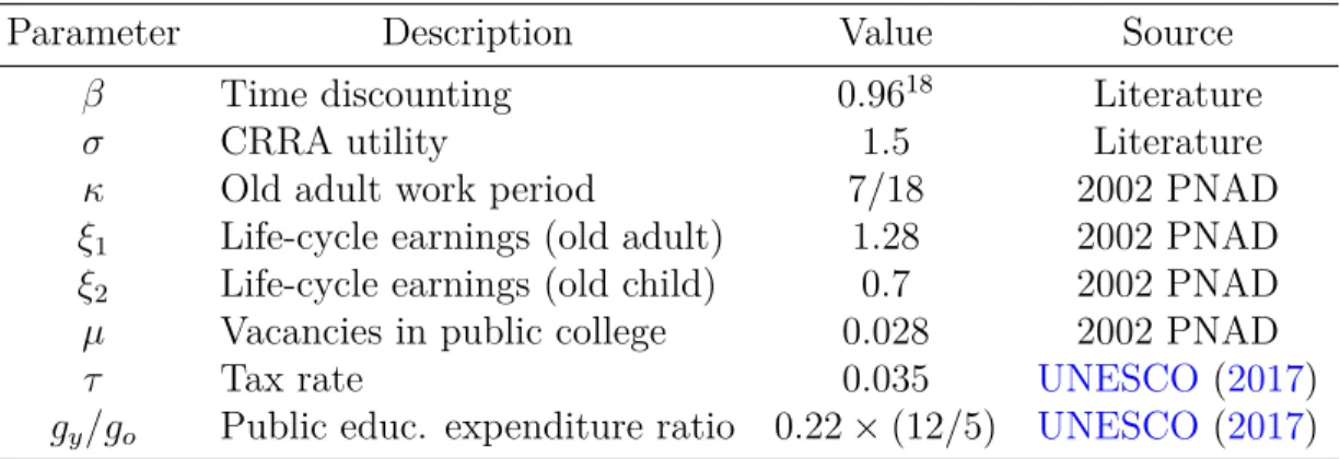
Table 1: Externally calibrated parameters
Parameter Description Value Source
β Time discounting 0.9618 Literature
σ CRRA utility 1.5 Literature
κ Old adult work period 7/18 2002 PNAD
ξ1 Life-cycle earnings (old adult) 1.28 2002 PNAD
ξ2 Life-cycle earnings (old child) 0.7 2002 PNAD
µ Vacancies in public college 0.028 2002 PNAD
τ Tax rate 0.035 UNESCO (2017)
We select nine moments in the data to match:12 two related to labor earnings
(dispersion and intergenerational correlation13); four related to discrete educational
choices (fraction of students in private schools, proportion of individuals without college education and with private tertiary education, and fraction of applicants to public college); two related to continuous educational choices (fraction of GDP spent in school and tertiary education by households); and one related to educational returns (college wage premium).
Table2displays parameter values that we obtain when using the Simulated Method of Moments, and Table 3 compares statistics in the data and model. Out of the nine moments, there are two that display large errors: standard deviation of log earnings (error = −52%) and fraction of applicants (error = −26%). However, we show next that the model reproduces well the earnings percentiles in the data, revealing that the error related to earnings dispersion is not a major issue.
Non-targeted moments Next we discuss the model’s performance in fitting
statis-tics that were not targeted in the calibration process. Figure 2 shows ratios between percentiles of the earnings distributions in the model and in Brazilian data. We com-pare the 90th earnings percentile with percentiles 10, 25, 50 and 75, obtaining relative errors equal to -6.7%, 22%, 42% and -9.9%, respectively. Given that such statistics were not targeted in the calibration procedure, we consider the fit to be good.
Table4shows choices related to basic education by households’ income quartiles. In the model, all parents in the first two quartiles choose to send their children to public schools, which is approximately what we see in the data. For the third quartile, there
Table 2: Internally calibrated parameters
Parameter Description Value
σπ Innate ability AR innovation variance 2.3762
σp Noisiness of admission process 3.7968
αy Public school relative efficiency 0.5739
αo Public college relative efficiency 0.9796
γy Human capital share parameter (young child) 0.1757
γo Human capital share parameter (old child) 0.9281
φy Elasticity of substitution (young child) -2.9748
φo Elasticity of substitution (old child) -0.9308
ψ Marginal return of college investment 0.1121 θ Human capital returns to scale 0.3841
η Time spent in college 0.7726
12Currently this is an underidentified model. In the future we plan to add more moments to conduct
an exactly identified calibration.
13Intergenerational correlation of earnings is defined as the regression coefficient obtained by
Table 3: Data and model comparison
Moment Source Data Model
Standard deviation of log earnings 2002 PNAD 0.9906 0.4744
Intergenerational correlation of earnings Dunn(2007) 0.6900 0.5824 Fraction of applicants Herskovic and Ramos (2017) 0.2560 0.1894
Young children in private school 2002 PNAD 0.1236 0.1074
Old children without college 2002 PNAD 0.8924 0.8961
Old children in private college 2002 PNAD 0.0789 0.0752
Fraction of GDP spent in school by households Herskovic and Ramos (2017) 0.0260 0.0211 Fraction of GDP spent in college by households Herskovic and Ramos (2017) 0.0080 0.0099
College wage premium 2002 PNAD 3.2851 3.0753
Figure 2: Earnings distribution percentile ratios
are no children in private schools in the model, but there is 12% in the data. The model fits well basic educational choices in the top quartile.
Table 5shows that the model is able to reproduce the pattern of tertiary education choices by earnings quartiles. In the simulation, all private college students are in the top earnings quartile.
Benchmark model analysis Since we have calibrated parameters, we can now study
some of the model’s objects. Next, we study the human capital production function (3) and (4). Its functional form does not follow a standard CES specification, so that it does not display constant elasticity of substitution between educational expenditures in basic and tertiary education. Figure 3 shows an isoquant associated with a private college student with median h and ˆπ, supposing that this student goes to private school when young. Dotted lines show the points in the curves where this student is located. The elasticity of substitution between inputs in basic and tertiary education is an increasing function of the Marginal Rate of Technical Substitution (MRTS). That is, as the MRTS increases and we move from right to left along the isoquant, the two inputs become more complementary. For the case of this student, since the elasticity of substitution is smaller than one, investments in basic and college education are complementary inputs of the human capital production function. This result is in line with the literature on human capital formation (Cunha et al., 2006), which finds that inputs in different educational stages are complementary.
Table 4: Basic education choices by earnings quartiles
Data Model
Private Public Private Public
Q1 1.54 98.46 0 100
Q2 4.73 95.27 0 100
Q3 11.97 88.03 0 100
Q4 47.85 52.15 44.73 55.27
Table 5: Tertiary education choices by earnings quartiles
Data Model
No college Private Public No college Private Public
Q1 98.52 0.98 0.49 100 0 0
Q2 95.98 2.81 1.22 98.94 0 1.06
Q3 90.83 6.62 2.55 98.92 0 1.08
Q4 68.69 23.93 7.38 59.79 31.28 8.93
Data source: 2002 PNAD.
Figure 3: Human capital production function
4 Counterfactuals
In this section we present counterfactual exercises with the objective of studying the cal-ibrated model and answering our main research question, which looks for the economic effects of reallocating public expenditures across educational stages.
Educational choices and economic inequality We start by investigating the
model’s capacity of explaining economic inequality through endogenous educational choices. We compute earnings’ stationary distributions in two counterfactual cases. First, we suppose that agents make homogeneous educational decisions (all agents go to public schools, spend zero in education, and do not apply to college), but innate ability distribution is the same as in the benchmark case. In the second exercise, we posit that all agents have the same innate ability (equal to benchmark mean innate ability), but make the same educational choices as those in the baseline model. Note that, in those counterfactual scenarios, agents do not behave optimally. Our objective here is to conduct a simple decomposition of economic inequality into two variables (educational choices and innate abilities).
We find that, in the first exercise, the Gini coefficient decreases by 64%, while, in the second case, it decreases by 29%. The fact that inequality decreases by a larger amount in the first case shows that educational decisions are more important than innate ability heterogeneity to explain earnings inequality in the model. If we additionally use relative Gini variations produced in the two exercises as a measure of the importance of a given feature in explaining inequality, we conclude that educational choices are about (64%)/(29%) = 2.2 times more important than innate abilities to explain earnings heterogeneity. This result suggests that educational policies can have large impacts on economic inequality in the model.
Explaining intergenerational correlation of earnings We can also conduct an
exercise similar to the previous one to evaluate how the intergenerational correlation of earnings is generated in the model by two mechanisms: parent–child direct human capital transmission, through parameter γy, and educational decisions. We again run
two counterfactuals. First, we make γy = 0 and use benchmark educational decisions.
Second, we use the baseline value for γy but suppose that agents make homogeneous
educational decisions (same as those in the previous exercise). We find that intergen-erational correlation of earnings decrease by 87% in the first case and by 99% in the second case. The fact that intergenerational correlation of earnings decrease by a large amount in both experiments shows that the two mechanisms are crucial to explain it.
The role of government in the economy Next, we study the role of public
edu-cational services by computing the equilibrium for the case in which there is no gov-ernment. Specifically, we make τ = π∗ = g
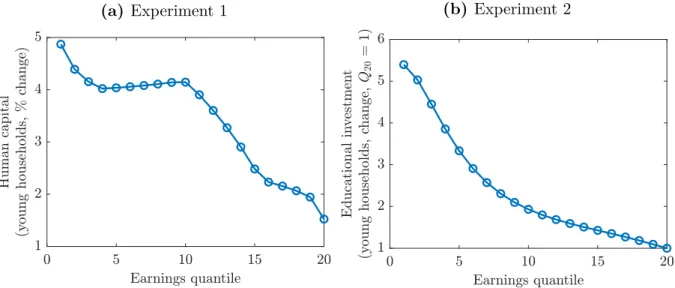
Figure 4: Credit frictions evaluation experiments
(a) Experiment 1 (b) Experiment 2
which includes finding agents’ optimal choices. Comparing the benchmark and counter-factual stationary equilibria, we find that GDP decreases by 5.5%, the Gini coefficient decreases by 0.16% and aggregate welfare14decreases by 1.89%. Impacts on welfare are
heterogeneous with respect to households’ earnings: lifetime utility of poorest house-holds in the first earnings quartile decrease by 7%, while welfare for househouse-holds in the second, third and fourth quartiles vary by 0.7%, -0.36% and -1.2%, respectively. We conclude that government plays an important role in the model, increasing the utility of poor households in the economy.
Credit frictions To evaluate the strength of credit constraints in the model, we
first investigate returns to basic educational investments for different agents in the benchmark economy. For the same level of basic educational investment, an average poor student has a lower human capital return to investments in basic education than a rich child. This happens because of three reasons: poor parents transmit a lower human capital to their child, public schools provide a lower human capital return to expenditures than private schools, and rich parents have higher effective educational investments in tertiary education. However, since households do not invest equally, educational returns in the benchmark equilibrium may display a very different pattern from the case of homogeneous basic educational investments.
To compute educational returns, we add a lump-sum basic educational expenditure equal to half the mean earnings of young households in the first quartile to all young children and keep everything else constant. Figure 4a shows the effects of this exper-iment on the human capital change of children for 20 quantiles of parents’ earnings. Despite the reasons discussed in the previous paragraph, poor children have higher
Figure 5: Counterfactual equilibrium values of gy and go
Note: x is a factor by which we multiply gy/go to get a counterfactual g0y/g0o= x (gy/go).
cational returns than rich students, showing that there is a significant mass of relatively productive poor students that receive small educational investments in school.
Next, we follow the intuition of experiments executed in Carneiro and Heckman
(2002) and Restuccia and Urrutia (2004) to study the strength of credit frictions in the model. We add a lump-sum income transfer to all households in the economy equal to the same amount of the previous exercise and recompute their optimal choices. If we consider that households in the top income quantiles are credit unrestricted, then the relative change in educational expenditures of a given household with respect to the richest households should gives us an idea on how much this household is constrained in terms of credit for educational investments. Figure 4b shows the change in basic educational investment by 20 quantiles of parents’ earnings, normalizing the largest quantile’s expenditure change to one. Young households in the first quartile increase educational spending by more than three times the spending increase of the top quar-tile. We conclude from this experiment that borrowing constraints to investments in education in our model do have an important impact on young parents’ decisions.
Relocation of public expenditures across educational stages Remember that
the ratio between public spending per student in basic and tertiary education, gy/go, is a
parameter in the model. Our main exercise consists in varying this ratio and studying counterfactual equilibria driven by different educational policies. Since we keep the tax rate τ fixed, varying gy/go is equivalent to reallocating public expenditures across
educational stages, keeping fixed the proportion of GDP spent in education by the government.
Figure 5 shows equilibrium values of gy and go for each counterfactual simulation.
Note that, to reallocate expenditures from tertiary to basic education, go needs to fall by
Figure 6: Reallocating public expenditures across educational stages
(a) GDP (b) Welfare
(c) Gini coefficient
Notes: Values in the horizontal axis are normalized so that baseline gy/gois equal to 1.
public expenditures in basic education is significantly bigger than the mass of students in public college. Finally, Figure 6 displays the results of the counterfactual exercise. Reallocating public expenditures from tertiary to basic education leads to lower GDP, lower aggregate welfare, and lower Gini coefficient. For the maximum reallocation that we simulate, GDP, welfare and the Gini coefficient decrease by 1.3%, 0.2% and 2%, respectively.
5 Next steps
There are several analysis that we plan to execute in the future to advance this research project. Next, we describe some of them. In subsection 5.1 we discuss in detail the
implementation of voucher payments for private schools in the model.
1. Fully investigate the main results. In this text, we analyze the impact of a realloca-tion of public expenditures across educarealloca-tional stages on macroeconomic variables (GDP, inequality and welfare). We can further study how different types of house-holds are affected by the policy. We find that aggregate welfare decreases, but it is possible that poorer households benefit from the policy. We can also study how agents react to the policy in terms of educational spending and applying to public college. Finally, we can decompose the counterfactual results using partial equilibrium analysis to understand, for example, how macroeconomic variables would have changed if households had not reacted to the policy. This would give us an idea on how much of the effects of the policy on macroeconomic variables are explained by households adjusting to the policy.
2. In our main exercise, we vary gy/go, keep τ fixed, and interpret this as a
realloca-tion of expenditures without changing the proporrealloca-tion of GDP spent in educarealloca-tion by the government. We can also think in reallocating expenditures across educa-tional stages, keeping fixed total expenditures in education. This can be done in two ways:
(a) First, for some g0
y/go0 different from gy/go, we look for a new tax rate τ0
such that τ0Y0 = τY , where Y0 is the equilibrium GDP associated to the
new variables with prime superscript. That is, we reallocate expenditures across educational stages and look for the tax rate that makes new total public expenditure equal to the baseline one. However, comparing the results of this exercise with the ones produced by the counterfactual described in Section4may be confusing, since varying τ affects households at the margin, potentially leading to large changes in households’ optimal choices. The experiment in the next item can be executed to decompose the differences between the two counterfactuals.
(b) We run the same counterfactual as the one described in Section 4, but we change the equilibrium definition by substituting government’s budget bal-ance condition by the restriction τY = τY0. That is, we reallocate
expendi-tures in a way that keeps total expendiexpendi-tures and the tax rate fixed. This is a partial equilibrium analysis in the sense that it ignores government’s budget balance condition.
3. We can make public educational expenditure be a function of parent’s earnings, gy(h) and go(h). Making this functions decreasing reallocates resources from rich
to poor agents. Through making expenditures negative for some households we can simulate a policy where, for example, rich households must pay a fixed cost to study in public college, with this money being reallocated to poor students in public schools or to voucher payments in private schools.
4. In our calibration, public schools have very low relative quality, αy = 0.57, which
is consistent with Brazilian data.15 We can assess the importance of this fact by
simulating counterfactual values for αy.
5. In 2004, a big government program that concedes scholarships for low-income individuals to study in private universities (ProUni) was implemented in Brazil. We can use this policy in two ways in our model. First, as part of the calibration strategy, we can make our model reproduce the short-run effects of this policy, as measured by econometric policy evaluation works.16 Second, we can estimate
the long-run effects of such policies by computing the new stationary equilibrium after the reform, possibly including the transition between the two steady states.
5.1 Vouchers for private schools
In this subsection we show how to implement a voucher policy for private schools in the model. We also show heuristically that increasing public expenditures for students in public schools attracts to the public system children with the smallest innate abilities in private schools. Additionally, this policy leads to a negative jump in the educational expenditures of agents that switch from private to public schools. We argue that the opposite happens for the case of voucher payments. This can potentially be an ad-vantage of voucher policies over public expenditures in public schools: voucher policy leads to a positive jump in the human capital of some students that otherwise would be the ones with the highest innate abilities in public schools. An important caveat: throughout this discussion we abstract from general equilibrium effects.
First, a voucher policy can be implemented in the model by supposing that the government pays a fixed amount per student in private institutions. This payment can be made conditional on parent’s earnings. Thus, suppose that the government invests vy(h) for each student in private school whose parent’s earnings are h. This modifies
the effective educational investment function (1) to be ˆey(sy, ey, h) = vy(h) + ey if sy = 1 (private school) αy(gy + ey) if sy = 2 (public school). (17) Next, we present some auxiliary arguments:
1. Expenditures if choosing a private school is higher than if choosing a public school. Inspecting the value function of a young household in equation (5), it is possible to see that, whether the household is choosing a public or private school, there is a one to one substitution between consumption and educational expenditure.
15Brazil has the lowest ratio between public and private math scores in PISA’s 2015 sample.
16This kind of structural model usage is in line with recent ideas discussed in Low and Meghir
This implies that, for a given level of educational expenditure, the marginal costs of increasing expenditures by one unit in the public and private schools are equal. The same is not true for the marginal human capital return of educational in-vestment. For a given point of basic educational investment, the human capital function is more concave in the case of public schools since αy <1, implying that
the marginal benefit of educational expenditures are bigger in private schools. These two facts imply that, for a given household, the optimal educational in-vestment if choosing a private schools is larger than if choosing a public school. 2. If gy increases, there is crowding-out of households’ educational expenditures.
Fix-ing a given level of educational expenditures of a household, if gy increases, by
concavity of the human capital function, the marginal human capital return of educational expenditures decreases. Since the marginal cost is kept fixed, this implies that optimal educational expenditures of households in public schools decrease when gy increases, e.g., there is crowding out of public educational
ex-penditures. A similar reasoning shows that households in private schools crowd out voucher payments.
3. Optimal educational expenditures are increasing in children’s innate ability. Take two young households with same h but with innate abilities π1 < π2. For the
same level of educational expenditures, the marginal human capital return driven by an increase of educational expenditures is greater for the household with π2,
implying that the marginal benefit of educational expenditures is greater for π2.
Together with the fact that marginal costs are equal for both households, this shows that the optimal educational investment is increasing in π.
4. Existence of innate ability threshold ˜π(h) that separates households choosing public and private schools. Figure 7 shows effective educational investment functions for the case of no voucher payments. Note that effective educational investment in private schools, ˆey(1, ey), is the identity function, while, in the public case,
ˆey(2, ey), it is a line with slope equal to αy, which is smaller than one, and positive
intercept equal to αygy. Define ˜ey as the point where the two lines cross each
other. Note that households that choose ey <˜ey in equilibrium must be choosing
public schools (otherwise they could spend the same amount in public schools and get a strictly greater ˆey), while households that spend ey > ˜ey go to private
schools. Together with the fact that, given h, optimal educational expenditure is increasing in π, this implies that there is a threshold ˜π(h) such that households with earnings h and π < ˜π(h) choose public schools and households with π > ˜π(h) choose private schools.
Abstracting from general equilibrium effects, when the government increases gy to
g0
Figure 7: Effective educational investment ey ˆey(1, ey) ˆey(2, ey) αygy ˜ey
education and choosing public school strictly increases. Thus, more students will choose public schools, moving up the ability threshold to ˜π0(h). That is, increasing g
y attracts
the students from private schools with the smallest innate abilities π such that ˜π(h) < π < ˜π0(h).
At the same time, since a household’s optimal educational expenditures are smaller in public schools than in private schools, students that switch to public schools discretely decrease their educational expenditures, leading to a negative jump in their human capital. The fact that households crowd out public expenditures when gy increases
makes this negative jump bigger.
On the other hand, if the government increases voucher payments in private schools, more households choose to study in private schools. This decreases the ability threshold from ˜π(h) to ˜π00(h). For a given h, households that switch to private schools are those
such that ˜π00(h) < π < ˜π(h).
The effect on educational expenditures for a given switching student is ambiguous in the case of an increase in voucher payments. On one hand, switching for private schools leads to a positive jump in the educational expenditure. On the other hand, an increase in voucher payment crowds out private investments. However, making the increase in voucher payments small enough should make the first effect larger than the second, since the first one is discontinuous and the second is smooth with respect to voucher payment changes.
References
Casey Abington and William Blankenau. Government education expenditures in early and late childhood. Journal of Economic Dynamics and Control, 37(4):854–874, 2013. URL http://EconPapers.repec.org/RePEc:eee:dyncon:v:37:y:2013:i: 4:p:854-874.
hierarchical education system. Journal of Economic Dynamics and Control, 34(4): 604–622, 2010. URL https://EconPapers.repec.org/RePEc:eee:dyncon:v:34: y:2010:i:4:p:604-622.
William Blankenau, Steven Cassou, and Beth Ingram. Allocating government education expenditures across k-12 and college education. Economic Theory, 31(1):85–112, 2007. URL https://EconPapers.repec.org/RePEc:spr:joecth:v:31:y:2007:i: 1:p:85-112.
Cahalan, Margaret, Perna, Laura, Yamashita, Mika, Ruiz, Roman, Franklin, and Khadish. Indicators of Higher Education Equity in the United States: 2016 Historical Trend Report. Pell Institute for the Study of Opportunity in Higher Education, Council for Opportunity in Education (COE) and Alliance for Higher Education and Democracy of the University of Pennsylvania (PennAHEAD), 2016. URL http: //www.pellinstitute.org/publications-Indicators_of_Higher_Education_ Equity_in_the_United_States_2016_Historical_Trend_Report.shtml.
Pedro Carneiro and James J. Heckman. The evidence on credit constraints in post-secondary schooling. The Economic Journal, 112(482):705–734, oct 2002. doi: 10. 1111/1468-0297.00075.
Elizabeth Caucutt and Lance Lochner. Early and Late Human Capital Investments, Borrowing Constraints, and the Family. Working Papers 2017-040, Human Capital and Economic Opportunity Working Group, May 2017. URLhttps://ideas.repec. org/p/hka/wpaper/2017-040.html.
Flavio Cunha, James J. Heckman, Lance Lochner, and Dimitriy V. Masterov. Inter-preting the evidence on life cycle skill formation. volume 1 of Handbook of the Eco-nomics of Education, pages 697 – 812. Elsevier, 2006. doi: https://doi.org/10.1016/ S1574-0692(06)01012-9. URLhttp://www.sciencedirect.com/science/article/ pii/S1574069206010129.
Flávio Cunha. Investments in Children When Markets Are Incomplete. Working Paper, 2013.
Robert Driskill and Andrew W Horowitz. Investment in hierarchical human capital. Review of Development Economics, 6(1):48–58, 2002. URL https://EconPapers. repec.org/RePEc:bla:rdevec:v:6:y:2002:i:1:p:48-58.
Christopher E. Dunn. The Intergenerational Transmission of Lifetime Earnings: Evi-dence from Brazil. The B.E. Journal of Economic Analysis & Policy, 7(2):1–42, Oc-tober 2007. URL https://ideas.repec.org/a/bpj/bejeap/v7y2007i2n2.html.
Robert C. Feenstra, Robert Inklaar, and Marcel P. Timmer. The Next Generation of the Penn World Table. American Economic Review, 105(10):3150–3182, 2015. URL
http://www.ggdc.net/pwt/.
James J. Heckman. Skill Formation and the Economics of Investing in Disadvantaged Children. Science, 312(5782):1900–1902, 2006.
Bernard Herskovic and João Ramos. Promoting Educational Opportunities: long-run implications of affirmative action in college admissions. Working Paper, 2017. Huw Lloyd-Ellis. Public education, occupational choice, and the growth-inequality
rela-tionship. International Economic Review, 41(1):171–202, 2000. ISSN 1468-2354. doi: 10.1111/1468-2354.00060. URL http://dx.doi.org/10.1111/1468-2354.00060. Lance J. Lochner and Alexander Monge-Naranjo. The nature of credit constraints
and human capital. American Economic Review, 101(6):2487–2529, October 2011. doi: 10.1257/aer.101.6.2487. URL http://www.aeaweb.org/articles?id=10. 1257/aer.101.6.2487.
Hamish Low and Costas Meghir. The use of structural models in econometrics. Journal of Economic Perspectives, 31(2):33–58, May 2017. doi: 10.1257/jep.31.2.33. URL
http://www.aeaweb.org/articles?id=10.1257/jep.31.2.33.
Naercio Menezes-Filho, Rodrigo Moita, and Eduardo de Carvalho Andrade. Running Away from the Poor: Bolsa-Familia and Entry in School Markets. Working Paper, 2014.
Christopher Rauh. Voting, education, and the great gatsby curve. Journal of Public Economics, 146(C):1–14, 2017. URL https://EconPapers.repec.org/RePEc:eee: pubeco:v:146:y:2017:i:c:p:1-14.
Diego Restuccia and Carlos Urrutia. Intergenerational Persistence of Earnings: The Role of Early and College Education. American Economic, 94(5):1354–1378, 2004. Cristian Sanchez. Targeted or Universal? Mobilizing Students Through School
Vouch-ers. Working Paper, 2017.
Assaf Sarid. Public investment in a hierarchical educational system with capital–skill complementarity. Macroeconomic Dynamics, 21(03):757–784, oct 2016. doi: 10.1017/ s136510051500067x.
Xuejuan Su. The allocation of public funds in a hierarchical educational system. Journal of Economic Dynamics and Control, 28(12):2485 – 2510, 2004. ISSN 0165-1889. doi: https://doi.org/10.1016/j.jedc.2004.01.003. URLhttp://www.sciencedirect.com/ science/article/pii/S0165188904000326.
Xuejuan Su. Endogenous determination of public budget allocation across educa-tion stages. Journal of Development Economics, 81(2):438 – 456, 2006. ISSN 0304-3878. doi: https://doi.org/10.1016/j.jdeveco.2005.05.002. URL http://www. sciencedirect.com/science/article/pii/S0304387805000817.
UNESCO, 2017. URL http://data.uis.unesco.org/. World Bank, 2018. URL https://data.worldbank.org/.
Appendix
A Toy model
In this section, we develop a simple model that contains several mechanisms present in the complete model. This model’s simplicity allows us to study some features in a more clear way than in the model presented in Section 2.
There are two periods. In the first period, all agents receive basic education. There are both private and public schools. Private schools provide higher human capital return than public schools, but charge a positive price, while public schools are tuition-free. In the second period, agents can choose to apply for public college. There is a limited number of vacancies in public universities, and only students with the highest grades are admitted. There is no private college. All agents work in period two. An agent’s labor earnings are equal to her human capital.
Agents are characterized by a pair (w, π). w is the agent’s income (endowment) in the first period, which can be used for consumption or for paying private school. π is the agent’s innate ability, which is one of the inputs of the human capital production function. There are two levels of income in the first period, wL < wH, and of innate
abilities, πL< πH. Denote by ωij the mass of agents of type (wi, πj).
We define acquired ability, ˆπ, as the human capital that an agent has in the stage immediately after completing basic education. For an agent with innate ability π, acquired ability is determined by
ˆπ =
q0π if agent chooses public school,
q1π if agent chooses private school.
(18) Parameters q0 >1 and q1 >1 reflect the qualities of public and private schools,
respec-tively. We suppose that private school’s quality is higher than public school’s, q1 > q0.
For an agent with acquired ability ˆπ, human capital is given by h=
ˆπ if agent does not study in college, q2ˆπ if agent studies in public college,
(19) where q2 >1 denotes the human capital return of college education.
There is a limited mass of vacancies in public college, 0 < µ < 1. Public univer-sity imperfectly observes acquired abilities of agents that apply. An agent’s observed acquired ability is given by her acquired ability times a standard uniform shock:
ˆπobserved = εˆπ, ε∼ U[0, 1]. (20)