Information Acquisition: Stopping Rules For Varying Levels of Probabilities and Consequences
Abstract
An experiment aiming to assess the use of stopping rules in information acquisition was performed. Participants were requested to make a decision on 24 economic/financial scenarios with the possibility of buying information pieces. Behavioral and EEG data were recorded for analysis. Results showed that participants followed Bayesian calculations in order to determine a stop on information acquisition. Moreover, the information acquisition strategies were consistent with prospect theory, in which participants weigh information pieces differently and seek more or less information given different manipulations in scenario probability, consequences and valence of consequences. EEG data suggest effects at frontal electrodes.
Keywords: decision making; information acquisition; EEG.
Introduction
As Taghavifard, Damghani and Moghaddam (2009) discuss, it is only possible to know the risks inherent in a decision if the individual has a relatively small degree of uncertainty. One way to diminish levels of uncertainty is by reducing residual uncertainty (Courtney et al., 1997) through information acquisition. To acquire information is to search both internally and externally for elements that can affect the decision process. In their daily lives individuals receive a considerable amount of information through various modalities. Auditory, visual, tactile, emotional stimuli can be sources of new information. Each piece of information has some importance toward deciding either by improving the quality and quantity of information or by impairing an individual´s ability to decide given that the amount of information is so great that the performance will be deteriorated (Di Caprio, Santos-Arteaga, & Tavana, 2014). When information reveals itself and is processed by the decision maker, we find a transition from a situation of uncertainty to a situation of risk. In other words, the decision maker now knows enough information about the problem so that he is able subjectively infer a probability for each outcome (Di Caprio et al., 2014).
Pretz, Naples, and Sternberg (2003) discuss the role of experts and the fact that too much information can actually impair the decision process. They propose that when an expert (a person that possesses a great deal of knowledge, acquired by experience and information gathering) in chess plays with slightly different rules, his performance might actually be worse than that of a player that is new to chess and plays the same modified game as the expert. Too much information may be suboptimal for a decision maker (Di Caprio et al., 2014), whereas not enough information will prevent him from calculating risks properly and brings the decision process to one of most uncertainty (Taghavifard, Damghani & Moghaddam, 2009). On
the other hand, Frey, Hertwig and Rieskamp (2014) propose that there is no way to determine when the right amount of information is reached and no further acquisition needs to be done, at least in decisions from experience, although they also say that there may be benefits in small samples and frugal search. However the question that remains is: how does a decision maker knows that he/she acquired enough information to go through with the process?
Many researchers are investigating the subject of information acquisition and how and when individuals stop searching for new information and proceed to decide. Gigerenzer (2000) proposes a fast and frugal way to decide in decision environments where both time and knowledge are restricted. By searching past information and knowledge in order to recognize elements regarding the decision and cues about those elements, the Take the Best (TTB) heuristic searches for the best cue in order to make a choice. In the experiments by Gigerenzer (2000), when people where asked which of two German cities was the most populated, it is most likely that an individual will use TTB if she decides only by recognizing one of the cities. Even so, the individual might seek cues about each city from memory. According to the subjective validity of the cues, the one with the highest ranking is considered the best and thus appropriate for a decision. Little information search and acquisition are performed. Stern, Gonzalez, Welsh, and Taylor (2010) conducted and experiment in which individuals were presented with two decks with varying proportions of red and blue cards. Four draws of cards were made and at each draw the individual would have to state from which deck the card had been drawn from. Each draw represented acquiring a new piece information about the decision. After all four draws the individual would have to make a final decision between the decks or they could decline to choose. It is clear that each new information presented changed or reaffirmed the decision made by the individual. When conflicting information was presented (two draws were red cards and two were blue) individuals mostly declined to choose, inferring a 50% chance to each deck. When all draws were the same color, by the third draw individuals were already 100% confident from which deck the draws were made.
Fifić and Buckmann (2013) probed the use of stopping rules by individuals. Stopping rules might determine the moment where the decision maker stops, or should stop, searching for information and actually decide. The authors reviewed some options of stopping rules that might require higher or lower cognitive demands. The first one is the so-called optimal stopping rule for evidence accumulation. It is based on Bayesian inference and implies that there should be an optimal number of pieces of information that need to be acquired. In their example the optimal stopping rule is 3. This number represents that the individual will search for positive (+1) and negative (-1) pieces of information and will only stop searching when the sum of the search reaches either +3 or -3, in which case the individual will choose the option represented by the positive or negative sum, in their example to proceed or not with a risky cancer treatment. There is criticism regarding this rule, in order to calculate the optimal number there is a need to have a perfect knowledge of the situation and enough calculating skills to
solve it through Bayesian probability (Fifić & Buckmann, 2013). This option requires great amounts of time, knowledge and cognitive abilities. In most cases in the real world there are limited amount of each available to the decision maker. They then propose a stopping rule selection theory based on bounded rationality.
Two rules are suggested that do not depend on high amounts of knowledge about the environment and the situation. The first one is the fixed sample size. This rule entails that the decision maker will determine a sample size before the beginning of the information search process, for example five. The individual will then search for information and will make her choice based on the valence that appears the most (positive or negative). The other rule is called runs stopping rule. In this case the decision maker will begin the search for information without determining a fixed sample. She will stop searching when a streak of either positive or negative pieces of information is found, three consecutive positive opinions for example.
The stopping rule selection theory proposes that each individual might use different stopping rules given time and cognitive efforts available (Fifić & Buckmann, 2013). That is because there is no evidence that one single stopping rule can account for all responses from individuals. According to Fifić and Buckmann (2013) each individual will search a decision operative space in which the rules and values are stored. Given a decision situation the individual will then retrieve a stopping rule – a process that the authors call cast-net retrieval. Much like fishing, each individual will select a space and a net size to cast and retrieve a stopping rule that will be applied. What is considered in order to cast a net in the decision operative space is the level of uncertainty with the environment, time frame, cognitive demand, and accuracy expectancy (Fifić & Buckmann, 2013). After the stopping rule is selected, the individual will then proceed to collect information and finally decide.
Other elements also influence the information acquisition process. Frey, Hertwig and Rieskamp (2014) found that both a facial expression of fear or the subjective feeling of fear may cause an individual to search more information. Söllner, Bröder, Glöckner and Betsch (2014) discovered that when intruding incompatible information appears, individuals trained in the TTB heuristic would not stop searching for information when they were supposed to if following TTB. Individuals rather adapted their information search, choice and confidence judgment processes to the content of such intruding information. It is widely recognized that the amount of information available and acquired by each individual will augment complexity levels in the decision situation, much like what happened with the intruding information.
Some examples of EEG analysis of risky/uncertain decision making task tend to find mainly frontocentral components such as Feedback-Related Negativity (FRN), P3a, P3b, P2, N400 (Martín, Appelbaum, Pearson, Huettel and Woldorff, 2013; Zhang, Gu, Wu, Broster, Luo, Jiang and Luo, 2013; Yang and Zhang, 2011; Bland and Schaefer, 2011; Kóbor, Takács,
Janacsek, Németh, Honbolygó and Csépe, 2015). All of these components are found post-stimulus presentation. Little is known so far about the possible components that underlie the end of information acquisition and the consequent decision.
Methods
The objective of this study was to probe, based on the models of Fifić and Buckmann (2013), Stern et al. (2010) and Söllner et al. (2014), the use of stopping rules in the information acquisition and evidence accumulation processes. An economic/financial decision task was devised so that the use of stopping rules could be measured by the amount of information acquired by the individuals in each of the scenarios. As with real world decisions, scenarios were presented with varying levels of risk, uncertainty and consequences. During the task, EEG was continuously recorded to investigate correlates of information acquisition and decision behavior processes. A total of 47 (mean age: 18,89, SD: 1,68, 33 females) undergraduates from the University of Michigan Pysch Pool participated, who received class credit in compensation. Data was collected from 50 participants, however 3 were discarded because of poor electrode readings interfering with the EEG data. This study was approved by the University of Michigan's Institutional Review Board.
Economic/financial decision task
Each participant was presented with all 24 economic/financial decision scenarios. The scenarios were presented written in a single paragraph. In all scenarios participants would have to choose whether to accept or reject the proposed situation, but they could also choose not to decide at all (a procrastination behavior). For every scenario there were 20 information pieces (or advices) that a participant may or may not buy in order to help them decide. All information were presented in a crescent and pseudorandom order. The order of information appearance was made to resemble the stopping rules tested by Fifić and Buckmann (2013). Each new information was presented as a "positive" or "negative" opinion about accepting the proposition in a scenario. Each information had a price ($1 for the first 10 pieces and $2 for the other 10). There was a fixed fictional amount of $480 available for every participant to complete the experiment.
Each scenario presented a situation involving aspects of economic/financial decisions such as investments, purchases, asset management, losses, etc. After reading the description of the situation, participants could obtain (buy) information regarding that scenario. Even if they did not buy any information, participants were required to make a decision for each scenario. They could decide to buy/invest/pay (Positive), not to buy/invest/pay (Negative) or to not decide at the moment (Procrastination). After a decision, there was no feedback whatsoever regarding the decision, and the next scenario was presented. Participants
did not receive any instructions regarding a maximum period of time to decide at each scenario. They were free to use as much time as they wanted to read the scenario description, seek information and make a decision.
The 24 scenarios were divided as such: 1) 12 scenarios with stated probabilities (risk scenarios) in the description, composed of 3 scenarios with low negative consequences, 3 with high negative consequences, 3 with low positive consequences and 3 with high positive consequences; 2) 12 scenarios with unstated probabilities (uncertainty scenarios) in the description, composed of 3 scenarios with low negative consequences, 3 with high negative consequences, 3 with low positive consequences and 3 with high positive consequences.
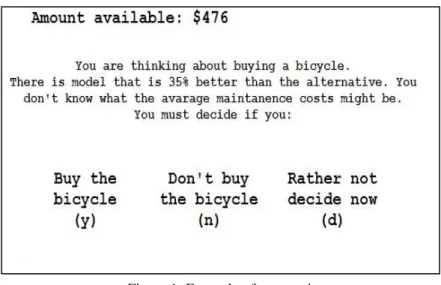
One example of a stated probability, low positive consequence scenario is: "You are thinking about buying a bicycle. There is a model that is 35% better than the alternative. You don't know what the average maintenance costs might be. You must decide if you: buy the bicycle, don't buy the bicycle or rather not decide now.", as shown in Figure 1. Scenarios differ in the presence or not of the stated probability, consequences and valences of consequences. That means that the example above might be presented in another form, representing an unstated probability, high negative consequence scenario, like: "... There is a model that is much worse than the alternative ". Phrasings of probabilities and consequences were randomized. That means that the object of the scenario would be the same (bicycle, student loan, car fixing, etc.), but the probabilities (stated or not), and consequences (high or low and positive or negative) were randomized across participants for any given object. EEG data was recorded through Acknowledge 4.4 software using an ABM B-Alert X10, composed of 9 channels (F3, F4, C3, C4, P3, P4, Fz, Cz, and Poz) and a double mastoid reference setting. Data acquisition occurred at a 256 Hz sampling rate. Behavioral data and stimulus presentation was made via PST E-Prime Professional 2.0. EEG data was analyzed using ERPLab (Lopez-Calderon & Luck, 2014). Data went through moving window artifact detection and filtered for both low and high pass (0.1 and 30, respectively). ERP epoch was set from -2000 ms before the decision was made and 200 ms after the decision was made. The use of this epoch is justified given that the information acquisition process is over before the decision is actually made, so in order to analyze event related potentials of stopping rules it is necessary to observe what happens before the decision. Behavioral data was analyzed using RStudio.
Figure 1: Example of a scenario.
Results
In order to determine the use of stopping rules and strategies for information acquisition we focus our analyses on two measures: information quantity (QTY) and balance (BAL). Information quantity is the mean amount of information pieces that each individual bought during each scenario. The balance is, just as Fifić and Buckmann (2013) proposed, one of the stopping rules that uses Bayesian calculation of the valences for each information bought. That is, if an information is positive, then the value considered is +1, if an information is negative, then the value considered is -1. At the end of a given scenario, for example, if the pieces of information acquired were 3 positives and 2 negatives (independent of order of appearance), the balance will be +1. The conditions compared to the two measures were: decision (positive, negative or procrastination), probability (stated or unstated), consequences (high or low) and valence of consequences (positive or negative).
Information acquisition
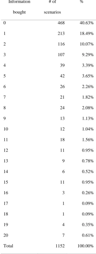
Table 1 shows the distribution of the total quantity of information bought. Given that there were 24 scenarios for each participant and 47 participants in total, the scenarios analyzed sum up to 1,152. Of the total of possible scenarios, 40.63% were decided without any kind of information acquisition, thus without the use of stopping rules. This behavior might emerge given the objects of the scenarios at hand. In order to better control the conditions, the objects of decision (car, bicycle, motorcycle purchase, student financial aid, home and car repair, investments) were less complicated. That might have made the decisions easier based on each individual set of preferences. However, there is no data to back this hypothesis. Next, there is 44.88% of the scenarios that were decided using 1 through 5 information pieces. As was previously mentioned, the order of
appearance of the information pieces was pseudorandomly presented in order to test if participants would actually follow the fixed sample or runs stopping rules proposed by Fifić and Buckmann (2013). The 14.50% of cases left used 6 through 20 information pieces.
Decision
Regarding the decisions available for the participants, the mean QTY gathered when a decision was positive is 4.11, when a decision was negative the mean QTY was also 4.11 and when participants decided to procrastinate the mean QTY was 5.04. That shows that, despite the fact that participants had up to 20 information pieces available they sought only a small amount. This behavior might suggest that the number of information acquired does not have to be a large one. Given the individual set o preferences, little amount of information is needed in order to confirm a given prior belief about a purchase or investment. On the other hand, when the BAL is considered, a positive decision was made with a mean BAL of +1.13, negative decisions were -0.73 and procrastination decisions were -0.05. That means that the information acquisition stopping point behavior is more influenced by the so called balance of the valences, regardless of the quantity of information acquired. Adding to the fact discussed above, a small amount of information needs to be purchased and when the balance hits a certain threshold, participants tend to stop information acquisition and decide. Again, that might be the case for generic and popular products/services used in this study. New products or brands might possibly show different results.
A one-way ANOVA was conducted to test for differences between each decision. The test revealed that there is a difference between the decisions both for QTY and BAL, F(2,1146)=189.9, p<0.001 and F(2,1149)=6.35, p<0.01, respectively. Post-hoc analysis using Tukey HSD test revealed significant differences between all interactions: positive-negative (p=0.001), negative-procrastination (p<0.001) and positive-procrastination (p<0.001) for BAL and only negative-procrastination (p<0.05) and positive-negative (p<0.05) for QTY.
Table 1: Quantity of information bought per scenario. Information bought # of scenarios % 0 468 40.63% 1 213 18.49% 2 116 10.07% 3 107 9.29% 4 39 3.39% 5 42 3.65% 6 26 2.26% 7 21 1.82% 8 24 2.08% 9 13 1.13% 10 12 1.04% 11 18 1.56% 12 11 0.95% 13 9 0.78% 14 6 0.52% 15 11 0.95% 16 3 0.26% 17 1 0.09% 18 1 0.09% 19 4 0.35% 20 7 0.61% Total 1152 100.00%
Probability
Analyzing only if the scenario presented stated or unstated probabilities, the only significant difference was observed in the BAL measure, F(1,1150)=4.75, p<0.05. The mean BAL for when the probability was stated was 0.031. For when the probability is not stated the mean BAL was 0.262. As for the QTY measure the mean value for the risk scenario was 4.263 and 4.100 for the uncertainty scenario.
Consequences
Although the mean values for QTY and BAL are similar to those observed in the probability analysis, no significant difference was observed in either measures. Mean values for QTY when the consequence of the scenario was high is 4.355 and 4.025 when the consequence of the scenario was low. As for BAL measure the mean values were 0.198 for high consequences and 0.095 for low consequences.
Valences of consequences
The valences of the consequences mean that a scenario can have either a positive or a negative consequence. This condition, when isolated, is the only one that has a significant difference both for the QTY and BAL measures and also presents significance when the interaction between the decision and the valence is tested in the QTY measure. The mean value for QTY when a scenario has positive consequences is 4.177 and 4.183 for a scenario with negative consequences (F(1,1146)=4.472, p<0.05). The mean value for BAL when a scenario has positive consequences is 0.063 and 0.231 for a scenario with negative consequences (F(1,1146)=42.768, p<0.001). The interaction between decision and the valence of the consequences regarding the QTY measure presented F(2,1146)=8.879, p<0.001. A post hoc Tukey HSD test revealed that the significant differences are between a positive decision in a negative consequence scenario (M=4.21) and a negative decision in a negative scenario (M=4.00) with p<0.001; a negative decision in a positive scenario (M=4.21) and a negative decision in a negative scenario (M=4.00) with p<0.001; and a positive decision in a positive scenario (M=4.04) and a negative decision in a negative scenario (M=4.00) with p=0.006.
Combining the conditions
Up until now the analysis was focused on each isolated condition. The conditions were not presented isolated for the participants. Combining the conditions yielded 8 possible scenarios, as it was previously explained, they were randomly presented three times each for the participants. If all three conditions are analyzed there is a significant difference for the
BAL measure (F(7,1128)=8.090, p<0.001). A post hoc Tukey HSD test revealed significant differences between several of the possible combinations. Of particular interest, taking into consideration the results already presented, are two. The first one is between scenarios with unstated probability, low positive consequence (M=0.118) and scenarios with unstated probability, low negative consequence (M=0.326), with p<0.001. The second one is between scenarios with stated probability, high positive consequences (M=0.007) and scenarios with stated probability, high negative consequences (M=0.181) with p<0.001.
EEG
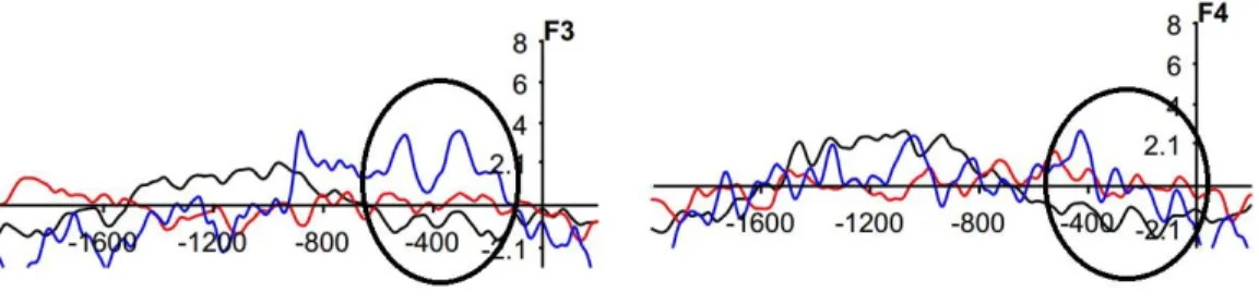
EEG analysis focused on the types of decisions and both of the combined conditions highlighted previously. Even though the epoch of the EEG analysis starts at 2000 ms before a decision is made, this part will only focus on a time frame 500 ms before the decision, given that the main effects were found at that point. The decisions show difference between positive, negative and procrastination on F3 and F4, especially a negativity for positive and procrastination decisions on F4. There is no significant difference between the electrodes or the decisions. Figure 2 shows the ERPs.
Figure 2: ERPs for decision. Left part shows ERPs for F3 electrode and right part shows ERPs for F4. Black line is positive decision, red line is negative decision and blue line is procrastination decision.
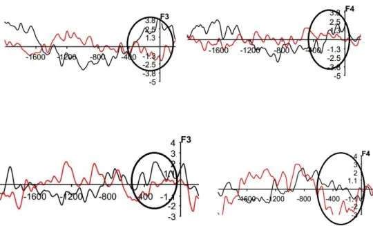
The two combined conditions also showed differences between F3 and F4. For the comparison between the unstated probabilities, low negative consequences and unstated probabilities, low positive consequences there is a negativity on F3 around 300 ms before the decision is made for the latter condition. A repeated measure ANOVA showed that there is significant interaction between the conditions and the electrodes (F(1,45)=4.096, p<0.05).
For the comparison between stated probabilities, high negative consequences and stated probabilities, high positive consequences, the difference is on the opposed electrode. There is a negativity on F4 around 400 ms before the decision is made for the latter condition. Figure 3 shows all ERPs.
Figure 3: ERPs for combined condition. Top part shows ERPs for unstated probabilities. Black line is low negative consequences and red line is low positive consequences. Bottom part shows ERPs for stated probabilities. Black line is high
negative consequences and red line is high positive consequences.
Discussion
Behavioral data suggests that the balance of acquired information (BAL) is a preferred stopping rule. Even though there was also a significant difference for the quantity of information bought and the decisions, consciously or not participants behaved according to Bayesian calculation in order to determine the end of the information acquisition process. This holds up even if the conditions are considered (combined or isolated). This means that the participants will take into account the valences of the information pieces acquired and when they reach a particular threshold (depending on the scenario characteristics or the product/service), the decision is made. That becomes clearer when the threshold is approximately +1 for a positive decision, approximately -1 for a negative decision and approximately zero for a procrastination decision. The procrastination decisions show that even though there are more pieces of information acquired, participants often would feel more uncertain and would rather skip the decision. This means that that particular scenario and the set of information acquired would not diminish the residual uncertainty acknowledged by the participant, thus making it harder to assess which decision is better given the probabilities and consequences. Another hypothesis is that the amount of information or the order of presentation made the decision ambiguous and therefore guided the participants to a procrastination behavior. This effect
resembles the 6 versus 24 jam jars example (Ariely, 2008). When given more options, individuals tend to step away from the offer, maybe because of the anxiety produced by the excess of information (Schwartz, 2004)
The analysis of the conditions suggests that participants´ behavior patterns align with prospect theory (Tversky & Kahneman, 1992). The data from this experiment suggest that uncertain scenarios are more susceptible to the quantity of information (risk seeking), higher consequences often demand more information (source dependence), and that negative consequences do have an impact on the information acquisition (loss aversion).
Scenarios where the probability was not stated (uncertain scenarios) needed less QTY and a higher BAL in order to reach a decision than a scenario where the probability is stated (risk scenarios). Higher consequences demanded more QTY and BAL than a low consequence one. If the valences of the consequences are taken into consideration, data suggests that a loss is clearly more impacting. Participants need more information in order to decide on a negative scenario. They also stop information acquisition with higher BAL for a negative scenario than for a positive scenario.
When conditions were combined, especially the two highlighted previously, the link to prospect theory is also present. If a scenario is presented with stated probabilities and high negative consequences, there is a demand for more BAL and less QTY, especially for positive and negative decisions, than with scenarios presented with stated probabilities, high positive consequences. This means that each information piece had a bigger weight at the moment when the participant would stop acquiring information. Negative consequences, meaning loss, directly affected the information acquisition process.
Taking into account scenarios with unstated probabilities, low negative consequences and scenarios with unstated probabilities, low positive consequences, there was less need for both BAL and QTY for the low positive consequences scenarios.
EEG data shows significant differences between conditions and decisions, especially in frontal electrodes. In unstated probabilities scenarios, low negative consequences present significant differences from low positive consequences. In stated probabilities scenarios, high positive consequences differed significantly from high negative consequences at F3 electrode site. This suggests that in scenarios where the uncertainty is more present, low negative consequences tend to have larger amplitudes, possibly indicating conflict between the decision and the information gathered. Similarly, in risky scenarios, high positive consequences tended to be the condition that could generate the conflict, this time with an effect at the F4 electrode site. As per the decisions, a procrastination decision was accompanied by larger amplitudes in F3 electrode than both decisions of acceptance and rejection. Although the differences present statistical significance and might be interpretable in further analyses, currently there is no inequivocal evidence, both in the data collected and in the revised literature, that can explain a lateralization effect or possible components or related components to this pre-stimulus event.
Conclusion
We developed an experiment aiming to observe different strategies, or stopping rules, that individuals might use in order to cease information acquisition and make a decision in a given scenario. Departing from the stopping rules proposed by Fifić and Buckmann (2013), the data suggests that individuals do not actually follow a particular stopping rule, rather they tend to use, consciously or not, Bayesian calculations in order consider all the information that was bought in a scenario, when considering the decisions participants made. We manipulated scenarios in order to show or not show probabilities, high or low consequences and positive or negative consequences. Those manipulations showed that the information acquisition behavior resembled prospect theory in that different levels of risk or uncertainty combined with high/low and positive/negative consequences will directly affect the quantity of information bought and the weight that the information will have in order for a participant to feel satisfied and proceed to a decision.
Future studies should try to assess the effects of different products/services and how the information acquisition process is affected. The use of known products/services versus unknown products/services might produce differences in the information acquisition process. Moreover, the use of more psychophysiological measures might shed light on some of the behaviors. Electrocardiogram and Galvanic Skin Response can further help the analysis of the decisions given the scenarios presented. Different manipulations that might further the understanding of stopping rules are time and money. Scenarios with and without time limitation and experiments with a real monetary payoff can bring the experiment closer to real life decisions.
Acknowledgments
This work was partially supported by CAPES/Brazil. We would like to thank Alicia Carmichael, Syed Tahsin, David Zhang, Lisa Jin, Donna Walter, Karen Nielsen, Jeannette Jackson and Debra Bourque for the help with this study.
References
Ariely, D. (2008). Previsivelmente irracional: As forces ocultas que formam as nossas decisões. Rio de Janeiro: Elsevier. Bland, A. R., & Schaefer, A. (2011). Electrophysiological correlates of decision making under varying levels of uncertainty.
Brain Research, 1417, 55-66. doi:10.1016/j.brainres.2011.08.031.
Courtney, H., Kirkland, J., & Viguerie, P. (1997). Strategy under uncertainty. Harvard Business Review, (December), 81–90. Di Caprio, D., Santos-Arteaga, F. J., & Tavana, M. (2014). Information acquisition processes and their continuity:
Fifić, M., & Buckmann, M. (2013). Stopping Rule Selection (SRS) Theory Applied to Deferred Decision Making. In Proceedings of the 35th Annual Meeting of the Cognitive Science Society (pp. 2273–2278). Retrieved from http://mindmodeling.org/cogsci2013/papers/0415/paper0415.pdf
Frey, R., Hertwig, R., & Rieskamp, J. (2014). Fear shapes information acquisition in decisions from experience. Cognition, 132(1), 90–99. doi:10.1016/j.cognition.2014.03.009
Gigerenzer, G. (2000). Adaptive thinking: Rationality in the real world. New York: Oxford University Press.
Kóbor, A., Takács, A., Janacsek, K., Németh, D., Honbolygó, F., & Csépe, V. (2015). Different strategies underlying uncertain decision making: Higher executive performance is associated with enhanced feedback-related negativity. Psychophysiology, 52, 367-377. DOI: 10.1111/psyp.12331.
Lopez-Calderon, J., & Luck, S. J. (2014). ERPLAB: An open-source toolbox for the analysis of event-related potentials. Frontiers in Human Neuroscience, 8, 1-14. doi: 10.3389/fnhum.2014.00213.
Martín, R. S., Appelbaum, L. G., Pearson, J. M. Huettel, S. A., & Woldorff, M.G. (2013). Rapid brain responses independently predict gain maximization and loss minimization during economic decision making. The Journal of Neuroscience, 33(16), 7011-7019. DOI:10.1523/JNEUROSCI.4242-12.2013.
Pretz, J. E., Naples, A. J., & Sternberg, R. J. (2003). Recognizing , defining and representing problems. In The Psychology of Problem Solving. Cambridge University Press.
Schwartz, B. (2004). The paradox of choice: Why more is less. New York: Harper Perennial.
Söllner, A., Bröder, A., Glöckner, A., & Betsch, T. (2014). Single-process versus multiple-strategy models of decision making: Evidence from an information intrusion paradigm. Acta Psychologica, 146, 84–96. doi:10.1016/j.actpsy.2013.12.007
Stern, E. R., Gonzalez, R., Welsh, R. C., & Taylor, S. F. (2010). Updating beliefs for a decision: neural correlates of uncertainty and underconfidence. The Journal of Neuroscience, 30(23), 8032–41. doi:10.1523/JNEUROSCI.4729-09.20104
Taghavifard, M. T., Damghani, K. K., & Moghaddam, R. T. (2009). Decision Making Under Uncertain and Risky Situations. In Enterprise Risk Management Symposium Monograph Society of Actuaries. Chicago, IL.
Tversky, A., & Kahneman, D. (1992). Advances in prospect theory: Cumulative representation of uncertainty. Journal of Risk and Uncertainty, 5(4), 297–323.
Yang, J., & Zhang, Q. (2011). Electrophysiological correlates of decision-making in high-risk versus low-risk conditions of a gambling game. Psychophysiology, 48, 1456-1461. DOI: 10.1111/j.1469-8986.2011.01202.x.
Zhang, D., Gu, R., Wu, T., Broster, L. S., Luo, Y., Jiang, Y., & Luo, Y. (2013). An electrophysiological index of changes in
risk decision-making strategies. Neuropsychologia, 51, 1397-1407.