LAGRANGIAN MODELING OF DROPLET
EVAPORATION
UNIVERSIDADE FEDERAL DE UBERLˆ
ANDIA
FACULDADE DE ENGENHARIA MECˆ
ANICA
LAGRANGIAN MODELING OF DROPLET EVAPORATION
Disserta¸c˜ao apresentada ao Programa de P´os-gradua¸c˜ao em Engenharia Mecˆanica da Universidade Federal de Uberlˆandia, como parte dos requisitos para a obten¸c˜ao do t´ıtulo de MESTRE EM ENGENHARIA MECˆANICA.
´
Area de concentra¸c˜ao: Transferˆencia de Calor e Mecˆanica dos Fluidos.
Orientador: Prof. Dr. Aristeu da Silveira Neto Coorientador: Prof. Dr. Jo˜ao Marcelo Vedovoto
Dados Internacionais de Catalogação na Publicação (CIP) Sistema de Bibliotecas da UFU, MG, Brasil.
P654L 2018
Pinheiro, Abgail Paula, 1992-
Lagrangian modeling of droplet evaporation [recurso eletrônico] / Abgail Paula Pinheiro. - 2018.
Orientador: Aristeu da Silveira Neto. Coorientador: João Marcelo Vedovoto.
Dissertação (mestrado) - Universidade Federal de Uberlândia, Programa de Pós-Graduação em Engenharia Mecânica.
Modo de acesso: Internet.
Disponível em: http://dx.doi.org/10.14393/ufu.di.2018.1180 Inclui bibliografia.
Inclui ilustrações.
1. Engenharia mecânica. 2. Evaporação - Modelos matemáticos. I. Silveira Neto, Aristeu da, 1955- (Orient.). II. Vedovoto, João Marcelo, 1981- (Coorient.). III. Universidade Federal de Uberlândia. Programa de Pós-Graduação em Engenharia Mecânica. IV. Título.
2222!"#$%&$!$'%!"(( )$!$(*'$+(+$#,$)%(%!"'1505)"$(- 020
.
/012345167638936347:8638/;34:<0617.
=>>?@ABCDE>.@>.F?>[email protected]?C@MCDE>.AH.NBGABOC?PC.QARSBPRC
TUV.W>E>[email protected][.B\.]^]^[._Z>R>.^Q[.`CZC.]^].K._CP??>.`CBaC.QbBPRC[.cdA?ZSB@PCKQL[.=NF.efghhKih]. jAZAk>BAl.megn.e]eiKg]f].K.oooVp>JG?C@VHARCBPRCVMkMVd?.K.JARp>JHARqHARCBPRCVMkMVd?.
..
r34st
u
vwxyvz{|}~uu uuuuuuuuuuuuuuuuuuuuuuuuuuuuuuuuuuuuuuuuuuuuuuuuuuuuvxwvz{
v{{yyvzuu uuu¡u u¢ uu w£y¤v{{¥¦§x£¦vz{¨¡©u u¢ uuu u
¥ª¦«¬vxv{{y¬y¤v£v{y£vz{®¯°±u²³|¨´
xw{v{£¦¦vz{µ¶·¸¹·º¸»·º¼½¾¿ÀÁ»º¸¼¾Â¼Ã¹¾ÄÁÀżÆǷľ¹·Å»¾ºÈ
£yvzuÉu¨Éu|Êu u²Ëu®Êuuuuuuuuuuuuuuuuuuuu«£yvz{Éu¨ÉuÌÍuu° ËÊ u
|u¨ÊÎÍuuv¥Ïvv{u©uÍuÐÑ}ÒuÓ uu| ÊÔu u±}ÊÔu u¡u u¢ uÕuÖu×Òu©Ð ²ÊuØÒuu©uuu u~Êu uÙÒuÚuuÙÛuu Òu©uuu~ÊuÖuÜ© Û
uuuuuuuuuuuuuuuuuuuuuuuuuuuuuuuuuuuuuuuuuuuu
Éu¨Éu|Êu u²Ëu®ÊuÝÊ ÞuÕuߢßu Éu¨ÉuÌÍuu° ËÊuÝÊ ÞuÕuߢßu
Éu¨Éu¢uÌàu u²ÓuÕuߢßu
Éu¨ÉuÌÍu±Óu¢~u u|ÓË uÕuá|
¨Éu³ u²ÊâuÕuÊ}u
. .
cdA?ZSB@PC[.^[email protected]>Ja>.@A.]h^f
ã>RMHABa>.CJJPBC@>.AZAa?>BPRCHABaA.p>?.7äåæçèé8êë85åìíèåäë80èçî[.ïäîðèææîäñëò8êî8sëóåæçôäåî85éõèäåîä[.AH.^höhfö]h^f[.÷J.^hleø[ R>Bk>?HA.O>?ù?P>.>úRPCZ.@A._?CJûZPC[.R>H.kMB@CHABa>.B>.C?aV.ø\[.ü.^\[.@>.ãAR?Aa>.B\.fVýei[[email protected].@A.>MaMd?>.@A.]h^ýV
ã>RMHABa>.CJJPBC@>.AZAa?>BPRCHABaA.p>?.äåþëäêî8æèäðëçÿ[./æé0äåî831çèä2î[.AH.^höhfö]h^f[.÷J.^hlei[.R>Bk>?HA.O>?ù?P>.>úRPCZ.@A _?CJûZPC[.R>H.kMB@CHABa>.B>.C?aV.ø\[.ü.^\[.@>.ãAR?Aa>.B\.fVýei[[email protected].@A.>MaMd?>.@A.]h^ýV
ã>RMHABa>.CJJPBC@>.AZAa?>BPRCHABaA.p>?.9äë2þåæþî83îæô8êè85îé4ë[.ïäîðèææîäñëò8êî8sëóåæçôäåî85éõèäåîä[.AH.^höhfö]h^f[.÷J.^hlei[ R>Bk>?HA.O>?ù?P>.>úRPCZ.@A._?CJûZPC[.R>H.kMB@CHABa>.B>.C?aV.ø\[.ü.^\[.@>.ãAR?Aa>.B\.fVýei[[email protected].@A.>MaMd?>.@A.]h^ýV
ã>RMHABa>.CJJPBC@>.AZAa?>BPRCHABaA.p>?.3î5î8sëäþèìî82èêîíîçî[.ïäîðèææîäñëò8êî8sëóåæçôäåî85éõèäåîä[.AH.^höhfö]h^f[.÷J.^hlg][ R>Bk>?HA.O>?ù?P>.>úRPCZ.@A._?CJûZPC[.R>H.kMB@CHABa>.B>.C?aV.ø\[.ü.^\[.@>.ãAR?Aa>.B\.fVýei[[email protected].@A.>MaMd?>.@A.]h^ýV
ã>RMHABa>.CJJPBC@>.AZAa?>BPRCHABaA.p>?.3î5î8:éå489åìóéèåäëæ8êè874èíèêî[./æé0äåî831çèä2î[.AH.^höhfö]h^f[.÷J.^hlgø[.R>Bk>?HA O>?ù?P>.>úRPCZ.@A._?CJûZPC[.R>H.kMB@CHABa>.B>.C?aV.ø\[.ü.^\[.@>.ãAR?Aa>.B\.fVýei[[email protected].@A.>MaMd?>.@A.]h^ýV
T.CMaAB6RP@C@A.@AJaA.@>RMHABa>.p>@A.JA?.R>[email protected]>.JPaA.O7pJlööoooVJAPVMkMVd?öJAPöR>Ba?>ZC@>?8A9aA?B>VpOp
CRC>@>RMHABa>8R>BkA?P?P@8>?GC>8CRAJJ>8A9aA?B>h[.PBk>?HCB@>.>.RI@PG>.UA?PúRC@>?..A.>.RI@PG>.==.33V
u
one else can make for us, which no one can spare us.”
I would like to express my sincerest gratitute to Prof. Dr. Jo˜ao Marcelo Vedovoto and Prof. Dr.
Aristeu da Silveira Neto for their constant support during these two years. Under their guidance,
with kindness and examples, they both taught me to be a better researcher. Prof. Jo˜ao Marcelo,
thank you for the inumerous encouragement words during tough moments and for the inspiring
discussions about droplet evaporation. Prof. Aristeu, thank you for the wise and phylosophical
talks about turbulence and life itself. I could not be happier with the opportunity you have given
me.
I would like to acknowledge the financial and technical support from Petr´oleo Brasileiro S.A.
(Petrobras), National Counsel of Technological and Scientific Development (CNPq), Minas Gerais
State Agency for Research and Development (FAPEMIG) and Coordination for the Improvement
of Higher Education Personnel (CAPES).
I am grateful to all friends and colleagues from MFLab for the many moments of fun and
learning. I specially thank H´elio, Bernardo, Alessandra, Marcelo, Lucas, Alex, Ricardo, Gabriel,
J´essica, Millena and Pedro for the jokes, hugs and helps. I would also like to thank Luismar, Ana
Luisa and Bruno for the technical support.
My beautiful family, Francisco, Joseilda, Andr´e, Ablail, Ana Luiza, Arg´elia e Jo˜ao Vitor,
thank you for always being by my side, no matter the distance, giving me all the support and
love I need to continue. You are my best!
My dearest Danilo, I am truthfully thankful for your everyday patience and love. Thank
you for always making me laugh.
Let´ıcia, Simone, Felipe, Marcela, Carol, Teresa Cristina, and Karina, my beloved friends,
PINHEIRO, A. P.,Lagrangian modeling of droplet evaporation. 2018. 101 p. Master
Dissertation, Federal University of Uberlˆandia, Uberlˆandia.
ABSTRACT
Evaporation of liquid droplets in high temperature gas environment is of great importance in
many engineering applications. Accurate droplet evaporation predictions are crucial in modeling
spray combustion, since it is considered a rate limiting process. For this reason, the present
dissertation aims are, first, to implement and validate Lagrangian droplet evaporation models that
are usually used in spray calculations, including equilibrium and non-equilibrium formulations, and,
second, to use these models to pursue a deeper insight on the physical phenomena that may be
involved in droplet evaporation processes. In order to validate and assess these theoretical model
predictions, an in-house code was developed and diameter evolution results from the numerical
simulations are compared to experimental data. First, the model performance is evaluated for
water in a case of low evaporation rate and, then, it is evaluated for n-heptane in moderate
and high evaporation rates using recent experimental data acquired with a new technique. The
Abramzon-Sirignano model is the only one which does not overestimate the evaporation rate
for any ambient condition tested, when compared with experimental rate. From the results, it
is also revealed that, when a correction factor for energy transfer reduction due to evaporation
is incorporated in the classical evaporation model, the predictions from this model and the
non-equilibrium one cannot be differentiated, even if the initial droplet diameter is small. Furthermore,
the incorporation of natural and forced convection effects on the droplet evaporation rate, by using
an empirical correlation, is investigated, showing that including the Grashof number into the
Ranz-Marshall correlation actually overestimates the evaporation rate for atmospheric pressure.
Finally, the effects of ambient conditions on ethanol evaporation are investigated. Under ambient
temperatures higher than the threshold temperature, the evaporation rate is enhanced with the
increase of ambient pressure, contrary to what happens for cases when the ambient temperature
is lower than the threshold temperature.
PINHEIRO, A. P., Modelagem lagrangiana de evapora¸c˜ao de gotas. 2018. 101 f.
Disser-ta¸c˜ao de Mestrado, Universidade Federal de Uberlˆandia, Uberlˆandia.
RESUMO
A evapora¸c˜ao de gotas l´ıquidas em ambientes gasosos com alta temperatura ´e de grande
relevˆancia em muitas aplica¸c˜oes de engenharia. Previs˜oes precisas da evapora¸c˜ao de gotas s˜ao
cruciais na modelagem de sprays reativos, uma vez que este ´e considerado um processo limitante.
Portanto, os objetivos da presente disserta¸c˜ao s˜ao, primeiro, implementar e validar modelos
la-grangianos de evapora¸c˜ao de gotas que s˜ao geralmente utilizados em estudos de spray, incluindo
as formula¸c˜oes de equil´ıbrio e n˜ao equil´ıbrio, e, segundo, usar esses modelos para buscar uma
vis˜ao mais profunda dos fenˆomenos f´ısicos que podem estar envolvidos no processo de
evapo-ra¸c˜ao de gotas. Para validar e avaliar as previs˜oes destes modelos te´oricos, foi desenvolvido um
c´odigo e a evolu¸c˜ao do diˆametro da gota obtida por simula¸c˜ao num´erica ´e comparada com
da-dos experimentais. Primeiro, o desempenho da-dos modelos ´e avaliado para ´agua em um caso de
baixa taxa de evapora¸c˜ao e, em seguida, para n-heptano com taxa de evapora¸c˜ao moderada e
alta usando dados experimentais obtidos recentemente por meio de uma nova t´ecnica. O
mod-elo de Abramzon-Sirignano ´e o ´unico que n˜ao superestima a taxa de evapora¸c˜ao para quaisquer
condi¸c˜oes ambiente testadas, quando comparada com a taxa experimental. A partir dos
resulta-dos, tamb´em ´e revelado que, quando um fator de corre¸c˜ao para a redu¸c˜ao da transferˆencia de
energia devido `a evapora¸c˜ao ´e incorporado ao modelo cl´assico de evapora¸c˜ao, as previs˜oes deste
modelo e do modelo de n˜ao equil´ıbrio n˜ao podem ser diferenciadas, mesmo quando o diˆametro
inicial da gota ´e pequeno. Al´em disso, a incorpora¸c˜ao de efeitos de convec¸c˜ao natural e for¸cada
na taxa de evapora¸c˜ao, usando uma correla¸c˜ao emp´ırica, ´e investigada, mostrando que a inclus˜ao
do n´umero de Grashof na correla¸c˜ao de Ranz-Marshall na verdade superestima a taxa de
evap-ora¸c˜ao para press˜ao atmosf´erica. Finalmente, os efeitos das condi¸c˜oes ambientes na evapevap-ora¸c˜ao
de etanol s˜ao investigados. Sob temperaturas ambientes superiores `a temperatura limite, a taxa
de evapora¸c˜ao aumenta com o aumento da press˜ao ambiente, contrariamente ao que acontece
nos casos em que a temperatura ambiente ´e menor que a temperatura limite.
1.1 Evaporating droplet with relative gas-droplet motion and internal circulation
(SIRIG-NANO, 1983). . . 5
1.2 Hill’s spherical vortex sketch, in which the vortex lines are complete circles at three
different times and the kidney-shaped lines are streamlines (PANTON, 2013). . . 6
1.3 Two-phase flow DNS classification into three different approaches with examples
of methods for each approach. . . 6
1.4 Schematic illustration of ocean spray (a) formation and (b) evaporation (VERON,
2015). . . 8
1.5 Simulation of a gas turbine combustor in which the fuel droplets are shown in
green (PITSCH, 2006). . . 8
1.6 Droplet suspending techniques (CHAUVEAU et al., 2008). . . 9
1.7 Global fuel ethanol production by country in 2017 in million liters with share of
global production (RFA - Renewable Fuels Association, 2017). . . 11
2.1 Schematic representation of droplet temperature evolution during its evaporation
in absence of radiation. . . 16
2.2 Schematic representation of squared droplet diameter evolution during the
evapo-ration of a single-component droplet, showing the linear behavior after the heat-up
period. . . 17
2.3 Schematic representation of an evaporating droplet surrounded by gas with vapor
mass fraction and temperature distributions along the radial direction. . . 19
2.4 Schematic representation of thermal energy and mass transfers in the evaporation
of a single droplet. . . 20
4.1 Illustration of the time lines for a Eulerian-Lagrangian simulation with∆teul >∆tlag. 33
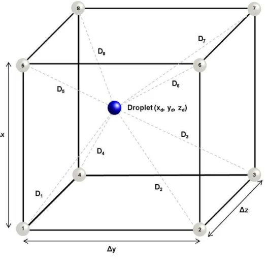
4.2 Schematic representation of the barycentric interpolation, in which the distance
between droplet and each control volume node is expressed by D. . . 36
5.1 General structure of the Lagrangian solver. . . 40
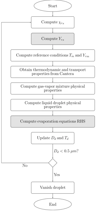
5.2 General structure of the Lagrangian evaporation function. . . 41
5.3 General structure of the Lagrangian map where cand dstand for cell and droplet, respectively. (a) Bidimensional block-structured mesh with each ID, where the black points represent the visible cells; (b) Droplets locations in the domain; (c) Multi-level hash table; and (d) Particles hash table.. . . 42
5.4 Domain partition into 8 subdomains, where each subdomain is directed to a dif-ferent processor. . . 44
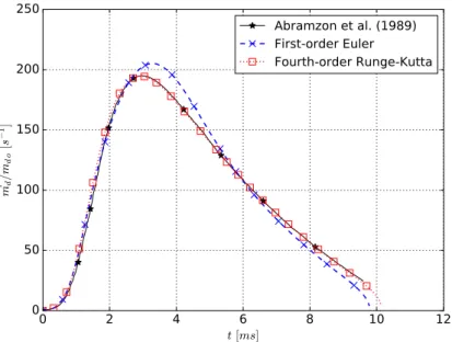
6.1 Droplet evaporation rate temporal evolution. . . 48
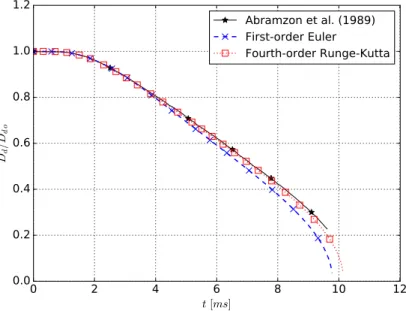
6.2 Non-dimensional droplet diameter temporal evolution. . . 49
6.3 Droplet temperature temporal evolution. . . 49
6.4 Temporal variation of normalized squared droplet diameter for water. . . 51
6.5 Temporal variation of droplet temperature for water. . . 52
6.6 Variations of normalized squared droplet diameter with the time divided by squared initial droplet diameter for n-heptane. . . 53
6.7 Variations of droplet temperature with the time divided by squared initial droplet diameter for n-heptane. . . 54
6.8 Comparison of the area evaporation rate, according to the ambient temperature, for various models and experimental measurements for n-heptane. . . 55
6.9 Temporal evolution of some evaporation parameters for equilibrium and non-equilibrium conditions with Tg = 748 K and pg = 0.1 MPa for n-heptane. . . 57
6.10 Temporal evolution of (a) the non-equilibrium contribution and (b) the ration between equilibrium and non-equilibrium vapor molar fraction for various initial droplet diameters with Tg = 748 K andpg = 0.1 MPa for n-heptane. . . 58
6.12 Variations of normalized squared droplet diameter with the time divided by squared
initial droplet diameter, with and without taking natural convection effects into
account for n-heptane. . . 61
6.13 Temporal evolutions of droplet Grashof number for the ASM* predictions
pre-sented in Fig. 6.12 for n-heptane. . . 62
6.14 Comparison of the area evaporation rate, according to the ambient temperature,
with and without taking natural convection effects into account for n-heptane. . 62
6.15 Temporal variation of normalized squared droplet diameter for n-decane. . . 63
6.16 Temporal variation of droplet temperature for n-decane. . . 64
6.17 Variations of normalized squared droplet diameter with the time divided by squared
initial droplet diameter. . . 66
6.18 Experimental, numerical and theoretical average area evaporation rates at various
ambient temperatures. . . 67
6.19 Variations of normalized squared droplet diameter with the time divided by squared
initial droplet diameter at low temperature and various ambient pressures. . . 68
6.20 Variations of normalized squared droplet diameter with the time divided by squared
initial droplet diameter at high temperature and various ambient pressures. . . . 69
6.21 Variations of droplet temperature with the time divided by squared initial droplet
diameter at low temperature and various ambient pressures. . . 70
6.22 Variations of droplet temperature with the time divided by squared initial droplet
diameter at high temperature and various ambient pressures.. . . 71
6.23 Average area evaporation rates at various ambient pressures. . . 72
6.24 Droplet final equilibrium temperature at various ambient pressures. . . 72
6.25 Schematic representation of the computational domain for the evaporation of a
single droplet. . . 73
6.26 Temporal variation of (a) normalized squared droplet diameter and (b)
tempera-ture for CEM comparing Python and MFSim predictions.. . . 73
6.27 Temporal variation of (a) normalized squared droplet diameter and (b)
6.28 Temporal variation of (a) normalized squared droplet diameter and (b)
tempera-ture for NEQ comparing Python and MFSim predictions. . . 74
6.29 Droplet evaporation for CEM simulation, in which it is colored by temperature
and its diameter reduces. . . 76
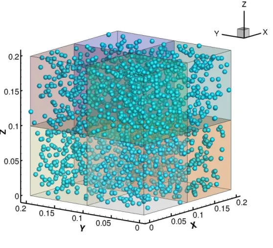
6.30 Computational domain and initial droplet diameter distribution. . . 77
6.31 Vortex flow with droplet evaporation. . . 78
6.32 Serial versus parallel computation, where the vertical lines represent the droplet
6.1 B-values for n-heptane numerical simulations . . . 53
6.2 Simulation conditions for evaporation models verification in MFSim . . . 71
Abbreviations
ASM Abramzon-Sirignano Model
ASM* Abramzon-Sirignano Model with natural convection effects
CEM Classical Evaporation Model
CEM* Classical Evaporation Model without the evaporation correction factor
CFD Computational Fluid Dynamics
CFL Courant Friedrichs Lewy
DNS Direct Numerical Simulation
ECM Effective Conductivity Model
FTM Front Tracking Method
ICM Infinite Conductivity Model
ID Identifier
LES Large Eddy Simulation
MPI Message Passing Interface
NEQ Non-Equilibrium Model
URANS Unsteady Reynolds-Averaged Navier-Stokes
VOF Volume Of Fluid
Non-dimensional numbers
BM Spalding mass transfer number
BT Spalding thermal energy transfer number
Le Lewis number
N u Nusselt number
P r Prandtl number
Sc Schmidt number
Sh Sherwood number
Red Droplet Reynolds number
Subscripts
atm Atmospheric
d Droplet
eq Equilibrium
ev Evaporation
g Ambient gas properties
h Heat-up
l Liquid properties
m Gas-vapor film properties
o Initial
s Properties at the droplet surface
v Vapor properties
Superscripts
eq Equilibrium
neq Non-equilibrium
Greek letters
αe Molecular accommodation coefficient
αw Weighting parameter for gas-vapor mixture properties evaluation
β Non-dimensional evaporation parameter
∆x Grid size in the x direction
∆y Grid size in the y direction
∆z Grid size in the z direction
δM Mass film thickness
δT Thermal film thickness
µ Dynamic viscosity
φd General droplet scalar quantity
ψ General Eulerian property
ρ Density
τd Droplet relaxation time
χv Vapor molar fraction
∆l Control volume characteristic length
∆teul Eulerian time step
∆tlag Lagrangian time step
Latin letters
˙
md Droplet evaporation rate
cp Specific heat capacity
Dd Droplet diameter
FM Correction factor for diffusional film thickness
FT Correction factor for thermal film thickness
G Correction factor for energy transfer reduction due to evaporation
K Area reduction rate
k Thermal conductivity
LK Knudsen layer thickness
Lv Specific latent heat of evaporation
md Droplet mass
p Pressure
Qd Energy effectively received at the droplet surface
QL Latent heat of evaporation
QS Sensible heat
Qg−d Total energy transferred from the gas to the droplet
Qg−v Energy carried away from droplet by diffusing vapor
Ru Universal gas constant
Tb Boiling temperature
Td Droplet temperature
Twb Wet-bulb temperature
W Molecular weight
Yv Vapor mass fraction
g Gravitational acceleration
CD Drag coefficient
Dv Vapor diffusion coefficient
ud Droplet velocity
ug Gas velocity
LIST OF FIGURES ix
LIST OF TABLES x
LIST OF SYMBOLS xi
1 INTRODUCTION 1
1.1 Background theory . . . 2
1.1.1 Evaporating droplets . . . 2
1.1.2 Computational simulations. . . 3
1.2 Motivation . . . 7
1.2.1 Applications . . . 7
1.2.2 Validation database . . . 8
1.2.3 Alternative fuels . . . 10
1.3 Objectives . . . 11
1.4 Methodology . . . 12
1.5 Dissertation outline . . . 13
2 PHYSICAL MODEL AND SIMPLIFYING ASSUMPTIONS 15 3 MATHEMATICAL MODEL 21 3.1 Displacement model . . . 21
3.2 Evaporation models . . . 23
3.2.1 Classical evaporation model . . . 24
3.2.2 Abramzon-Sirignano model . . . 28
3.2.3 Non-equilibrium model . . . 29
3.2.4 Gas-vapor mixture properties . . . 30
4 NUMERICAL MODEL 32 4.1 Time step calculation . . . 32
4.2 Time integration . . . 34
4.3 Vanishing droplets . . . 35
4.4 Interpolation method. . . 36
5 COMPUTATIONAL MODEL 38 5.1 Lagrangian solver structure . . . 39
5.2 Data structure . . . 39
5.2.1 Lagrangian map . . . 42
5.2.2 Lagrangian variables . . . 42
5.3 Search algorithm . . . 43
5.4 Parallelization . . . 44
5.5 Cantera. . . 45
5.6 Fortran/C/C++ languages linking. . . 45
6 RESULTS AND DISCUSSION 47 6.1 Abramzon-Sirignano model verification . . . 48
6.2 Evaporation models validation . . . 50
6.2.1 Water droplet with low evaporation rate . . . 50
6.2.2 N-heptane droplet with moderate to high evaporation rate . . . 51
6.3 NEQ: Langmuir-Knudsen law versus Evaporation correction factor . . . 56
6.4 Natural convection effects . . . 59
6.5 Forced convection effects . . . 63
6.6 Ambient conditions effects on ethanol evaporation . . . 64
6.6.1 Validation . . . 65
6.6.2 Effects of ambient pressure and temperature . . . 67
6.7.1 Python versus MFSim: implementation verification . . . 70
6.7.2 Vortex flow: parallelization verification . . . 72
7 CONCLUSIONS AND RECOMMENDATIONS 80
7.1 Model development . . . 80
7.2 Validation and investigations. . . 81
7.3 Main conclusions . . . 82
7.4 Recommendations . . . 83
BIBLIOGRAPHY 85
INTRODUCTION
Droplet evaporation is a complex two-phase flow phenomenon, whose modeling should take
into account the effects of transient liquid heating, gas phase convection and variable physical
properties. As a multidisciplinary issue, it can involve energy and mass transport, fluid dynamics,
and chemical kinetics. It is of primary importance in many natural physical processes and in a host
of industrial and man-related activities. This phenomenon can be found in several engineering
application fields such as, for instance, automotive and aeronautic engineering, fire suppression,
painting and medical aerosol.
Since the early work of Maxwell on this subject more than 140 years ago (MAXWELL,
2011), a relatively vast literature has become available. From these works, many valuable findings
have been reported, which helped us to increase our awareness of the key processes involved
and how devices operating conditions may impact these processes. However, this problem still
remains one of the fundamental aspects of spray investigation, to predict and improve those
systems. Thus, this area indeed requires more scientific research looking for in depth physical
insight and mathematical, numerical and computational models able to balance results accuracy
and computational efficiency.
Throughout this chapter, the purpose of the present research is elucidated and its relevance
1.1 Background theory
The background theory required to understand the role of evaporating droplets in spray
studies and the Computational Fluid Dynamics (CFD) techniques employed to simulate them are
presented in this section.
1.1.1 Evaporating droplets
Spray evaporation has been widely studied throughout the last decades, theoretically (FAETH,
1983; SIRIGNANO, 1983), experimentally (SOMMERFELD; QIU, 1998; CHEN; ST˚ARNER;
MASRI, 2006; LI; NISHIDA; HIROYASU,2011), and numerically (SADIKI et al., 2005; JONES;
LYRA; MARQUIS, 2010; DE; LAKSHMISHA; BILGER, 2011; AZAMI; SAVILL, 2016;
ABDEL-SAMIE; TH´EVENIN, 2017). However, considering the complexity of such theme, an isolated
droplet evaporating in gas medium, which represents an ideal model of the physical phenomena
involved in the diluted regions of a spray, seems to be a first step towards better understanding
the evaporation dynamics. Even though the case of a single isolated droplet might seem just as
an idealization, in most technical applications where the spray can be considered dilute, this
as-sumption is actually reasonable (JENNY; ROEKAERTS; BEISHUIZEN, 2012). Dense dispersed
two-phase flows are not in the scope of the present work, since the isolated droplet assumption
is no longer valid.
Evaporating sprays can be classified as dispersed two-phase flow, containing a liquid as the
dispersed phase in the form of droplets and a gas as the continuous carrier phase. The volume
fraction of the dispersed phase, αd, is the volume occupied by the droplets in a unit volume of
the continuous phase, V. Hence, this property is given by:
αd=
PNi
1 Vdi
V , (1.1)
where Ni is the number of all droplets in the control volume, having each droplet volume as
Vdi=πDdi3/6. According to Sommerfeld(2017), a dispersed two-phase flow may be considered
in a dilute regime when the volume fraction is lower than5x10−4
or the mean inter-droplet spacing
As defined byAshgriz(2011), evaporation is a process of phase transition in which molecules
in a liquid overcome the intermolecular attraction forces and escape into the surrounding gaseous
medium. When energy is supplied to a liquid, its temperature and, hence, the kinetic energy of
the liquid molecules, are augmented, resulting in an increase of the evaporation rate. When the
ambient pressure diminishes, the chances of the liquid molecules near the surface to overcome
their intermolecular attraction potential increases, also resulting in an increase of the evaporation
rate.
Therefore, droplet evaporation process basically consists in two main stages. First, vapor
molecules detach from the droplet surface into the surrounding gas in the immediate vicinity of
the droplet. Then, these vapor molecules diffuse away from the droplet surface into the ambient
gas due to the concentration gradient.
Sazhin (2006) states that, as the mathematical modeling of the first stage is extremely
complex, in most practical applications the first stage is neglected and the assumption that vapor
in the vicinity of the droplet surface is always saturated is adopted. Thus, the evaporation rate
is actually equals to the vapor diffusion rate. The evaporation models that follow this vapor
saturation assumption are called dynamic models.
Sazhin(2006) also presents evaporation models that consider the vapor molecules
detach-ment, such as the kinetic models, which are based on Boltzmann transport equation, and the
molecular dynamics models, that model the dynamics of each individual molecule.
Even though the description of the evaporation process is based on a molecular viewpoint,
the present work is based on the continuum hypothesis by using the fundamental balance equations
for mass, energy and linear momentum for liquid and gas phases, together with the appropriate
interfacial conditions, i.e., droplet surface boundary conditions, initial conditions, and relevant
thermodynamic relations, as presented in Chapter 3. As a consequence, only dynamical models
are studied and implemented in the present research, since for practical applications computational
cost and accuracy should be balanced. The simplifying assumptions made for the derivation of
1.1.2 Computational simulations
In the past decades, CFD has become a very powerful tool, both in academic research
and industrial applications, and it has been increasingly employed to analyze processes and to
support engineering decisions. However, application of CFD in two-phase flow simulations is pretty
young, probably having started only around 40 years ago, due to the complexity of the physical
phenomena involved in them (SOMMERFELD,2017). Evaporating sprays, which are an example
of two-phase flows, may involve several phenomena, such as: jet breakup and atomization; droplet
collision and coalescence by droplet-wall and droplet-droplet interactions; mass, energy and linear
momentum transfers by droplet-gas interaction (SCHWARZKOPFet al., 2011).
Even though there exist various challenges to model those problems, computational
simula-tions are often preferred over material experiments because of the following reasons: (i) they can
overcome some of the difficulties related to control external perturbations in order to maintain
the conditions assumed by theoretical models throughout the whole test; (ii) since parameter
imposition is easier in computational simulations, they can be used to study a much wider range
of conditions, which allows to study the influence of individual operating parameters on
indus-trial device performances; (iii) the submillimeter scales associated with the evaporating-spray
problem have made detailed experimental measurements very difficult in terms of catching the
fluid-dynamical characteristics of this flow; and (iv) computational simulations may be carried
out faster due to a shorter lead-time, and with less expenses, depending on the studied problem
(LIU,1999).
A Direct Numerical Simulation (DNS) of single-phase flows may be defined as solving the
Navier-Stokes equations, coupled with the continuity equation, for all the turbulent scales in the
flow field. For two-phase flows, on the other hand, it implies on the resolution of the gas phase
around each droplet and the whole field of droplets. In this context, three distinct approaches
can be adopted in order to perform a two-phase flow DNS: Eulerian (E-E),
Eulerian-Lagrangian (E-L) with resolved droplet and Eulerian-Eulerian-Lagrangian with point droplet approximation
(JENNY; ROEKAERTS; BEISHUIZEN, 2012).
The Eulerian-Eulerian approach is based on interface capturing methods to describe the two
may be the volume fraction, which represents the amount of each phase in each computational
cell of the domain. The interface position is inferred by the value of the marker function. The
most used interface capturing methods are the volume of fluid (VOF) and the level set methods.
The VOF method, for instance, treats the multiphase flow using the “one-fluid” approach, with
fully Eulerian formulation, only using a marker function to represent the existence of multiple
phases. Some examples of DNS studies using the Eulerian-Eulerian approach are Schlottke and
Weigand(2008), Lee, Riaz and Aute (2017) and Deising, Bothe and Marschall(2018).
The Eulerian-Lagrangian approach with resolved droplet applies interface tracking methods,
such as front tracking methods (FTM). These methods represent the interface between phases
with a set of Lagrangian marker points and this interface is advected in a Lagrangian fashion,
while the flow equations for both phases are solved on a Eulerian grid. The extra forces, calculated
on the marker points, are added to the right hand side of the flow equations in order to mimic the
boundary conditions at the interface. The fluid dynamic forces and gravitational forces on the
droplet are used to calculate its motion and rotation. It is crucial that no approximation of these
forces and torques be made. The boundary conditions corresponding to each and every droplet
surface should also be included. Thus, good resolution of the velocity, pressure, temperature
and concentration gradients in the droplet vicinity is required to precisely determine the coupling
terms, which express the linear momentum, thermal energy and mass transfer rates between
phases. Some examples of DNS studies using the Eulerian-Lagrangian approach with resolved
droplet are Irfan and Muradoglu (2017) and Fang et al. (2018).
The Eulerian-Lagrangian approach with point droplet approximation also applies
contin-uum equations for the gaseous phase, but droplet evaporation rate, temperature change and
acceleration are actually modeled. The point droplet approximation approach may be a good
choice when droplet sizes are below the Kolmogorov length scale, since the droplets will not
in-terfere with the resolved spectrum. Some examples of DNS studies using the Eulerian-Lagrangian
approach with point droplet approximation are Xia and Luo(2009), Wang, Luo and Fan (2014)
and Abdelsamie and Th´evenin (2017). Sirignano (2010) presents some evaporation models that
differ from each other in the treatment of the liquid phase heating, which is usually the
rate-controlling phenomenon in droplet evaporation, particularly in high-temperature gas environment.
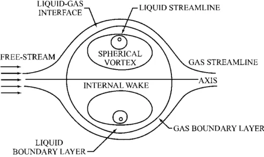
internal liquid circulation driven by surface-shear forces, as displayed in Fig. 1.1, are considered
or not.
Figure 1.1: Evaporating droplet with relative gas-droplet motion and internal circulation (SIRIGNANO, 1983).
The infinite-liquid-conductivity model (ICM), with uniform but time-varying droplet
tem-perature, assumes that the thermal conductivity of the liquid phase is infinitely large and that
there is no temperature gradient inside the droplets. The effective conductivity model (ECM)
takes into account both finite liquid thermal conductivity and the re-circulation inside droplets
via the introduction of a correction factor to the liquid thermal conductivity, that is determined
as a function of the liquid phase P´eclet dimensionless number and varies from about 1 to 2.72
(ABRAMZON; SIRIGNANO,1989). Moreover, there are vortex models for droplet heating, which
describe the re-circulation inside droplets in terms of vortex dynamics to represent the physical
situation of advective heating. The well-known Hill’s spherical vortex, which is illustrated in Fig.
1.2, is usually used as a vortex model (HILL, 1894; BATCHELOR, 2000). In Figure 1.3, a chart
summarizing all the possible approaches for computing a two-phase flow DNS, as described above,
is displayed.
Considering that, in real-world problems, evaporating droplets are typically of the order of
a few tens of micrometers to a few hundreds of micrometers in diameter, very fine computational
grids are required to properly capture the whole detailed physics of these problems. Moreover,
resolution of internal droplet gradients can imply resolution on a submicrometer scale, which can
ing problems, species and thermal energy balance equations would also have to be contemplated,
together with the continuity and Navier-Stokes equations. Consequently, DNS of two-phase flows
using the Eulerian-Eulerian approach is limited to canonical test cases in academic research to
be available as references and to gain physical insight. Meanwhile, DNS studies applying the
Eulerian-Lagrangian approach with resolved droplets accounting for a large number of droplets is
also not within current computational feasibility.
Several Lagrangian models for describing the dispersed phase evolution exist, for droplet
dynamics and evaporation itself. These models are usually coupled with Large Eddy Simulation
(LES) or Unsteady Reynolds-Averaged Navier-Stokes (URANS) methodologies for the gaseous
continuous phase by means of sources terms. The focus of the present dissertation is the
La-grangian evaporation models, more specifically infinite-liquid-conductivity models, presenting their
mathematical formulation in Chapter 3 and evaluating their predictions in Chapter 6.
1.2 Motivation
This section is dedicated to present the motivation that justifies the dissertation theme
relevance. First, the main applications in which droplet evaporation can be found are illustrated.
Second, the need of validating theoretical models with recent experimental data is explained.
Third, the concern over greenhouse-gas emissions and the search for renewable fuels as an
alter-native to the petroleum sources are addressed.
1.2.1 Applications
Liquid droplet evaporation process can be observed in both nature and technological
ap-plications. In the environment, for example, such phenomenon occurs in ocean sprays (see Fig.
1.4) and rainfalls. In industry, it is mainly noticed in energy systems, such as furnaces, chemical
reactors, gas turbines, internal combustion engines, among others (LEFEBVRE; MCDONELL,
2017). More specifically, evaporation of liquid droplets in high temperature gas environment
plays an important role in technical applications involving combustion of liquid fuels. Due to
improper handling, most of these devices are not operated under optimal conditions. Therefore,
could improve industrial processes.
Figure 1.4: Schematic illustration of ocean spray (a) formation and (b) evaporation (VERON,
2015).
(a)
(b)
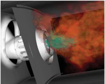
In a gas turbine combustor, as represented in Fig. 1.5, basically, the liquid fuel jet is
injected and atomizes into several droplets to generate a polydisperse spray with multiple droplets
of different sizes, which evaporate in the hot gaseous medium. Then, the vapor fuel mixes with
the oxidant and, finally, burns. In this context, accurate prediction of vapor fuel concentration is
essential to correctly model the whole spray combustion process. Some parameters, as droplet
evaporation rate and lifetime, are critical for design and operation of those devices (TURNS,
2000). As a conclusion, droplet evaporation modeling is crucial to increase efficiency and reduce
Figure 1.5: Simulation of a gas turbine combustor in which the fuel droplets are shown in
green (PITSCH, 2006).
1.2.2 Validation database
Since spray simulations results are strongly influenced by the droplet evaporation model
adopted, validation of theoretical models is indispensable. Miller, Harstad and Bellan (1998), for
instance, already reviewed most of the well-established droplet evaporation models that are usually
used in spray simulations to examine their validity. By means of an extensive model comparison
accounting for eight different models and considering five different liquids for cases of low to high
evaporation rates, they have concluded that, in general, the non-equilibrium formulation agrees
most favorably with a wide range of experimental measurements. Nevertheless, their conclusions
were based on experimental measurements whose accuracy may have been deteriorated by extra
energy sources, which are not part of the physical model considered to develop the droplet
evaporation models.
To begin with, the majority of experiments performed to study the evaporation of a single
droplet, specially the elder ones, have used the classical single fiber technique, in which the droplet
is suspended by a fiber. However, some studies (YANG; WONG, 2002; GHATA; SHAW, 2014)
have already shown that the single fiber technique actually increases the droplet evaporation rate
significantly, since there is an energy transfer from the fiber to the droplet through conduction.
For smaller droplets, the presence of positioning fibers or thermocouples influences even more the
evaporation rate, considering that those devices have a non-negligible diameter compared to the
Secondly, some experiments, as, for instance, the one presented in Nomura et al. (1996)
for a single n-heptane droplet at a wide range of ambient conditions, also have a contribution of
the radiation emitted by the internal walls of the furnace where tests were conducted (YANG;
WONG, 2001).
In order to assure experimental data reliability, recent experiments have been more mindful
to avoid those extra energy sources by using new techniques. Therefore, there is a need to better
investigate the validity of theoretical droplet evaporation models by comparing their predictions
against experimental measurements performed applying those new techniques.
Chauveau et al. (2008), for example, used the cross-fiber technique in order to avoid
conduction effects. For this new experimental approach for the characterization of evaporating
droplets, the fiber diameter is 14 µm, whereas, for the single fiber technique, traditional fiber
diameters are larger than 120µm. Chauveauet al.(2008) have concluded that the droplet
evap-oration rate increases linearly with the fiber cross-sectional area, corroborating the use of the
cross-fiber technique. The cross-fiber technique also ensures droplet spherical shape (VERWEY;
BIROUK, 2017), which is an assumption usually adopted in theoretical models, without
micro-gravity condition, as showed in Fig. 1.6. Moreover, while the experimental data using suspended
technique are limited to rather large droplets, the cross-fiber technique enables more realistic
ex-periments, considering that spray Sauter mean diameters tends to be below 100µm for practical
purposes in the combustion area (LEFEBVRE, 2010).
Figure 1.6: Droplet suspending techniques (CHAUVEAU et al., 2008).
(a) Classical single fiber (b) Cross-fiber
Finally, it is important to highlight that for validation of theoretical models choosing
ex-periments performed under conditions closer to the assumptions adopted for their derivation is
gravity, but this technique actually introduces convective effects due to the slip velocity and a
certain degree of asymmetrical evaporation, which violates the spherical symmetry assumption
usually adopted. In order to eliminate these convective and buoyancy effects, experiments have
to be performed in drop towers or parabolic flights to achieve microgravity condition, increasing
the experimental set-up complexity and cost.
1.2.3 Alternative fuels
In 2012, fossil fuels accounted for 84% of worldwide energy consumption. In 2040, even
with the increase in renewable and nuclear energy, predictions have shown that fossil fuels will still
account for 78% of energy use (IEA - International Energy Agency, 2016). As a consequence,
the majority of the work that has already studied effects of ambient pressure and temperature
on droplet evaporation focused on fossil fuel components evaporation. However, as stated by
Bergthorson and Thomson (2015), there is a huge concern over greenhouse-gas emissions and
petroleum scarcity that motivates a search for alternative fuels. In this context, ethanol is
con-sidered a clean, efficient, and affordable energy source solution.
Ethanol is considered a promising alternative fuel because it is derived from biomass via
established and new processes, as proved by the evolution from first to third-generation biofuels;
it seems to be easy merging its production and use with the existing infrastructure; and it has
ad-vantages when compared with conventional fuels. If compared with gasoline, to illustrate, ethanol
has a significantly higher octane number and latent heat of evaporation, which improves thermal
and volumetric efficiencies and may reduce emissions of pollutants, such as carbon monoxide,
ex-haust hydrocarbons and fine particulates (AGARWAL, 2007; WESTBROOK, 2013; QUIROGA;
BALESTIERI; ´AVILA,2017).
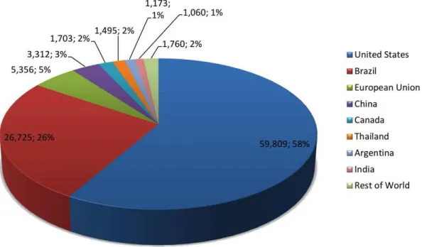
Ethanol may be considered the most widely used biofuel in the world (SARATHY et al.,
2014), concentrating its largest production in the United States, followed by Brazil. In 2017,
these two countries accounted for about 84% of the total global fuel ethanol production, which
was approximately 87 billion liters (RFA - Renewable Fuels Association, 2017), as presented in
Fig. 1.7. The use of pure ethanol as automotive fuel is mainly limited to Brazil, while blends
with gasoline are mostly used as fuels in Europe, United States, China and Canada (CORSETTI
blends (SAZHIN et al., 2010; CAMPOS-FERN´ANDEZet al., 2012; BADER; KELLER; HASSE,
2013;MAet al.,2015;QUBEISSI; SAZHIN; ELWARDANY,2017;YIet al.,2017;KUSZEWSKI,
2018) as an alternative to pure fossil fuels that would not drastically change evaporation and
combustion characteristics in the already existing engines.
Figure 1.7: Global fuel ethanol production by country in 2017 in million liters with share of
global production (RFA - Renewable Fuels Association,2017).
Many experiments have been performed to study droplet evaporation for different fuels
and under several ambient conditions (WONG; LIN, 1992; NOMURA et al., 1996; GHASSEMI;
BAEK; KHAN, 2006; CHAUVEAU et al., 2008; HASHIMOTO et al., 2015; HAN et al., 2016;
BORODULIN et al., 2017). The effects of ambient pressure on n-heptane and kerosene droplet
evaporation have been experimentally examined by Nomura et al. (1996) and Ghassemi, Baek
and Khan(2006), respectively. Both of them stated that droplet lifetime decreases monotonically
when gas temperature increases. Nonetheless, as pressure increases, evaporation rate increases at
low gas temperature and decreases at high temperature. Similarly,Harstad and Bellan(2000) and
Kitano et al. (2014) numerically studied those effects on n-heptane and n-decane droplets and
arrived to the same conclusions. Although some of these authors have studied the evaporation
dynamics under technical system typical conditions, none of them analyzed the effects of ambient
conditions on evaporation of pure ethanol droplets.
im-pacts in the ethanol evaporability is performed aiming to make feasible the development of new
technologies for ethanol-fueled internal combustion engines, resulting in more functional and
economical devices. This motivation is specially important in what concerns Brazilian interests.
1.3 Objectives
The main objectives of the present dissertation are, first, to implement and validate
La-grangian droplet evaporation models, and second, to use these models to pursue a deeper insight
on the physical phenomena that may be involved in the droplet evaporation process. Therefore,
the specific objectives are:
• To review some existing models for droplet evaporation under the Lagrangian approach
that are usually used for academic research and industrial applications;
• To develop the physical and mathematical models of the studied problem proposed taking
into account the key processes involved, such as mass, energy and momentum transfers
between phases;
• To evaluate and compare different evaporation models;
• To implement those evaporation models in the in-house code MFSim, which is under
de-velopment in the Fluid Mechanics Laboratory of the Federal University of Uberlˆandia;
• To validate evaporation model predictions by comparison with experimental measurements
reported in literature;
• To investigate ambient condition influences on droplet evaporation rate.
1.4 Methodology
The Eulerian-Lagrangian approach, has been widely employed for dilute spray simulations,
where the droplets are represented as point sources. Thus, each individual droplet is tracked
in its own frame of reference and ordinary differential equations are considered to determine
position, velocity, diameter and temperature temporal evolution of each droplet. These equations
Point droplet approximations are well justified for droplet sizes below the Kolmogorov length
scale, as in the cases studied in the present research. However, this approach can be problematic
for larger droplets, demanding an additional modeling to properly account for the interference of
the dispersed phase in the flow field.
To study any physical phenomenon, the coming steps should be considered:
• Description of the physical model that represents the problem of interest and the simplifying
assumptions;
• Derivation of the mathematical model based on the assumptions;
• Definition of the numerical schemes used to solve the equations proposed in the
mathe-matical model;
• Implementation of the computational model;
• Verification and validation of the code to assure its reliability;
• Simulations to investigate new configurations;
• Discussion of the obtained results.
The focus of the present dissertation is not only on the physical modeling of droplet
evaporation, but also on the further development of an existing CFD software, the in-house code
MFSim that is presented in Chapter 5. Therefore, a massive amount of knowledge and effort is
required to translate differential and algebraic mathematical equations into algorithms and code
lines.
1.5 Dissertation outline
The present dissertation consists of 7 chapters and 1 appendix. In Chapter 1, which was
already presented, the authors present some background information of the present work, clarify
the motivation and objectives, and draw an overall picture of the studies that are conducted,
including the methodology followed.
Problem modeling was divided into four topics: physical, mathematical, numerical and
the physical model and state the main simplifying assumptions adopted. In Chapter 3, the
math-ematical models used to represent the droplet evaporation process treated with the Lagrangian
approach are reviewed. In Chapters 4 and 5 some aspects of the numerical and computational
models are explained, such as time integration schemes, interpolation algorithm, parallel
imple-mentation and the Lagrangian solver.
In Chapter6, the authors show the results and discussions. The results comparing two time
integration schemes are presented in the first section. Droplet evaporation model validation for
water and n-heptane is presented in the second section. Once the models are verified, validated
and evaluated, non-equilibrium effects are studied in the third section. Natural convection effects
are investigated for n-heptane and forced convection effects are analyzed for n-decane in the
fourth and fifth sections, respectively. Ambient condition effects are studied for ethanol in the
sixth section and, finally, the seventh section presents some simulations performed with the
in-house code MFSim.
In Chapter 7, the authors summarize the major findings, present the conclusions and give
the recommendations for future work. The last part, Appendix A, has been dedicated to display
some implementation details of the evaporation routines added into MFSim, more specifically, the
PHYSICAL MODEL AND SIMPLIFYING ASSUMPTIONS
Knowing that the evaporation process is quite complex and depends on many factors, it
becomes necessary to adopt some hypotheses to simplify the models that represent it. As long
as the point droplet approximation is adopted, as stated in Section 1.4, the description of the
dispersed phase reduces to modeling the phenomena acting on the droplets. Considering the
restrictions imposed by computational requirements and the purposes of the present research,
some simplifying assumptions are considered when modeling droplet evaporation. The main
simplifications employed to the description of the dispersed phase are given in the next paragraphs.
Droplets are treated as spherical non-deformable liquid structures, meaning that breakup
mechanisms are not modeled. For droplets larger than the Kolmogorov scale, transient
defor-mation occurs and the evaporation behavior becomes more complex. Since for high liquid-gas
specific mass ratio the droplet equation of motion is governed mainly by drag and gravity forces,
the other forces acting on the droplet will be neglected, as presented in Section 3.1.
Droplet-droplet interactions, such as collisions and coalescence, are assumed negligible.
Energy transfer between liquid and gaseous phases is assumed to occur only through
con-vection, neglecting radiation. During the initial stage of the droplet lifetime, a transient heat-up
period, the energy received by the droplet is utilized to heat-up the liquid to its equilibrium
temperature. Once this temperature is achieved, all the energy transferred into the droplet is
droplet surface is zero, so the droplet temperature, Td, remains constant.
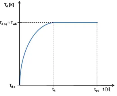
Due to the balance between heating and cooling, liquid droplets usually do not reach
the boiling point, Tb, when they are heated. Instead, in absence of radiation, the temperature
evolves towards the wet-bulb temperature, Twb, approaching it asymptotically (ABRAMZON;
SAZHIN, 2005; ABRAMZON; SAZHIN, 2006), as displayed in Fig. 2.1. Subscripts o and eq
refer to initial and equilibrium droplet temperatures, while subscripts h and ev refer to
heat-up and total evaporation times. The droplet temperature evolution is determined by a balance
between conductive heating and evaporative cooling, and the droplet equilibrium temperature
value reached depends on the ambient conditions.
Figure 2.1: Schematic representation of droplet temperature evolution during its evaporation in absence of radiation.
After the initial heat-up period, the well-known D2
law is obeyed, which means that the
square of the droplet diameter, Dd, decreases linearly with time. This behavior occurs because
energy and mass diffusion in the surrounding gaseous film are the rate-controlling processes.
Therefore, an area reduction rate, K, can be estimated as the negative slope of the variation of
the squared droplet diameter in the steady-state evaporation period, as represented in Fig2.2.
The liquid is composed of a single chemical specie, so no multicomponent aspects are
considered. For multicomponent cases, a deviation from theD2
law is expected, since the more
volatile substances evaporate faster, and mass diffusion in the liquid phase becomes important.
con-Figure 2.2: Schematic representation of squared droplet diameter evolution during the evap-oration of a single-component droplet, showing the linear behavior after the heat-up period.
ductivity model is adopted, which is also called in the literature as the rapid mixing model. The
thermal conductivity in the liquid phase is assumed infinite, which results in a homogeneous
tem-perature distribution over the droplet volume. Even though the droplet temtem-perature is considered
as uniform, it still varies with time. According toMa(2016) and Sazhin(2017), the infinite
con-ductivity model is usually used for academic research and industrial applications CFD simulations
due to its computational efficiency and easy implementation.
Droplet inner flow is not computed and the effects of temperature gradient inside droplets
are ignored. Resolving the internal droplet recirculation flow increases the computational cost
significantly because a differential equation needs to be solved for the liquid temperature.
How-ever, this does not lead to better predictions of droplet diameter or temperature for cases with
small droplet initial diameter (BEISHUIZEN,2008).
The evaporation rate of the single droplet is calculated under the assumption that the
variations of the gas temperature and vapor mass fraction caused by the droplet evaporation
are negligibly small. In other words, the isolated droplet evaporation does not affect the infinite
gaseous medium conditions. This assumption is in fact reasonable for a dispersed two-phase
flow case. However, for dense two-phase flows, it was proved that increasing the number of
droplets per unit volume reduces the evaporation rate (VOLKOV; KUZNETSOV; STRIZHAK,
For ambient pressure and temperature below the critical condition, the droplet remains in
the liquid state throughout its whole lifetime. The liquid specific mass is much larger than that of
the surrounding gas, while the thermal diffusivity in the gas phase is much larger than the
liquid-phase thermal diffusivity. The large ratio between the liquid-phases properties implies that the liquid
phase has higher thermal and mass inertia as compared to the gas phase. Therefore, the processes
that occur in the gas phase can be assumed to be quasi-steady. This assumption indicates that
the gas-phase immediately adjusts itself to the local boundary conditions and droplet size at each
instant of time.
A quasi-steady assumption is often made for the gas-phase because energy and mass
dif-fusion is usually relatively fast compared with that of the liquid. This assumption weakens as
the critical condition is approached. According to Sirignano and Law (1978), for near-critical
or supercritical evaporation occurring typically in rocket motors and diesel engines, for instance,
unsteady gas-phase analysis are required, meaning that the gas-phase time derivatives should be
retained for the evaporation model derivation. Only droplet evaporation in subcritical conditions
is evaluated in the present research; however, further discussions of models validity and droplet
evaporation behavior in near-critical and supercritical conditions can be found inSirignano(2010),
Kontogeorgis and Folas (2010), Bellan (2000) and Givler and Abraham(1996).
Spherical symmetry is also assumed, meaning that convection is absent and, hence, droplet
remains spherical during its whole lifetime. The effects of natural and forced convection are
taken into account using empirically established laws, since convective effects generate a certain
degree of asymmetrical evaporation. These effects are usually expressed introducing correlations
to Nusselt and Sherwood numbers by incorporating Reynolds and Grashof numbers into their
calculations. Different empirical correlations are available in the scientific literature (FR ¨OSSLING,
1938; RANZ; MARSHALL, 1952a; CLIFT; GRACE; WEBER, 1978; RENKSIZBULUT; YUEN,
1983;KULMALA et al., 1995), and they have been implemented either in single droplet or spray
calculations.
Thermal energy flux can be generated not only by the existence of temperature gradients,
but also by concentration gradients. Similarly, mass flux, which is provided by concentration
gradients, can also be promoted by temperature gradients. The energy flux caused by
known as Soret effect. These two effects occur simultaneously and they are secondary diffusion
processes. In the present research, Soret and Dufour effects are not considered, since their order
of magnitude is much smaller than that of Fick and Fourier laws (SAZHIN, 2006).
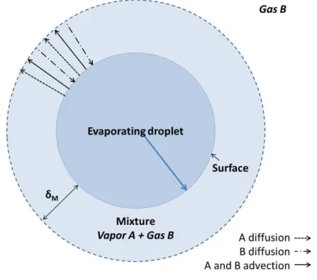
In Figure 2.3, the authors illustrate the described physical model, in which Yv represents
vapor mass fraction,Rdrepresents droplet radius, and subscriptssand g, refer to droplet surface
and far from the droplet or out of the gas-vapor film, respectively. In Figures 2.4a and 2.4b,
the authors show the mass and energy transfers involved in the evaporation of a single droplet,
where δM and δT represent the thicknesses of the mass and thermal films, respectively. These
surrounding gaseous films are always treated as a mixture of vapor and ambient gas.
From Fig. 2.4b, one can see that the energy effectively received at the droplet surface,
Qd, is equal to the sum of the latent heat of evaporation,QL, and the sensible heat, QS, and it
is also equal to the difference between the total energy transferred from the gas to the droplet,
Qg−d, and the energy transferred from gas to vapor that is carried away from droplet by diffusing
vapor in form of superheat,Qg−v.
Figure 2.4: Schematic representation of thermal energy and mass transfers in the evaporation of a single droplet.
(a) Sketch of the mass transfer in the evaporation of a single droplet, in which vapor A advective transport represents the well-known Stefan’s flow, which is explained in Section3.2.
MATHEMATICAL MODEL
Accurate droplet displacement and evaporation predictions are crucial in modeling dilute
spray evaporation, since they are considered rate limiting processes (JENNY; ROEKAERTS;
BEISHUIZEN,2012). Some parameters, as vapor concentration and droplet lifetime, are specially
important for design and operation of energy systems. With this in mind, the purpose of this
chapter is to present the mathematical formulation used to represent those processes.
3.1 Displacement model
For engineering applications involving spray evaporation, the droplet drag force and the
gravitational force, also known as body force, are predominant compared to other forces, as Basset
history, added mass, Magnus, Saffman, buoyancy and pressure gradient terms (SHIROLKAR;
COIMBRA; MCQUAY,1996). Under these conditions and considering the Lagrangian approach,
droplet motion and momentum equations are:
dxd
dt =ud, (3.1)
dud
dt =
ug−ud
τd
where xd andudare droplet position and velocity, respectively, ug is the carrier gas velocity, and
g is the gravitational acceleration. The droplet relaxation time, τd, is determined by:
τd = 4 3
ρl
ρg
Dd
CD|ug−ud|
, (3.3)
where ρl and ρg respectively refer to liquid droplet and gas phase densities. The drag coefficient,
CD, is given by semi-empirical correlations. A frequently used one is the Schiller-Naumann
correlation for solid non-evaporating spheres, which is given by (CLIFT; GRACE; WEBER,1978):
CD =
24
Red, if Red<0.1
24
Red(1 + 0.15Red)
0.687
, if 0.1< Red≤1000
0.44, if Red>1000
, (3.4)
in which the droplet Reynolds number, Red, is defined as:
Red =
ρgDd|ug −ud|
µg
, (3.5)
where µ is the dynamic viscosity.
Since the Stefan’s flow reduces the drag coefficient (ABRAMZON; SIRIGNANO, 1989),
Sazhinet al. (2005) have suggested a modification ofCD for evaporating droplet:
CDev =
CD
(1 +BM)α
M, (3.6)
where BM is the Spalding mass transfer number given by:
BM =
Yvs−Yvg
1−Yvs
, (3.7)
respectively, andαM is:
αM =
1, if BM <0.78
0.75, if BM ≥0.78
. (3.8)
3.2 Evaporation models
Introductory descriptions of evaporating droplet behavior can be found in the work of
Williams (1985), Kuo (2005) and Turns (2000), while a comprehensive and in-depth discussion
of droplet evaporation under a variety of conditions can be found in the classical textbook of
Sirignano (2010). Furthermore, useful research reviews are given by Sazhin (2006) and Sazhin
(2017) summarizing various droplet evaporation and heating models, with different levels of
complexity. In these reviews, it is also pointed out that detailed models based on single droplet
analysis have to be simplified to simulate evaporating spray using CFD methodologies aiming at
computational efficiency.
In this chapter, some standard single droplet evaporation models are presented taking
into account the two key processes involved in the evaporating phenomenon, mass and energy
transfer. These processes are described by differential equations, which express the temporal
changes of droplet size and temperature. Considering the assumptions presented in Chapter 2,
these equations are:
dmd
dt =−m˙d, (3.9)
wheremdis the droplet mass andm˙d is the droplet evaporation rate that leads directly to droplet
size reduction:
dDd
dt =−
2 ˙md
πρlDd2
and
dTd
dt = QS
mdcpl
, (3.11)
wherecplis the liquid droplet specific heat capacity and recalling thatQS is the power transferred
to promote the droplet thermal energy variation per unit of time, which is transferred as heat.
3.2.1 Classical evaporation model
The basis of the theory on droplet evaporation in gaseous medium was laid by Maxwell.
Back in 1877 (MAXWELL, 2011), he proposed the simplest evaporation model, considering
the stationary evaporation rate for a spherical droplet, motionless relative to an infinite and
uniform gaseous medium. In addition, the concentration of the vapor at the droplet surface was
assumed to be equal to its equilibrium concentration, or, in other words, the saturated vapor
concentration at a given droplet temperature (BRADLEY; FUCHS, 1959). In this simple case
of steady evaporation, without advection, the rate of evaporation, or mass flow, is given by the
equation known as the Maxwell equation. Its main limitation is to assume that the driving force
for liquid evaporation is the difference in vapor concentration between the droplet surface and
the free stream, suggesting that the process is exclusively controlled by the diffusion mechanism
and neglecting the mass flow resulting from Stefan’s flow.
The Classical Evaporation Model (CEM), also known as Stefan-Maxwell model or rapid
mixing model, was first reported by Spalding (1953) and Godsave (1953). Its major advance
compared with the simplest evaporation model proposed by Maxwell was incorporating the
Ste-fan’s flow, which is depicted in Fig. 2.4a. This advective or bulk motion of the vapor directed
away from the evaporating surface was first noted by Stefan in 1881 during his research on free
surface evaporation (STEFAN, 1881; BRADLEY; FUCHS, 1959).
In Figure2.4a, the authors show a diagram of the processes involved in the evaporation of a
droplet in quasi-steady gaseous medium with constant pressure and temperature. Thermodynamic
equilibrium between the liquid and vapor phases at the droplet interface is assumed. Therefore,
the vapor pressure at the droplet interface should be equal to the saturation pressure of the
there will be a concentration gradient between the droplet surface and the environment due to
the droplet evaporation process, resulting in diffusion of the vapor A away from the droplet.
Such mass flow, which is sustained by the droplet evaporation itself over time, induces an overall
movement of both vapor A and gas B by advection. Likewise, the gas is diffused from the
environment to the droplet surface as a function of a concentration gradient. As the gas is
insoluble in the liquid, making the gas-liquid interface impermeable, the net mass flow of gas
through the interface will be null. Thus, under permanent conditions and considering that the
droplet interface retreats so slowly that it can be considered stationary, the advection of the gas
is counterbalanced by its own diffusion (SOM, 2008).
Vapor transport by advection is usually referred in literature as Stefan’s flow. Its effect
is specially important for evaporation processes in which high evaporation rate is observed or
the vapor partial pressure in the ambient is not small compared with the total pressure (DAVIS;
SCHWEIGER, 2012). Hence, the instantaneous droplet evaporation rate considering both
diffu-sion and advection, which results in the Stefan-Maxwell equation, is:
˙
md=πDdDvmρmShmln(1 +BM), (3.12)
where Dv is the vapor diffusion coefficient, subscript m represents that the physical property is
evaluated at the gas-vapor mixture conditions in the film around the droplet, as will be explained
in Section3.2.4, and Shis the Sherwood number, which is incorporated in order to consider the
extra mass transfer due to gas motion around the droplet, represented by the droplet slip velocity,
|ug−ud|.
The vapor mass fraction at the droplet surface may be calculated using Raoult’s law, which
states that the surface vapor molar fraction, χvs, is equal to the ratio between the vapor partial
pressure, pvs, and the ambient gas total pressure, pg, as shown by:
χvs = pvs
pg
. (3.13)