VALUING ECOSYSTEMS A METHODOLOGICAL APPLYING APPROACH

VALUING ECOSYSTEMS

A METHODOLOGICAL APPLYING APPROACH

Working Paper presented to the Permanent Seminar

The 11th May 2004

Isabel Mendes

Department of Economics

Instituto Superior de Economia e Gestão/Centro de Investigações Regionais e Urbanas

Technical University of Lisbon

Rua Miguel Lupi, 20 1249-078 Lisbon

Portugal Tel: 351 21 392 59 67 Fax: 351 21 396 64 07 Email: midm@iseg.utl.pt Abstract:

In this paper the ecosystem’s valuation framework is described and discussed at a conceptual

and formal level. Following utilitarianism and the capital asset analogy, one defines the

concept of ecosystem value and how to quantify it by using individual preference based

techniques rooted in welfare economics, namely stated individual preference techniques like

Contingent Valuation. Several controversial questions arise when one tries to compute

ecosystem’s value by using utilitarianism and the capital asset analogy due to the particular

ecosystem’s natural specifics and the limitations of the economic theoretical framework.

These controversial questions are enumerated, analysed, and the most commonly practitioner

practices used to overcome the theoretical and technical difficulties of the appliance are

assessed.

JEL: Q2; Q3; M4.

Key Words: Ecosystem; Valuation; Total Economic Value; Utilitarian Discounting;

Contingent Valuation Method.

1. Introduction

In a very general and simplified way of saying, ecosystem1 valuation means, from the

economic point of view, the act of measuring the usefulness that the ecosystem has to society

by using some type of numeraire, normally money.

Ecosystem valuation within the context of environmental decisions is an incentive measure

and a support for decision – making and has three main types of use:

i) Cost-Benefit Analysis (CBA) of investment projects, policies, and decisions that more

or less may somehow affect or destroy that minimum level necessary for ecosystem to

sustain2 and whose destruction can lead to an irreversible loss of the natural, basic

functions3, for both current and future generations;

ii) Environmental accounting at the national, local and firm level (green and community

green accounts, and environmental reporting);

iii) Incentives to enforce local communities to comply with conservation, i. e.

compensation payments that are given to locals and stakeholders for setting aside to

conservation extensions of private owned land, containing ecosystems; or to

compensate them for losses related with any eventual natural resource injury

originated from other individual or institutional decisions (i. e. Natural Resource

Damage Assessment); or even to reward locals and stakeholders for having taken their

economic decisions in compliance with conservation rules, and forgone economic

gains.

Initially, the importance of environmental valuation has been tiny related to CBA specially in

the US, where this economic technique has been used extensively as an input in decision

making ever since President Reagan issued Executive Order 12292 in 1981. This Executive

Order imposed the formal analysis of costs and benefits to federal environmental regulations

with significant costs or economic impacts.

In Europe, CBA has a long tradition only in the evaluation of some investment projects, like

the evaluation of transportation investment projects in many countries, although it seems to be

1 _{An ecosystem is a natural system with animal and vegetation’s populations and the assemblage of the particular physical conditions within}

which those populations live in (Gilpin 1992). In some highly populated regions like Europe, ecosystem encompasses large areas of semi-natural vegetation interspersed with grazing areas, hedgerows, farmland, and small villages and towns.

2 _{To be sustained, ecosystems need to maintain their resilience. Resilience means the ecosystem’s capacity of life-support to absorb internal}

and external levels of stress or shock, without flipping the current ecosystem’s state to another regime of behaviour, i. e. another stability domain.

3 _{Ecosystems have several functions like to maintain ecosystem’s functional robustness and ecosystem resilience (these are the primary}

no legal basis for CBA in any European country. Only UK requires a comparison of costs and

benefits – UK Environment Act. However, there are countries with some administrative

guidelines for project and policy evaluation and in some cases a section on environmental

valuation techniques is included (see Bonnieux et Rainelli 1999 and Navrud and Pruckner

1997).

During the last decade, however, there has been an increasing interest in the use of

environmental valuation not only for CBA but also forenvironmental accounting and costing

and as an economic incentive framework measure. This is the case not only at the country

level, but also at the international organisations level as well like OECD and World Bank, and

regional organisations like EU and Asian Development Bank (see Navrud 2000).

There have been numerous environmental valuation studies of biodiversity and ecosystem’s

functions, but very few in what total economic value of ecosystems concerns (see Nunes and

van der Bergh 2001, and Navrud 1999 for overviews of some valuation studies in the US and

in Europe). There are several reasons to explain this shortage of empirical total economic

ecosystem valuation’ studies. Among others we highlighted the following reasons for such

state of the art: i) the economist’s failure in recognising and defining the complexity of the

ecosystem as a system; ii) some misunderstanding surrounding the concept of economic

value, which arises because economists do sometimes a poor job with the explanation of the

concept and the methodology used to determine it; iii) economic valuation methods are

difficult and costly to apply; they are based on econometrically sophisticated methods that are

not easily understoodby non-economists.

It has been the conjunction of several items closely related with the environmental economic

valuation framework that justifies the aim of this paper. The misunderstanding surrounding

the economic and methodological valuation framework coming from both economists and

non-economists, in combination with the increasing interest and importance that valuation is

been awaken as an institutional tool to improve environmental management policies, are the

main reasons that justify this paper. The main issue is though to enumerate, characterise, and

discuss, at a conceptual level, the basic methodological steps practitioners must go through to

monetise the value of an ecosystem for environmental accounting and incentive measures

building. The main focus of debate within the actual scientific literature is referred for each

methodological step, as well as the answers that practitioners has being assigned to resolve

the several obstacles that characterised the economic valuation framework. The issue of the

comprehensiveness of such an important environmental management tool within a backdrop

of lack of interest and knowledge towards economic valuation, particularly felt among

Portuguese scientific and decider communities.

The paper is composed of five sections following this Introduction. In section 2 we describe

the concept of total economic value of an ecosystem using the natural asset analogy. In

section 3 and section 4 we formalise the concept, and describe and discuss conceptually the

main steps practitioners have to follow in order to get an estimate for the total economic value

of an ecosystem in the absence of markets. In section 5 the main problems arising from the

introduction of the temporal dimension in the methodological valuation framework are

assessed and finally in section 6 we present the conclusions and some final remarks.

2. The Value of Ecosystems: What Does this Mean to Economics?1

In common usage, value means importance or desirability. To an economist, the value of

an ecosystem is related to the contribution it makes to human well-being2. We are dealing

with a very clear anthropocentric, utilitarian viewpoint according to which ecosystems are

valuable insofar as they serve humans or to the extent they confer satisfaction on humans

(Goulder and Kennedy 1997). We would like to underline that utilitarianism is not necessarily

synonymous with exploitation or depletion of nature. On the contrary, it can be consistent

with nature conservation where protection is perceived as a source of satisfaction or

well-being.

The utilitarian approach allows value to arise in a number of ways depending on how

individuals use ecosystems. Ecosystems are natural capital, generally defined as the stock of

environmentally provided assets (e. g. soil, atmosphere, forests, water, wetlands, minerals)

that provide flows of natural goods and services that are appropriate directly and indirectly by

economic sector and society in general at free cost (Serageldin 1996).

Accordingly to the type of functions provided by ecosystems, the ecosystem value can be

classified in prior value and secondary value. The prior value, also called primary value,

consists of the system characteristics upon which all ecological functions depend (resilience

capacity, individual resource stability, biodiversity retention) (Turner 1999). Their value

arises in the sense that the ecosystem’s characteristics produce other functions with value –

1 _{See for instance Smith 2000a) to read more about the current state of non-market valuation.}

2 _{Human Well-being depends on the basic requirements for a good quality of life including freedom of choice, health, good social relations}

the secondary functions. The variety and importance of these secondary functions and

associated values depend on the maintenance, health, existence and the operationally of the

ecosystem as a whole. The primary value is related to the fact that the ecosystem holds

secondary functions and values and, as such, in principle, has economic value.

Accordingly to the type of use society makes of ecosystems, economists have settled for

taxonomy of total ecosystem value interpreted as a Total Economic Value (TEV) that

distinguishes between Direct Use Values and Passive1 (Non-use) Values. TEV and its components has been the subject of huge debate among environmental economists, ecologists,

psychologists, and others, about the viability, the usefulness, or the ethics of monetising it,

especially passive uses2. Nevertheless there is actually a growing trend towards using the

TEV measure concept, instead of the direct use value and/or the passive value separately, on

the grounds that theoretically there is no need to adopt a dichotomy that involves the adoption

of arbitrary assumptions3. Advances in ecological economic models and theory also seem to

stress the value of the overall system4 as opposed to individual system components. This

clearly points to the value of the system itself (the primary value) when exhibiting resilience

capacity defined as the ability of the ecosystem to maintain its properties of self-organisation

and stability while enduring stress and shock (Turner 1999).

Use Values include5:

• Direct Use Values: these derive from the benefits appropriated by the society that arise

from the actual use of natural resources for agricultural, fishing, forestry, industrial, and

commercial purposes, land use, or self-consumption purposes (e.g. harvesting timber,

fishing, collecting herbs and minerals); tourism and recreation6; education and research7;

aesthetic, spiritual and cultural ends;

1

Passive Use is now used interchangeably with Non-use or Existence Value. Other terms that have been usedinclude preservationvalue, stewardship value, bequest value, inherent value, intrinsic value, vicarious consumption and intangibles (Carson et al. 1999).

2 _{For a more comprehensive understanding of this debate see for instance Turner 1999.}

3 _{See Randall 1991 and Smith 2000b) for a more comprehensive understanding of total value and non-use value discussion.}

4 _{Environmental resources are increasingly recognised as assets providing services that are no longer readily available. Increasing demand to}

measure their value and incorporate them into legal, political, and economic decisions is a clear sign of what we would expect as their scarcity grows (Smith 2000b).

5 _{See OECD 1999 for a more detailed definition of the different type of uses. See also Daily 1997.}

6 _{For instance, see Mendes 1997 for an empirical estimation of the value of one day of leisure and recreation in a National Park using the}

Travel Cost Valuation Approach, and Mendes 2003 for the estimation of a recreation use price. 7

• Indirect Uses: related with the benefits arising from the use society makes of ecosystem functions like watershed values (e.g. erosion control, local flood reduction or regulation

of stream-flows) or ecological processes (e.g. fixing and cycling nutrients, soil formation,

cleaning air and water). It further includes Vicarious Use Value addressing the possibility

that an individual may gain satisfaction from pictures, books, or broadcasts of natural

ecosystems even when not able to visit such places;

• Option Values: related with individual willingness to pay a premium to ensure future

ecosystem availability and usage;

• Quasi-Option Value: refers to individual willingness to pay a premium to ensure more

accurate scientific information;

Passive (Non-use Values) include:

• Existence Value: reflects the moral or altruistic satisfaction felt by an individual from

knowing that the ecosystem survives, unrelated to current or future use;

• Bequest Value: considers individual willingness to pay a premium to ensure that their

heirs will be able to decide about the better ecosystem’s use in the future.

The economic value of an ecosystem thus relates to the TEV.

However, TEV is not an absolute value because economics provides valuations only in

comparative terms. When they say they are valuing an ecosystem, economists are really

defining a trade-off between two situations involving a change: e.g. maintenance or

non-maintenance of the ecosystem. Following the Hicks 1939’s and Kaldor 1939’s generic

economic definition of value, the economic value of the ecosystem will then be the amount an

individual would pay or be paid to be as well off with the ecosystem or without it.

Thus, economic value is an answer, mostly expressed in monetary terms (but not necessarily),

to a carefully defined question in which two alternatives are being compared. The answer (the

value) is very dependent on the elements incorporated in the choice, which are basically two:

the object of choice and the circumstances of choice (Kopp and Smith 1997). Economics

defines objects of choice as any tangible or non-tangible object, process or activities that

allow for a choice. The objects of choice are defined by a set of characteristics and attributes

that are perceived by individuals but not necessarily by all individuals. In our case, the object

of choice will be an ecosystem whose specificity is defined by a set of environmental and

users. The circumstances of choice describe the context in which that choice is made (e. g. to

accept the political option to conserve the ecosystem or, alternatively, to accept the political

option of non-conserving the ecosystem). It is important to describe to the individual the

consequences of his/her choice, specifically in terms of: i) what is foregone by the choice and

what is gained; ii) specifying the rights of assignment; iii) defining the mechanism of choice,

i. e. the manner through which the individual will exercise choice: by voting, or through

private market transactions or other unspecified behaviours.

The object and the circumstances surrounding one choice define the context of the choice. In

the case of ecosystems, value will depend on the ecosystem’s location and the level of human

presence in it, the actual or threatened level of degradation as well as the degree to which

natural services provided may be or may not be substituted by other substitute ecosystems.

The substitutability is a highly important concept within the economic valuation’s framework,

as objects with significant numbers of close substitutes are not rated as valuable as others with

few or even no substitutes. In the case of ecosystems, the degree of substitutability is relative

and dependent on factors like the scale and level of aggregation and the time-scale involved.

If the ecosystem is classified as a Protected Area, substitutability can be contested, as

Protected Areas are defined when unique ecosystems producing rare, non-substitutable

amenities face very serious depletion and extinction risk.

For specifying rights of assignment, there are two possible choice situations. Either the

individual gives something up to receive the object of choice that will affect his/her utility or

well-being or the individual receives something to give up the object of choice that could

affect his/her utility or well-being. The former situation corresponds to Willingness to Pay

(WTP) and the latter to Willingness to Accept (WTA) and these are the fundamental monetary

measures of value in economics.

These welfare measures applied to non-market transacted objects of choice as is the case of

ecosystems were first proposed by Mäler (1971; 1974) as an extension of the standard theory

of welfare measurement related to market price changes formulated by Hicks (1943). The

analysis of this type of problems that involve changes in either the quantities or the qualities

of non-market environmental goods and services rather than changes in prices or income is

often referred to as the theory of choice and welfare under quantity (Johansson 1987,

Mäler stated that it was possible to build four measures of individual welfare change

associated to choices involving non-market goods. If the object of choice generates an

improvement in individual well-being (a rising utility), two situations become possible. Either

the individual is WTP an amount to secure that change, termed Compensated Willingness to

Pay (WTPC) or he/she is willing to accept a minimum of compensation to forgo it, the

Equivalent Willingness to Accept measure (WTAE). If the object of choice generates a

deterioration in well-being (a decreasing utility), again two situations are possible. Either the

individual is WTP to avoid this situation, termed the Equivalent Willingness to Pay measure

(WTPE) or he/she is WTA compensation to tolerate the damages suffered, the Compensated

Willingness to Accept measure (WTAC). When economists talk about the value of an

ecosystem they than are referring to an individual TEV measured by one of these four welfare

measures: WTPC/WTAE if the individual faces an improvement of well-being; or

WTPE/WTAC where the individual faces deterioration in well-being.

Following Mäller’s basic model of individual utility one can define welfare measures related

with the ecosystem preservation. If ecosystems are objects of choice, then a change of the

quality of their environmental amenities matters to the individual as well as the ecosystem

existence or non-existence. Then the changes must be shown up either in the individual

preference function or in a constraint.

Let U = U (x, q) be the utility function of an individual with preferences for various conventional market commodities and where consumption is denoted by the vector x (x = x1,

…, xi, …, xn), and for non-market environmental amenities denoted q ( q =q1, …, qj, …, qm). q may be a scalar where related to a single amenity or is a vector where related to several amenities as is the case of q representing the ecosystem one wishes to value. The individual takes q as given which means q is a public good. It is also assumed that preferences represented by the utility function are continuous, non-decreasing and strictly quasi-concave

in x1. The individual faces a budget constraint based on their disposable income m, and the prices of market commodities, p. We assume there are no positive prices for the q elements. The individual maximisation utility problem of decision is then formalised as:

=

∑

x*

i i i

U(x,q)

subject to p x m

max

The solution of this problem yields a set of ordinary or Marshallian demand functions for x denoted

(

* i i

x g p,q,m

)

for i = 1, …, n market commodities, and an indirect utility function as well denoted

( )

(

)

(

)

U x,q =ϕ p,q,m = U g p,q,m ;q _ (3).

The dual is an expenditure minimisation model defined by:

c

i i

x i

p x

subject to U(x,q) U

min

=

∑

(4)

The solution of the dual yields a set of compensated or Hicksian demand functions for x denoted

(

x =h p,q,U

)

for the i =1,…, n market commodities, and an expenditure function as well

(

)

(

)

i

m=e p,q,U =

∑

Let us assume that a representative individual has preferences for various conventional market

commodities x and for non-market environmental amenities provided by one ecosystem, and that ecosystem is menace by destruction. If the ecosystem is going to be destructed the

individual will face that loss and q is going to change ceteris paribus to reflect that loss. The individual i will have then to choose between two states. The state q0 (the initial state

characterised by the preservation of an healthy ecosystem that produces the amenities q); and the state q1 (the final state characterised by the ecosystem destruction and the loss of the

natural amenities produced by it) where q1 < q0. If he or she chooses q0 the level of utility is

given byU0 = U0 (p,q ,m0 ; and if he or she chooses q

(

)

p,q ,m

)

1

the utility is given by

, so that U 1 1

U = U 1 < U0. The welfare change associated to this utility level change

can be measured using Mäler’s Compensation Surplus (CS) or Equivalent Surplus (ES)

measures, defined respectively by:

1 _{The specific form of the utility function will affect the shape of the indifference curves. The shape of the indifference curves indicates the}

ϕ (p, q1, m + CS) = ϕ (p, q0, m)

(7)

And

ϕ (p, q1, m ) = ϕ (p, q0, m - ES)

The choice between CS and ES depends on the same consideration applying to the choice

between CV and EV measures for price change.

The sign of CS and ES depends on the change in q being an improvement or a loss. If ∆q is an improvement, then ∆U = U1 – U0 > 0, CS measures the individual’s maximum willingness

to pay something (WTPC) to secure the change, and ES measures his or her minimum

willingness to accept something (WTAE) to forgo it. Conversely if ∆q is a loss as is the case of our ecosystem, then ∆U = U1 – U0 < 0, - ES measures the individual’s WTP to avoid the

change (WTPE), while – CS measures his or her WTA to tolerate it (WTAC)1.

Given the duality between the indirect utility function and the expenditure function,

equivalent definition of CS and ES can be written in terms of the expenditure function as:

(

)

(

)

0

0 q

C C 1 0 0 0

q

e p,q,U WTP / WTA CS e(p,q ,U ) e p,q ,U dq

q

∂

= = − =

∂

∫

And

(

) (

)

(

)

0

1 q

E E 1 1 0 1

q

e p,q,U

WTP / WTA ES e p,q ,U e p,q ,U dq

q

∂

= = − =

∂

∫

In equations (8) and (9)

t e(p,m,U ) q δ δ 2

is the derivative of the expenditure function with respect

to q, where t = 0 refers to the initial level of utility and t =1 the final level of utility after the change in q. Such derivative represents the marginal value of a small change in q and is equal to the income variation that is just sufficient to maintain utility at its initial level (in the case

of CS money measure, t = 0) or final level (in the case of ES money measure, t =1). In

geometrical terms, the absolute value of the derivative of the expenditure function with

respect to q is equal to the slope of the indifference curve through the point at which the

1 _{By convention, CS and ES can be positive or negative and the sign depends on the decreasing or increasing level of utility, associated with}

the change in q but WTP and WTA are always defined so as to be non-negative (Hanemann 1999).

2 _{One can prove that}

t

e(p,m,U ) q δ

δ = p δxC / δq = -µδ U(xC, q) / δq, where xC = xC (p, q, U) is the compensated demand function for

welfare change is being evaluated. Within the same equations, the integral is the value of a

non-marginal change in q for the relevant range.

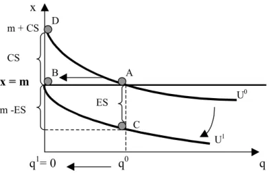
The geometrical representation of CS and ES money measures associated to the ecosystem

destruction is shown in Figure 1, where U1 < U0, x is the numeraire with a price of one (p = 1)

and the budget line is horizontal i. e. x = m. This means individual will spend all his or her

available income in x for every level of natural amenity q.

It is assumed that at given prices and income, the individual will always choose more of q if

given the option.

x

q

U0

U1

B A

C ES CS

m + CS

m -ES

x = m

q0 q1= 0

D

Figure 1 Compensating and Equivalent Surpluses for a loss in q from q0 to q1, where q1 = 0

In Figure 1 the point A is the initial consumption level of the individual, where he or she

consumes q0 and spend all his or her available income in x, and achieves the utility U0. The

decrease in q from q0 to q1 = 0 (because of the destruction of the ecosystem) enables the

individual to reach U1at point B. At B if income is increased by CS the individual is pushed

back to U0 but at point D compensating him or her monetarily for the welfare decreasing

associated with the destruction of the ecosystem (WTAC). Similarly, at A, if income is

reduced by ES, the individual is pushed to U1 at point C: the individual prefers to pay to avoid

the loss of welfare associated to the destruction of the ecosystem (WTPE).

Generally, WTA is different from WTP. Actually there is a substantial body of evidence from

both stated preference studies and laboratory experiments in evaluation that these differences

may be quiet large. Such discrepancies1 stem from the different welfare measure definitions

1 _{See Hanemann 1991 for more comprehensive analysis about the WTP and WTA discrepancy when applied to the valuation of}

and contexts of choice one has to deal with. The WTP economic value of an object of choice

is constrained by individual wealth and by the existence or non-existence of substitutes. These

constraints are not present in the WTA money measure. WTP and WTA are approximately

equal only when income changes, while (p, q) remain unchanged. When m0 changes to m1 =

m0 + ∆m the resulting CS and ES are equivalent and equal to ∆m. But for (p, q) changes,

WTP and WTA are different.

Randall and Stoll (1980) extended Willig’s analysis (Willig 1976) of welfare measures for

changes in q, to bound the differences between WTP and WTA. They found that, with some

alterations, Willig’s formulas could be used, by using information on the value of the price

flexibility of income over the interval [q0, q1]. Later on, Hanemann (1991, 1999) showed that

the price flexibility of income is the ratio between the income elasticity of demand for q and the aggregated Allen-Uzawa elasticity of substitution between q and x. If the elasticity of substitution is low, CS may be very different from ES.

Over the past fifteen years, considerable evidence has been accumulated regarding the

existence of some pattern of individual behaviour in judgement and choice involving

phenomena commonly known as loss aversion, endowment effect or status quo bias

(Horowitz and McConnel 2002). In short, the essence of these phenomena is that individuals

weight losses more heavily than comparable gains. As Kanemann and Tversky (1979) stated,

there is some evidence that individuals experience “loss aversion”, that is individuals may be

expected to value a unit of loss more highly than a unit of gain where he or she believes that

some right to the current amount of environmental asset exists.

WTP is only be equal to WTA where there is no income effect, where there are perfect

substitutes of the object under valuation and where the individual is neutral to losses and

gains.

WTP and WTA are though the fundamental monetary measures of value in economics for

market and non-market commodities and when economists set about measuring them they do

it by observing the preferences that individual have towards market and non-market

commodities. Standard theory assumes people have well-defined preferences over alternative

bundles of consumption goods, including non-market goods, and that people know their

preferences. Also it is theoretically assumed that preferences are non-lexicographic, in other

Preferences for private commodities are revealed directly by using actual, observed, market –

based information, at the very moment the individual purchases them on the market. But as

for the ecosystems because they are not market tradable, individual preferences have to be

elicit directly by simply asking people what is his or her WTP/WTA for a certain object of

choice – the preservation or the destruction of the ecosystem. Because people feel satisfaction

with ecosystems and the amenities they provide as reproducible natural asset, the ecosystem’s

economic value will be necessarily linked to the value of flows of services and passive use it

generates, at the moment the valuation question is being made. However, the ecosystem and

its components provide flows of services and of passive use over a time path and not only at

the time of the questionnaire. So, the value of the ecosystem accordingly to the asset analogy

will be equal, not to the sum of the individual stated WTP/WTA at the moment of the

questionnaire, but to discounted sum of the stated WTP/WTA over individuals for those

services and passive use benefit flows instead.

On using the natural asset analogy one must be aware that ecosystem’s changes depend on

changes in the quality/quantity of service flows and their passive use values; where there are

substitutes for ecosystem services, the TEV will respond to changes in that substitute; and that

TEV will depend on individual income constraint and methodological factors as well.

To estimate TEV one though has to go through the following steps: i) to estimate WTP/WTA

for an ecosystem that produce amenities by assessing the value individuals give to the

existence of that ecosystem after real responses stated by individual; ii) to estimate TEV,

using the aggregate values of stated WTP/WTA discounted for some rate, following the

natural asset analogy.

3. Estimating the Ecosystem’s TEV at Time t by Using Individual Stated Preferences

The Contingent Valuation Method (CVM)

Following the previous theoretical approach, let now q0 be a state characterised by an existing

ecosystem and q1 the one characterised by the loss of that ecosystem so that ∆U = U1 – U0 <

0. Accordingly to Mäller’s welfare measures for quantity changes, WTPE is the maximum

individual’s equivalent WTP to avoid that loss while WTAC is the minimum compensation he

Contingent Valuation Method (CVM) 1 provides the means to estimate WTPE and WTAC after

real responses.

Accordingly to CVM, by drawing a sample of people from a population, one simply has to

ask them about their maximum WTPE or minimum WTAC. WTPE is the more applied

measure because it overcomes the individual’s “risk aversion” related problems. The type of

population one has to consider depends on the ecosystem’s characteristics in terms of size and

ecological importance. These direct valuation questions permit to derive a set of welfare

measures wi (i = 1, …, n individuals) for the n respondents of the sample and for the moment

t, the moment the questionnaire is displayed where wi = WTPiE.

An estimate of TEV for the relevant population at the moment t can be obtained so that

TEVt = wt× N (10)

Where N is the population and wt is some mean estimated from the wi answers.

Three methods can be used (Freeman III 2003) to get the mean wt. It may be simply equal to

the sample mean w*. Or, alternatively, wt can be obtained as a bid function for the given

change from q0 to q1 by regressing the responses on income and other socio-economic

characteristics to obtain wt = wt (m, SE, P) where SE is a vector of socio-economic

characteristics of the relevant population; P is a vector of variables that measure the degree of

individual’s ecosystems perception that condition his or her attitudes towards ecosystem

conservation. A third approach is to obtain wtas a bid of a function as well, but by including

the q variation across the sample as part of the survey design, obtaining wt = wt (∆q, m, SE). This bid function can be estimated and then used to calculate the values associated with

different alternative scenarios regarding ecosystem changes2.

The Validity and Reliability of the CVM’s Estimates

The use of CVM to estimate the theoretical economic measures to quantify the TEV of

natural amenities, and specifically the WTPE to avoid the ecosystem destruction, has been one

of the most fiercely debated issues within environmental economic valuation literature over

the last twenty years. One of the main debated issues has been the validity and reliability’s

problematic of CVM’ WTPE estimates as the key to any evaluation method is that it must be

assessed in terms of how closely it represents an accurate measurement of the real value. The

1 _{For a detailed description of the CVM see Mitchell and Carson 1989. For a more theoretical detailed description of economic valuation}

methods see Freeman III 2003, or Braden and Kolstad 1991. See also Hufschimdt et al 1983. For examples of valuation methods applied to value ecosystem’s services see Goulder and Kennedy 1997. See also Carson et al 2003 for an elaborate and state-of-the-art valuation study.

closer the real values are to the estimated, the more accurate the valuation method is. If

WTP/WTA were observable there would be no problem. But given they are not, it is then

necessary to use other complex criteria and “rules of evidence” to assess accuracy. In

measurement, accuracy means the reliability and validity of data analysis used for the

valuation framework1.

From the economics perspective, reliability is related with the accuracy of aggregate WTP

over appropriately defined aggregates of individuals. Economists tolerate certain amounts of

unreliability in the estimated WTP, if random errors in measurement remain within tolerable

boundaries. Thus, the valuation technique reliability depends on the degree of data "noise".

The bias between the CVM estimated WTP/WTA and the theoretical WTP/WTA grows

where the former tends to systematically diverge from the latter.

The concept validity relates to the CVM application process. It involves numerous issues that

must be resolved mainly based on individual judgement of the CVM implementing entity.

Because WTP/WTA are not observed, inferences as to validity have to be based on indirect

evidence related both with the content validity of the CVM study’s design and execution, and

with the construct validity dealing with the degree to which the estimated money measure

relates to other theoretical measures. A number of guidelines have been developed to assume

CVM credibility, validity, and reliability (Portney 1994; Arrow et all 1993). The most

important are related to the presentation of adequate information over the object of choice (i.

e. the ecosystem2) and the context of choice3,the choice of a credible (hypothetical) payment

mechanism4 and the use of a referendum format5.

Detractors argue that respondents provide answers inconsistent with the basic assumptions of

utilitarian rational choice because of the embedding effect. The embedding effect refers to

several interrelated regularities in contingent valuation surveys like insensitivity to scale and

scope, sequential effect and sub-additive effect. Firstly, WTP is sometimes much less

dependent of the quantity of the public good provided that it should be theoretically

(insensitivity to scale and scope). Secondly when the several public good are valued in the

same survey, the WTP for a particular one often depends on its position in the sequence of

1 _{See Mitchell and Carson 1989 for a comprehensive description of these methodological CVM problems and their potential effect upon}

estimates and Freeman III as well. See also Jakobsson and Dragun 1996 for a comprehensive survey of literature on such issues.

2 _{The attributes of the ecosystem, the level of the provision of those environmental attributes “with or without intervention” and if there are}

undamaged substitute commodities. The researcher mustpreviously determine which attributes (services) affect the value an individual places on a good (Green and Tunstall 1999; Fischoff and Furby 1988).

3 _{To explain the extent of the market by informing respondents of how and when the environmental change will occur, as well as the decision}

rules in the use for such provision e.g. majority vote, individual payment.

public goods (sequential effect). Finally, the sum of WTP for individual changes often

exceeds the WTP for a composite change in a group of public goods (sub-additive effect).

Some CVM’s critics see the embedding effect as evidence for non-existent individual

preferences for the public good but an individual worm glow effect instead, created by the

survey process itself. Defenders acknowledge that early applications suffered from many of

the problems critics have noted (see Mitchell and Carson 1989); however, recognition is

required of how more recent and more comprehensive studies have dealt and continue to deal

with those objections (see Carson et all 2001).

More recently there has been a trend to include expertise from other disciplines such as

marketing research, survey research, and psychology (both cognitive and social) to improve

the CVM methodology both from the theoretical and empirical point of views. The

importance of these contributions to survey research is almost intuitive because CVM is

broadly survey valuation method based. Due to the hypothetical nature of the WTP question

asked together with the unfamiliarity of the task, one cannot exclude the possibility of

respondents to fail to consider the effect of their budget constraints and substitutes. Though,

symbolic valuation in the form of attitude expression and superficial answers are to be

expected (Kahneman et all 1999). Psychologists criticise the utilitarian approach1 because

they consider individuals do not chose in isolation but are affected instead by the

characteristics of their particular social–economic group; and they do not choose based on

only one restriction such as income. Preferences are not static and they are not equal across all

individuals. Psychologists criticise utilitarian economics for the assumption that all values are

commensurable and ultimately reducible to a single metric be it money or another type.

Psychologists defend CVM responses are sensitive to these methodological factors that in

standard economic theory are deemed irrelevant2. Underlying much of this discussion are

implicit assumptions of what Fischoff (Fischoff and Furby 1988) called the philosophy of

basic values.

Another capital issue of debate concerning the valuation framework approach of non-market

natural amenities has been the doubt with the inclusion or non-inclusion of passive users as a

1 _{See Green and Tunstall 1999 for a comprehensive introduction to the psychological perspective on economic valuation.}

2 _{This is the case of the so-called protest responses: i. e., protest bids (since zero to infinite bids), non-response, or unreasonable sacrifice.}

TEV component1. Many detractors of this kind of valuation framework generally argue that

passive uses cannot be seen, and though cannot be economically measured, as a simple

component of the economic total value. They claim that by the fact of being strictly associated

with ethical, religious principles, passive uses cannot be measured through WTP/WTA.

However, as far as the ecosystem’s valuation concerns, passive use will always implicitly

manifest itself if individual are willing to pay some amount of money to preserve the

ecosystem from typical economic activities, even though that individual is not an actual nor

intend to be a future user of the ecosystem’s services and would not suffered a utility

decreasing derived from the destruction. Passive uses do not complicate the valuation task at a

conceptual level and CVM seems to be capable of measuring TEV including passive use.

There is however some problems with passive uses if they exist for many other natural

resources at the same time and if they are widespread among the population. Being it so, the

valuation task will be more complicated, because a substantial surveying effort will be

necessary to get an accurate accounting for environmental amenities.

4. Estimating the Economic Value of Ecosystem as an Asset Using Individual Stated Preferences

The TEV estimated following the equation (10) is the aggregated welfare money measure of

the value the relevant population puts on the existence of an ecosystem, at the moment t. But,

as we already told, an ecosystem is a natural, reproducible asset that yields flows of goods and

services over time. And the measure given by (10) only reflects the value of the ecosystem’s

goods and services flow generated at the single moment t. One though has to consider the

temporal dimension of these flows.

The default criteria used by economists to include time is provided by the discounted

utilitarianism framework which until now has dominated more for lack of convincing

alternatives than because of the conviction it inspires (Heal 1998). It has proven particularly

controversial not only within non-economists concerned with environmental valuations but

also with some economists. We shall discuss this later on in this paper.

Following discounted utilitarianism approach (see Freeman III 2003 and Perman et al 2003)

let us assume a simplified intertemporal social welfare function of the type

W = W [φ1 U1 (x1, q1), …, φt Ut (xt, qt), …, φT UT (xT, qT)] (11)

Where the arguments are assumed additively separable, the single-period utility function

denoted φt Ut (xt, qt) is the same for all the periods, and the φt’s are weights used in summing

utility over generations to obtain a measure of intertemporal social welfare. The utilitarianism

approach to intertemporal questions typically assumes that:

φ : [φ1= ...; ρ + 1 1 φt = t ρ + 1 1

; … ; φT=

T ρ + 1

1

] (12)

where ρ is a subjective rate of time preference. If ρ > 0 we can write:

(

)

(

=

=

+

∑

t 1 1

W U x

1 T ,q

)

Whose continuous time version is:

(

)

=∞ ₋

=

=

_∫

t 0

W U x ,q e dt (14)

Let us now assume a marginal decrease in qt so that individual would be willing to pay a

quantity of the numeraire xt to avoid the loss in that period (WTPtE) or be willing to accept a greater quantity of numeraire in that period to held utility constant (WTAtC). The equivalent

compensated money measures of welfare change are equal to the marginal rate of substitution

between qt and xtso that:

( )

( )

W t t t

t t

x ,q _{t t}

t

U x ,q q MRS

U x ,q x

(15)

According to the first-order conditions to maximise the intertemporal social welfare function

given by the equation (13) (or (14)) subject to the wealth constraint1, where the individual’s

intertemporal marginal rate of substitution must be equal to one plus the interest rate, one can

say that, with intertemporal equilibrium, the individual would be indifferent between paying

an amount of money equal to t in period t to avoid the loss and paying

qt

W

(

)

t q 0

q ₁₊ρ

W = W t t in 1

(

)

(

)

= =

= = +

+ +

∑T t 0 ∑T T

t

t 0 t 1

1 1

x W* W m

1 1 t

, where W* is lifetime wealth and W0 _{the initial health. The individual can}

period 0, i. e. now. Or the individual would be indifferent between accepting the quantity of

money t now, to tolerate the loss of the ecosystem.

qt W t t q w

If the stream of future ecosystem’s service flow (let us say Q = q0, …, qt, …, qT) is expected to decrease, the marginal willingness to pay now to avoid the decreasing over the time path

( ), will be equal to the sum of the willingness to pay to avoid each of the components of

the decreasing; or the marginal willingness to accept a compensation to tolerate the negative

effects over the utility of that loss will be equal to the sum of the willingness to accept a

compensation to tolerate each of the components of the decreasing so that:

0 Q0 W

(

)

∑

∫

Q t t 0 q

t 0

w

W w

1

t

e dt (16)

where is one of the single-period welfare measures WTP E or WTA C.

Applying this intertemporal utilitarian approach to equation (10) we obtain the TEV of a

natural asset generating a flow of amenities over a relevant period of time T by simply

summing up the present value of the single-period welfare measures by using some discount

rate ρ1 so that:

ρ =

=

+

∑

t 0

TEV TEV

(1 )

(17)

whose continuous version is:

ρ

− =

=

_∫

TEV TEV e dt (18)

By considering these results, the typical practice in evaluating the TEV of some ecosystem as

an asset, that yields a flow of amenities over many years, is to estimate a single-period

welfare measure by using the CVM and to compute the present-value of this single-period

benefit using some discount rate. At a first glance, this seems to be a quite easy task.

However, although discounted utilitarianism approach has dominated, it has proven

particularly controversial when applied to environmental valuations. At origin of such

1 _{Nevertheless we can not say that compensate/equivalent welfare measures are equal to compensate/equivalent discounted single-period}

controversy are: the practice of the discounting, itself; the number used to measure the rate of

discount, ρ; and the irreversibility, risk, and uncertainty, surrounding the future outcomes.

5. Problems that Arise From the Consideration of Temporal Dimension

The time period and the positive rate of discount

A first target of criticism concerning discounting utilitarianism is the legitimacy it self of

applying discounting to the ecosystem valuations due to the very large period of time

involved. A positive utility discount rate forces an asymmetry between the evaluations of

current and future generations, particularly those very far in the future. The consideration of

an existing positive rate of discount is a way by which the market penalises investments with

long-term payoffs. This is precisely what happens when one has to value ecosystems by

discounting the flow of amenities they provide over time. At any positive discount rate, the

present value of any ecosystem is almost irrelevant due to geometric discounting and so it is

irrational to be concerned with extinction and conservation benefits. Economists face some

difficulties with valuing natural assets, because typical economic time horizons differ by an

order of magnitude from those that are typical for ecosystems. To economist 30 years is a

very long time. But to nature is a very short time.

It seems we have to deal here with some kind of a paradox. From one side societies are really

concerned with the social costs that will occur one hundred years or more ahead if ecosystem

depletion is to occur. From another side, the only convincing existing method to evaluate

intertemporal projects seems not to capture a very real part of society’s concern with the

future. The appliance of a discount rate to a future sum can make it look very small in

present-value terms when we are dealing with periods of 50, 100, 200 years or more1.

Some notable economists like Ramsey (Ramsey 1928) argued that applying a positive rate of

time preference to discount values across generations is “ethically indefensible”. They are

convinced that the only ethically defensible position in comparing utilities over successive

generations is to treat utilities equally, which means to make ρ equal to zero1. However, Heal

1985, 1998 demonstrated that discounting the future utilities is in some sense logically

necessary because without it a variety of non-setting inter temporal paradoxes can be founded.

He showed that Ramsey’s approach only works under some severe constraints, which in

general are not true. It can be proved that if t tends to infinity, as is the case of preserving

1 _{For instance if one discounts present world GNP over 200 years at 5% annum it would worth only a few hundred thousand euros today.}

ecosystems, the Ramsey’s approach provides incomplete rankings of inter temporal utilities.

Besides, a growing body of empirical evidence suggests that the discount rate that people

apply to future projects is positive, not zero, and depends on the futurity of the projects, and

on the magnitude of the income involved. Over short 5 years periods, individuals use discount

rates that are higher even then many commercial rate, around 15% and sometimes more. For

projects over 30-50 years the implied discount rate drops from about 5%, and down to about

2% for projects over 100 years2. Some defenders argue that the use of a positive discount rate

to discount the ecosystem conservation’s benefits is necessarily implied by the proper logic of

discounting utilitarianism and intergenerational equity3.

Discounting is controversial and so it is the arithmetic of discounting. The utilitarian

geometrical discounting based on a positive constant rate is discriminating against the future

generations, by giving their utility levels less weight. But empirical evidence seems to deny

the constancy of the discount rate. This put some economists4 to think over classical

utilitarian approach alternatives, particularly over those who place more weight on the future

then do the conventional one.

The logarithmic discounting (or hyperbolic discounting)5 is one of these alternatives. It is

grounded in the empirical individual behaviours, which suggest that a given change in futurity

leads to decreasing weighting of the future utilities, the further the event goes into the future1.

E. g. postponement by one year from next year to the year after is much more different from

postponement by one year from 50 to 51 years hence. The result is that the discount rate is

inversely proportional to distance in the future, which means one has to measure t in a manner

different from the one used in the utilitarian approach, by equalising proportional increments

in time rather then by equalising absolute increments. In this case, (17) and (18) will be

estimated by:

ρ ρ

− =

=

= =

+

∑

∫

t 0 log t t 0

TEV

TEV TEV e dt

(1 ) (19)

Where is a logarithmic factor of discounting. When t →∞, the discount rate and the

discount factor goes to zero in the limit. Unfortunately, as Heal 1998 noted, the use of a

t log ρ e

1 _{Harrod 1948 agrees with Ramsey’s opinion in the essential case of environmental subjects. In the particular context of global worming,}

Chine 1992 and Broome 1992 also argue for the use of a zero discount rate.

2 _{Cropper et al 1994; Lowenstein and Elster 1992; Lowenstein and Prelec 1992; Lowenstein and Thaler 1989; Thaler 1981.} 3 _{See also Baumol 1968.}

deterministic declining rate, though consistent with individual preferences, produces

time-inconsistent decisions.

Alternatives to use continuously declining rates are to simply use a lower rate for long-term

projects. Ramsey, as we already told, defended a zero discount rate although for certain cases

the zero approach provides incomplete rankings (when t → ∞) or even creates mathematical

problems like non-existing solutions, as it seems to be the case with the evaluation of pure

environmental depletion problems2.

Further later, economists tried to introduce other criteria like Overtaking’s, Limiting Payoffs,

and Chicilnisky’s criteria3 to avoid the problems arising from the appliance of a zero discount

rate and yet maintaining equal weight to present and future flows. The first two criteria are

criticised because they do not rank paths completely, they are neutral with respect to timing,

and neglect the present to over-emphasise the long run. The later, as demonstrated by Heal, is

a mixture of the discounted utilitarianism with the other two approaches. Chichilnisky

proposes to replace discounted integral of utilities by the following:

α ∞₌ α

→∞

∆ + −

∫

t

t lim t

t 0TEV (t) dt (1 ) TEV (20)

Where α ∈ (0, 1) and ∆ (t) is any measure of the discount factor that, in particular, could be

the conventional exponential factor , or the logarithmic factor of discounting, or

even the general non-constant factor discounting (like in the empirical case). This is, in effect,

a mixture of the other approaches. The left side of the addition is a generalisation of the

discounted utilitarian approach; and the right side represents the sustainable utility level

attained by the environmental related decision (see Heal 1998 for details).

( )t =e ρt

∆

-More recently Newell and Pizer 2003 described an alternative explanation of declining

discount rates that fits within the standard framework of geometric discounting based on

market-revealed rates. They introduced only one alteration in the geometric discounting

framework, by substituting a certain, constant discount rate, by an uncertain one. By doing so,

they claim there will be an increase in the expected net present-value of future payoffs.

1 _{For a comprehensive discussion over the rationales to adopt the hyperbolic discounting see Harvey 1994, Weitzman 1998 and Newell and}

Pizer 2003.

2 _{See Heal 1998 for a clear discussion of this issue.}

Irreversibility and Uncertainty

Beyond the controversy surrounding the discounting utilitarian framework and its arithmetic’s

some other important questions arise where ecosystem preservation is discussed like

irreversibility and uncertainty. With economic growth and technological change it is

reasonable to assume a tendency for the relative value of ecosystem services, i. e. the value of

scarcity, to increase (Krutilla and Fisher 1985). A way to introduce this into equations (17) e

(18) is to assume that preservation benefits grow at a rate a so that (and only for the

continuous version just to simplify):

(

)

− − =

=

_∫

TEV TEV e dt (21)

Generally the value assumed for a, is equal to the long-term rate of economic growth1,

because it is assumed by many as a plausible lower bound for the value a, should to assume.

This approach is similar to hyperbolic discounting.

Uncertainty is also an important characteristic faced by individuals who are users or potential

users of ecosystem amenities. They might be uncertain as to whether a specific ecosystem

amenity flow will be available for their use in the future; or whether individuals themselves

will want to use some ecosystems in the future or to give future generations the opportunity to

decide between conservation and development. These uncertainties will affect the welfare

measures and the calculation of TEV. One has to adopt the expected value of the TEV instead

the TEV as we did in (17) e (18).

Following Perman et all 2003 and Freeman III 2003, the measure of the Expected Value of

TEV [E(TEV)] with risk aversion (and for the continuous version only to simplify) will be

given by:

ρ ρ

− −

= =

=

_∫

_∫

t 0 t 0

E(TEV) E(TEV ) e dt OV e dt (22)

where OVt is the individual’s Option Value at time t that is the maximum amount the

individual would be willing to pay in each period t, for an option that would guarantee the

existence and the use of an ecosystem. OV is a risk aversion premium (Cicchetti and Freeman

1971) and, in principle, can be obtained directly from suitable application of the Contingent

What Rate of Discount Can be Used?

What number should be assigned to the rate of discount ρ? More recently Arrow et al 1996

advocate that there are basically two approaches to choose the discount rate, the prescriptive

approach and the descriptive approach. Under the former, lower future discount rates must be

used (tending to zero) in contrast with the last approach that relies fully on historical market

rates of return to measure the discount rate.

In practice, policymakers have, in some cases, applied lower discount rates to long-term

intergenerational projects (Bazerlon and Smetters 1999) but it seems this causes

time-inconsistency problems as we already mentioned. If one adopts the descriptive approach

instead, the discount rate is equalised to the market interest rate and (17) e (18) will be

re-written as follows:

− =

=

= =

+

∑

∫

t 0 t

t 0

TEV

TEV TEV e dt

(1 r) (23)

where r is the market interest rate.

However, there is a multiplicity of market interest rates. Such multiplicity is related with the

existence of transaction costs, market imperfections, differences in the tax treatment of

interest paid and interest received, and different risk degrees faced by individuals. The first

problem is related with the effect that taxes have on income. As a consequence, discounting

for welfare evaluation should be done at after-tax interest rate because an optimizing lender

will equate his or her intertemporal marginal rate of substitution to the after-tax rate of return

(Freeman III 2003). A second problem arises with inflation, though there is a universal

agreement among economists: they all agree in using real rates instead of nominal ones.

Overall, the evidence from financial markets suggests that the individual’s real after-tax of

interest lies in the range of 1% - 4% (Freeman III 2003). Finally, there is a third problem

which is that of individual facing different interest rates, and having different portfolios of

investment. How shall one deal with all these rate differences when we have a single-period

welfare measure that is aggregated across individuals facing different rates of interest? The

standard assumptions say to assume the risk-free market interest rate as a proxy for the

relevant market interest rate, that is, the interest rate on government bonds2.

1 _{To ecologists the efficient sustainable rate is equal to the growth rate of Net National Welfare (NNW) where NNW = GDP + Normal}

Market Output – External Costs – Pollution Abatement – Depreciation of Created Capital – Depreciation of Natural Capital (Goodstein 1999).

2 _{See Freeman III 2003 procedure for calculating aggregated values in the second-best situation, where individuals face different interest}

A major issue in the evaluation of ecosystem preservation has been: how to account the fact

that preserving some ecosystem is likely an impediment to make an alternative economic

investment that could generate a higher rate of return than the effective interest rate governing

individual’s intertemporal substitutions? In an ideal, theoretical world, there would be no

problem to choose the discount rate because it would be equal to the market interest rate and

to the investment rate of return. But, in reality, investment rates of return are, in fact,

generally higher and in some cases considerably higher than market rates of interest1. Which

of these two must be chosen?

Economists are divided. With the market interest rate individuals would be better off; but they

would have been even better off if the private project would go ahead2. Nevertheless, where

environment is involved, most non-economists (and some economists) take the view that the

lower rate is the more adequate to apply geometric discount, because it attaches more weight

to the interests of future generations than the higher one.

6. Conclusions and Final Remarks

In common usage, value means importance or desirability. To an economist, the value of an

ecosystem is related to the contribution it makes to human well-being. The utilitarian

approach allows value to arise in a number of ways depending on how individuals use

ecosystems. Ecosystems are natural capital, generally defined as the stock of environmentally

provided assets (e. g. soil, atmosphere, forests, water, wetlands, and minerals) that provide

flows of natural goods and services that are directly and indirectly appropriate by the

economic sector and society in general at free cost. Hence, economists have generally settled

for taxonomy of total ecosystem value interpreted as a Total Economic Value (TEV) that

distinguishes between Direct Use Values and Passive(Non-use) Values.

The economic value of an ecosystem thus relates to the TEV and is an answer, mostly

expressed in monetary terms, to a carefully defined question in which two alternatives are

being compared. Mäler stated that it was possible to build four measures of individual welfare

change associated to choices involving non-market goods and consequently involving

ecosystems too. If there is an improvement in utility the measures are WTPC and WTAE. If

there is a loss the measures will be WTPE or WTAC.

1 _{See Freeman III 2003 to a more comprehensive explanation about the implications of this issue over the discounting of benefits related with}

public investments in general.

To estimate TEV one has to go through the following steps: i) to estimate the WTP/WTA for

an ecosystem that produces amenities, by assessing the value individuals give to the existence

of that ecosystem after real responses stated by individual; ii) to estimate TEV, using the

individual aggregated value of stated WTP/WTA discounted for some rate, following the

natural asset analogy.

The use of CV methods to estimate the theoretical economic measures of TEV for

environmental services has been one of the most fiercely debated issues within environmental

economic valuation literature over the last twenty years. The main issues of debate are the

validity and reliability of CV estimates, and the inclusion or non-inclusion of passive users as

a TEV component.

The CV method allows getting an aggregated welfare money measure of the value that each

individual puts on the existence of an ecosystem, at the moment t. To calculate the

ecosystem’s value as an asset one uses, by default, the discounted utilitarianism framework by

simply summing up the present value of the single-period welfare measures. Although

discounted utilitarianism approach has dominated, it has proven controversial when applied to

environmental valuations, being the practice of discounting, the number used to measure the

rate of discount, the irreversibility and uncertainty, the main origins of that controversy.

Although there is controversy towards theoretical, methodological, and empirical aspects of

the ecosystem’s TEV framework one must not agree with the resigned argument that “a

number is better than no number”. Because when talking about economic values economists

are not referring to any number, but to a number rigorous theoretically defined and carefully

applied instead in order to capture the real value people put on the object of choice under

certain circumstances of choice.

Better then saying, “a number is better than no number” is to say “an economic number is

better as a minimum reference number, than any number at all. What we mean is that nobody

is defending that this economic tool should rule the day. Economic valuation is only one of

the criteria available to evaluate environmental policies and decisions. The utilitarian

approach allows value to arise in a number of ways depending on how society uses

ecosystems. And society includes individuals such as consumers, scientists, educators,

politicians, and stakeholders, like firms or non-governmental organisations. CVM is an

individual stated preference based technique used to estimate the TEV in a way consistent