ESTIMATING THE RECREATION VALUE OF
ECOSYSTEMS BY USING A TRAVEL COST METHOD
APPROACH
1Working Paper to be presented to the Permanent Seminar of the Department of Economics
24th May 2005
Isabel Mendes
Department of Economics
Instituto Superior de Economia e Gestão-ISEG/Centro de Investigações Regionais e Urbanas-CIRIUS/Technical University of Lisbon2
Isabel Proença
Department of Mathematics
Instituto Superior de Economia e Gestão-ISEG/Centro de Matemática Aplicada à Previsão e Decisão Económica-CEMAPRE/Technical University of Lisbon3
1 This is a first draft. Please do not quote without the author’s authorisation. 2
Rua Miguel Lupi, 20, 1249-078 Lisbon, Portugal; http//www.iseg.utl.pt; Tel: 351 21 392 59 67; Fax: 351 21 396 64 07;
Email: [email protected]. Financial support received from the Fundação para a Ciência e Tecnologia under FCT/POCTI, partially funded by FEDER, is gratefully appreciated.
3 Rua do Quelhas, 2, 1200-781 Lisbon, Portugal; http//www.iseg.utl.pt; Tel: 351 21 392 58 66; Fax: 351 21 392 27 81;
ABSTRACT
Recreation is one of the ecosystem’s secondary values of a well conserved natural
ecosystem, associated with the direct use individuals make of these natural assets. In
this paper we define and estimate the total economic recreation value to visitors of a
particular natural area, a national park. An on-site individual observation Travel Cost
Model, Count Data distributions, and a version of hyperbolic discounting framework
distribution were used to estimate a measure for the present recreation use of the site
and the total discounted recreation value for a 50 years period. The empirical estimates
of the average representative visitor’s present equivalent surplus willingness to pay,
based on the impact assumption of closure or loss of access to the park were 123 € per
day per visit, and 593 € per each average five days length visit, per visitor. These values
suggest that recreation use of nature has a higher value than certain economic activities
in the area.
JEL: C3; D1; D4; Q2.
1. Introduction
Increasingly, society is placing greater demands on wilderness areas for a variety of
products including biodiversity, wildlife habitats, and recreation opportunities.
Moreover, multiple-use sustainable management is been increasingly recognised as an
important environmental policy tool, while non-consumptive nature’s outputs like
preservation, wildlife, and outdoor recreation are required to be considered in resource
allocation decision-making on ecosystems. Hence, resource managers are facing
decisions that balance society’s different needs and values, while trying to ensure
ecosystem sustainable integrity. This commonly leads to conflict and litigation, as
individual’s and stakeholder’s opinions of ecosystem’s management are commonly
markedly different. Therefore managers need information that provides quantifiable
measures of individual preferences and values associated with different management
outcomes, to make effective, efficient, and equity planning and policy decisions. Money
metrics of ecosystem’s goods is though an important and desired tool in resource
management. This is particularly important in a world of limited financial resources
and environmental valuation, in combination with strong demand pressures for the
overexploitation and destruction of natural assets. Although environmental valuation
has been recognised and strongly applied by policy-makers in the EUA as an important
decision-making instrument in the early sixties (Loomis 1999), it was only in the early
nineties that EU environmental policies finally refer explicitly to economic valuation as
a tool of decision4. Theoretically the utilitarian approach allows value to arise in a number of ways depending on how individuals use ecosystems5. Henceforth the recreation economic value of an ecosystem is economically defined as the sum of the
net discounted values of the streams of the recreation services it offers. Depending on
the type of use society makes of ecosystems, economics have settled for a total
ecosystem value taxonomy interpreted as Total Economic Value (TEV) that
distinguishes between Direct Use Values and Passive (Non-Use) Values (OECD 1999;
4 Economic valuation is clearly mentioned as an important tool of the EU environmental policy in the following documents: Treaty
on European Union signed in Maastricht in 1992, article 130R(3); the Fifth EC Environmental Action Program 1992 (Towards Sustainability: COM(92) 23); Treaty of Amsterdam 1997; the European Spatial Development Perspective (ESDP) document; the Agenda 2000 document; the use of Strategic Environmental Assessment (SEA), regulation 2001/41; the White Paper on Environmental Liability (COM (2000) 66); the Decision about the Sixth Environmental Action Programme 2001-2010 (Environment 2010: Our Future Our Choice: COM (2001) 31), January 2001; the European Strategy for Sustainable World (COM (2001) 264).
5 Here interpreted as natural capital, i. e. a stock of environmental provided assets (e. g. soil, atmosphere, forests, water, wetlands,
Turner 1999; Daily 1997). Total Recreation Value (TRV)6 is one of the components of the TEV. Following the Hicks (1939) and Kaldor (1939) generic economic definition of
value, the marginal recreation value an ecosystem has to the ith individual that visits it, becomes the amount his or her would pay or be paid to be as well off with the
ecosystem to produce recreation and leisure activities7 as without it. Thus, recreation value is an answer, mostly, but not necessarily, expressed in monetary units to a
carefully defined question in which two alternatives – the availability of the ecosystem
to be visited and used or some amount of money – are being compared. Mäler (1971;
1974) defined four fundamental monetary measures of value of individual welfare
change associated to choices involving the quantity and the quality of non-market goods
and services8 that can be easily applied to the existence and availability of ecosystems to produce outdoor recreation activities after the ecological characteristics of their
amenities. If the object of choice generates an improvement in individual (visitor)
wellbeing (a rising utility), like the availability of ecosystems for recreation purposes or
an improvement of the quality of the natural amenities two situations are possible.
Either the visitor is willing to pay (WTP) an amount to secure the change, termed
Compensated Willingness to Pay (WTPC) or he/she is willing to accept (WTA) a minimum of compensation to forgo it, the Equivalent Willingness to Accept measure
(WTAE). If the object of choice generates wellbeing deterioration (a decreasing utility) like the non-availability of some previous available ecosystem to be visit for recreation
purposes, or its simple destruction, two situations are again possible. Either the
individual is WTP to avoid this situation, termed the Equivalent Willingness to Pay
measure (WTPE) or he/she is WTA compensation to tolerate damage suffered, the Compensated Willingness to Accept (WTAC). Formally, the measures can be defined in terms of the visitor expenditures function as follows9:
(
) (
)
1(
)
0
0
1 0 0 0 , ,
/ , , , , r
C C
r
e p r U WTP WTA CS e p r U e p r U dr
r
∂
= = − =
∂
∫
(1)And
(
) (
)
1(
)
0
1
1 1 0 1 , ,
/ , , , , r
E E
r
e p r U WTP WTA ES e p r U e p r U dr
r
∂
= = − =
∂
∫
(2)
6
The formal definition of TRV and its components is based on Mendes 2004.
7 E. g. camping, hiking, sight-seeing, canoeing, birds- watching, horse-riding, climbing, and so on.
8 These four welfare measures were first proposed by Mäler as an extension of the standard theory of welfare measurement related
to market price changes formulated by Hicks (1943). The analysis of this type of problem involving changes to either the quantity or quality of non-marketed environmental goods and services rather then changes to price or income, is often referred to as the theory of choice and welfare under quantity (Johansson 1987; Lankford 1988).
CS and ES are Consumer Surplus and Equivalent Surplus hicksian welfare money
measures respectively, where r is a non-marketed environmental amenities vector representing an ecosystem and is assumed as a public good i.e. r is given;
(
1)
, ..., i, ... n
p= p p p p
0
r
0
is a vector of prices of the n marketed commodities that
maintains constant; is the initial state of r, characterised by the preservation of a healthy ecosystem that produces amenities and is the final state characterised by the
ecosystem destruction or the non-availability of a previous existent ecosystem for
recreation; U is the visitor’s level of welfare if he/she wishes to choose and U is the
visitor’s level of welfare if he/she chooses so that U U
1
r
1
r
0
r 1
1< 0
;
(
, ,r)
r ∂
P
t
U
/WT
e p
∂ is the
derivative of the expenditure function with respect to r, where t = 0 refers to the initial level of utility and t = 1 to the final’s, after the change in r; such a derivative represents the marginal value of a small change in r and is equal to the income variation that is just sufficient to maintain utility at its initial level (in the case of the CS money measure, t =
0) or final level (in the case of ES money measure, t = 1)10. Generally WTP differs from WTA which stems from both the respective differing welfare measure definitions and
the choice contexts (Hanemann 1999): i) WTP is constrained by visitor wealth and the
existence of substitutes as well, but WTA isn’t; ii) if (p,r) changes and the visitor available income m remains unchanged, the measures are different; iii) WTA is
particularly vulnerable to some pattern of individual behaviour in judgement and choice,
involving phenomena commonly known as loss aversion (Kahnemann and Tversky
1979), endowment effect or status quo bias (Horowitz and McConnel 2002). This are
the reasons why WTP is more often applied then WTA in empirical studies of
non-market valuation because it overcomes the visitor’s risk aversion related problems and
is limited by the visitor available income. In short, when an economist is talking about
the value the representative visitor gives to the right of using an ecosystem to produce
outdoor recreation flows at time t, he or she means to WTPCt /WTACt or WT Et AEt.
In the absence of markets, methods like Contingent Valuation, Hedonic Approach, or
Travel Cost are used to generate welfare outdoor recreation measures (1) and (2) for a sampled representative visitor based on a sample of n visitors selected from the N
10 The signs of the measures (1) and (2) depend on the change of r being an improvement or a loss. When ∆ is a hypothetical or
effective loss as it is in our case, then , and (- ES) measures the visitor’s WTP r
1 0
0
U U U
∆ = − < E to avoid the loss, while (-
relevant population. Aggregating this set of individual welfare measures across all the
individuals assuming that all behave like the representative one, then
0 0
0 Ct N Et N
t
S S
T R V = = W T A = × o r W T P = × (3)
and one gets the aggregated welfare money measure of the value the relevant population
puts on the availability of the ecosystem for recreation at the moment t = 0, the present
moment, to which one is trying to estimate the value. But, as already stated, being
natural reproducible assets, the ecosystems yield flows of recreation services over
several time horizons whose order of magnitude goes far beyond the typical economic
ones (30, 50, 100 or even 300 years and more) and the measure (3) only reflects the average present recreation value at a single moment t = 0. Applying the inter-temporal
utilitarian approach (Freeman III 2003; Perman et al 2003), we may obtain a money
measure of the ecosystem’s TRV that generates a flow of recreation benefits over a
period T by simply summing up the present value of the single-period welfare measure
(equation (3)) using a discount rate ρ11 so that
0
0 (1 )
t T
t t
T R V T R V
ρ
=
= =
+
∑
(4)The objective of this paper is to estimate the TRV as defined by (4) of a particular set of ecosystems, the Peneda-Gerês Natural Park (PGNP). To fulfilled this objective, the
following steps have to be taken: i) to estimate WTPEt0 /
s WTA
0 t
C s
= = for the NPPG by
assessing the average value that the sampled representative visitor gives to the existence
of the Park at t=0, and per each day of use; and ii) to estimate TRV using (4). To calculate WT we shall use one of the TCM’s individual based observation
versions and the demand recreation function will be estimated with count data models.
To our knowledge and at the moment we are writing the paper, there are no studies in
the professional literature dealing directly with the TRV, the recreation demand, or the
use of count data models to estimate the recreation use values afforded by the PGNP.
Within EU, many studies have been implemented since the last decade of the 20
0 / t
E S
P = WTACt0
S
=
th
century, to estimate the use and the non-use values of ecosystems, but only eight used
travel cost method (Navrud and Vägues 2000; Mendes 1997). Of these, only two
concern the PGNP (Mendes 1997; Santos J.M.L. 1997) and only one uses the travel cost
11 Nevertheless we cannot say that welfare measures at moment t = 0 are equal to discounted welfare measures for some ρ. This
method (Mendes 1997). The paper is composed of four sections. Following this
introduction, in section 2 we estimate the PGNP’s TRV for the sampled representative
visitor per each day of visit and per each average on-stay length visit. Count data
models will be used within a TCM framework to estimate a recreation demand function
of the park and the visitor surplus per day and per visit. The visitor surplus will be used
afterwards to estimate the theoretical individual welfare measures as defined by (3). In section 3 the TRV as defined in (4) is calculated, and in section 4 come conclusions and results discussion.
2. The Estimation of the PGNP’s Present Recreation Value for the Representative Visitor
Method
TCM provides a mean to estimate the monetary values of non-marketed commodities
based on actual behaviour, by using the individual’s expenses with marketed
commodities that are weakly-complementary with the non-marketed ones12 as an indirect way to reveal individual’ preferences (Freeman III 2003).The method
establishes a relationship between the costs (price) incurred by travellers to a site and
the number of trips taken. This relationship is further exploited to derive Marshallian
CS for access to the site, for a recreation experience, by simply integrating the area
under the demand recreation curve, between two levels of price (costs): the actual and
the choke price (cost). TCM is one of the more popular revealed preference based
method used in non-marketed valuation, over the past 30 years (Ward and Beal 2000).
The general theoretical basis derives from the basic economic notion of an individual
utility function subject to budget and time constraints. The representative visitor or
household preferences are represented by the utility function
( , , )
U =U x r q (5)
where x is a vector of market goods and services quantities, including those related with
recreational outdoor activities; r is a vector of recreational services including recreation
) 12 Let ( , ,
1 1
in the PGNP; and q is a vector denoting the quality characteristics of the ecosystems,
including the PGNP. The representative visitor is subject to two constraints: the budget
and the time constraint. The income constraint is represented by the equation
'
W X r
m=wT = p x+p r' (6)
where m is the available income of the visitor; w is the market wage rate; T is time
spent on work;
W
X
p is the price vector of the quantities x; and pris the price(cost)
vector corresponding to the quantities r. The time constraint is represented by the
equation
W
T =T +Tr (7)
where T is the total available time and T is the time spent with recreational activities r.
The representative
r
recreationist maximizes (5) subject to (6) and (7), yielding a set of ordinary demand functions for the marketed commodities and the recreational activities.
Thus, the ith recreationist’s demand function for the PGNP is
(
, , ,)
i r X r
r =g p p m q (8)
The estimated coefficients of (8) are further used to calculate the recreation value of the site. By simply integrating the recreationist’s demand curve between two prices (costs)
yields the CS marshallian welfare measure:
(
0
, , ,
r
r
p
r X r p
CS =
∫
g p p m q dp)
r (9)where pris the present recreation price which is equal to the recreationist’s total
expenditures necessary to produce r, and they may include trip, on-site expenditures,
and the opportunity cost of time; is the choke recreation price. The measure (9) is the money measure of the i
0
r
p
th
individual’s benefit related with the use of the site to
produce recreation activities. TCM allows to measureprin the absence of recreation
markets. The wide variety of TCM models appearing in the academic and empirical
literature are variants on the general structure of the model above, the way the
dependent variable r is defined and measured, and the estimation strategy used (Ward
and Beal 2000; Fletcher et al 1990). Building on the belief that the basis for evaluation
is the benefit measured by CS derived by people when they use the ecosystem, TCM is
predicated on a number of assumptions, foremost of which is that individual’s
recreation visits to a site respond to changes in the travel-related component of the cost
admission fee (Freeman III 2003). TCM has generally been preferred to estimate
economic use values over other non-market methods because of its behavioural base,
although is not free of limitations. In spite of its direct link to actual visitor behaviour, a
number of assumptions13 and research judgements are required to get from reported visits to the relevant economic measures, like elasticity of demand and CS (Ward and
Beal 2000; Mendes 1997; Fletcher and al 1990). The most frequently used TCM
empirical versions are the zonal and the individual versions. The zonal version of the
model was the first one to be developed (English and Bowker 1996; Hellerstein 1991).
It establishes a relationship between per capita participation rates (the recreation
demand r) at an ecosystem from various geographic origin zones, and the costs incurred
in travel (the price per each unit of recreation demand) from the origin zone to the given
natural site. The individual TCM version is conceptually similar to the zonal one,
however, the recreation demand/price recreation cost relationship is based solely on
individual observations. The individual version is highly preferred to the zonal for
reasons such as (Mendes 1997): i) statistical efficiency; ii) theoretical consistency in
modelling individual behaviour; iii) avoiding arbitrary zone definitions, and iv)
increasing heterogeneity among populations within zones. There are however several
problems with the nature of the dependent variable and the way it is measured and
defined. Demand for visits to a specific site is frequently measured in number of trips or
days per period of time. So they are non-negative integers which results in a truncated
(at zero) data set. A second feature of recreation demand data is when the dependent
variable is the count of the number of visits taken over some period of time (a season, or
a year), many observations near 1 or 2 are common. Therefore the observed dependent
variable is the outcome of a data-generating process based on unknown probability
distribution function defined on the non-negative integers, termed count data process. A
third feature of recreation demand is that with on site surveys of recreationists the
probability of some visitor being surveyed depends on the frequency of visits to the site.
This is called endogenous stratification. Count data models explicitly recognise the
non-negative discrete nature of the recreation dependent variable, and they are particularly
suitable for modelling recreation demand through the individual TCM version. A
number of recent studies applied this type of models to recreation demand. Shaw (1988)
13 Several separability assumptions are made concerning the arguments of the utility function like: i) the recreation activities used to
was the first to recognise the non-negative integers, truncation and endogenous
stratification nature of on-site sampling recreation data characteristics, and to assume
that the use of common regression linear methods with this type of data sample generate
inefficient, biased, and inconsistent estimations. He developed a standard basic Poisson
model (POIS) that corrected for the sampling problems. The basic POIS captures the
discrete and nonnegative nature of the dependent recreation demand variable and allows
inference on the probability of visits occurrence. However POIS estimators are biased
downward and Marshallian’s CS as calculated by (9) will be overstated in the presence of over dispersion14, a very frequent statistical phenomenon in real data. The standard negative binomial model (NB) corrects for over dispersion, by allowing the conditional
variance to be different from the mean (Long 1997; Grogger and Carson 1991).
Subsequent work has extended Shaw’s application to include truncated POIS (TPOIS)
and NB distributions (TNB), as standard POIS and NB estimators are biased and
inconsistent in the presence of truncation because the mean function of the count data
model is misspecified (Creel and Loomis 1990; Grogger and Carson 1991; Gurmu
1991). Further more, Gurmu and Trivedi (1994) noted that empirics demonstrated that a
vast majority of the visitors make at least one or two trips and the number of
recreational trips higher then two falls rapidly when the dependent variable is measured
in number of trips to the site. This is called a fast decay process, a common
characteristic in recreation-demand setting, and results in over dispersion. Sarker and
Surry (2004) proved that the NBII model is capable of fitting a fast decay process.
Englin and Shonkwiller (1995) developed a TNB model that corrected for both
endogenous stratification and truncation. To recent developments in count data models
applied to recreation see Sarker and Surry (2004) and Santos Silva (2003; 1997). Those
further applying count data models to recreation demand functions and related welfare
estimations based on individual TCM version include Hellerstein (1989; 1991), Creel
and Loomis (1990; 1991), Hellerstein and Mendelsohn (1993), Yen and Adamowics
(1993), Bowker and Leeworthy (1998), Sarker and Surry (1998; 2004), Crooker (2004);
Englin and Moeltner (2004). Finally, the second problem with the nature of the
dependent variable is related with its definition. If demand is defined as the number of
trips to a site during a period of time, we will be dealing with a non-homogeneous
14 There is over dispersion when the conditional variance of the dependent variable is greater than the conditional mean. This
dependent variable, because there are one-day trips, two-day trips, three-day trips, and
so forth. Non-homogeneity of the dependent variable becomes particularly problematic
if the objective is to quantify monetarily welfare measures by using the CS measure,
because we are not considering an homogeneous marginal CS. This problem is not
generally recognised in most of the empirical TCM studies, even in those interested in
the calculation of welfare measures and not only in the study of the recreation demand
behaviour of a given site. One alternative to go beyond this obstacle is to define visits as
the number of days per trip instead of the number of trips or visits and thereby we can
calculate an average marginal CS associated with the recreation benefit of one day of
stay in the site15.
In this paper we want to monetarily estimate the recreation use value of the
representative visitor of the PGNP by using the WTPE welfare measure of one-day-of-stay in the park per visitor, by using the on-site individual TCM version to specify the
recreation demand function. We are not interested in recreation demand prediction. A
recreation demand function of the type of (8) will be estimated using count data models, in order to calculate the Marshallian welfare measure (9) for the sampled representative visitor. The measure (9) is equal or at least is a proxy of the true welfare Hicksian
measure WTPE only if the income effect related with pr is inexistent or very small16. If the PGNP’s recreation demand is a normal good, the hierarchical relation between the
three welfare measures will be WTP in the case of a decreasing utility,
related with the PGNP visitor interdiction. E
CS WTA
< < C
The Model
Although the recreation demand for a site may be modelled as aggregate or market
demand, the most common practice is to estimate the recreation demand of the
representative individual and then to calculate aggregate value measures as the sum of
the individual’s recreation values (Freeman III 2003). To estimate the marginal CS of
the ith PGNP visitor who seeks this natural site to enjoy its unique and rare natural
15 CS per day of use (CSPDU) is a common way to measure the recreation benefits the representative visitor derives from a visit and
is commonly used, for instance, by the US Forest Service as a basic recreation site value. Morey (1994) defined CSPDU and how compensate valuation can be derived from it. He proofed that CSPDU for a price change of a recreational site is that price change, so it is a constant, independent from the number of days the site is visited. And if it is a constant, it can be used, along with information on the number of days at the site in the initial and the proposed states to approximate for compensated CS for that change.
16
amenities and landscapes, by self-producing several recreational activities like camping,
sight seeing, hiking, canoeing, and others, we used an on-site individual TCM version
(Bell and Leeworthy 1990; Hof and King 1992; Font 2000), where the dependent
variable is number of days on-site, not number of trips, and because it uses on-site and
travel out-of-pocket costs, as well as travel and on-site time opportunity costs, and not
only travel costs. We used Mendes (1997) on-site TCM empirical approach, where the
representative visitor combines time and money to reach the site and to stay there, and
chooses the number of days per visit that minimize total travel and on-stay costs
(Wilman 1987).
The general specification of the TCM was
(
; ; ,)
i i i i
DRP = f price available recreation income individual characteristics β ε, i (10)
where price/recreation costs, available recreation income, and individual characteristics
are independent variables, β is the vector of parameters, and εi is a random
disturbance that is independent from the disturbances of other individuals. The
recreation demand was modelled as the number of days one visitor stays in the park, per
trip (DRPi ) at the time of the questionnaire. Count data models stipulates observed
individual days of recreation per trip as realisations of unobserved actual on-site
demand per trip, which follows standard or truncated POIS or NB distributions with
meanλi17. By choosing the semi-log form18, the expected on-day site demand equation
(10) is specified as follows:
(
0 1 2 3 4 5 6)
( i) i exp i i i i i
E DRP = =λ β +βCDRP+β YR +βTR +β ID +β ED +β Pi
6 i
(11)
and may be written as:
0 1 2 3 4 5
lnλ βi = +βCDRPi+β YRi+βTRi+β IDi+β EDi+β P19 (12)
where CDRPi, YRi, TRi, IDi, EDi, and Pi are explanatory variables, and β’s are the
unknown coefficient to be estimated. Explanatory variables include the ith minimum recreation cost of each day of stay in the PGNP, including travel cost (CDRPi), per
capita available recreation income (YRi), number of available days to spend with
recreation (TRi ), age (IDi), level of education (EDi), and the perception degree the
visitor has of the natural characteristics of the park ( Pi). As shown in Hellerstein and
17 See Appendix.
18 The semi-log form is commonly used to specify count data recreation demand models (Shaw 1988, Grogger and Carson 1991;
Long 1997).
19 Like many researchers in the past, Mendes (1997) used OLS to estimate several linear and non-linear recreation demand
Mendelsohn (1993), the representative visitor’s CS per each average day of stay visit
can be derived by integrating the recreation demand function (11) over the relevant price/ on-stay cost change i.e.
0
1 S
CDRP
S per visit CDRP S
CS λ dCDRP λ
β
=
∫
=− (13)where CDRPS is the actual sample mean of each day on-stay cost and CDRP0 is the
choke recreation day cost. The CS per visitor per each day of visit is simply measured
by
1
1
β
− (Bokstael 1987). Equation (11) gives λi, the expected latent quantity demand,
where β’s are the parameters of the population recreation demand for days of stay in the
park per visit. Therefore the respective estimates can be used to calculate the CS for the
general population (Grogger and Carson 199120; Englin and Shonkwiller 199521).
As shown in Bockstael et al (1987) and Englin and Shonkwiller (1995), the visitor’s
Hicksian welfare measures of one average length day-of-stay visit with a
semi-logaritmic form demand function, are given by the formulas:
2 2 1 1 ln 1 C S S
WTA λ β
β β
= +
and (14)
2 2 1 1 ln 1 E S S
WTP λ β
β β
= − −
where β1 is the estimated parameter of price/recreation cost of the recreation demand
function, and β2 is the estimated available recreation income parameter of the same
function. These expressions are based on the impact assumption of a recreation cost
change for infinity of a day-of-stay in the PGNP, which in turn can be interpreted as
PGNP closure or loss of access for the time period of interest. The expressions can be
converted into per-day of stay measure by dividing them by λS.
Aggregating (13) and (14) by (3) for the n individuals of the sample, yields TRV , the present recreation valuefor the sample
0
t=
22
.
20 “From equation (19) … we see that the effect of a change in one of the X
ith on the latent dependent variable in the full underlying
population can be inferred from information obtained from a choice-based sample [that is the group in the population of interest from which the choice-based sample is drawn]”, pp 6.
21 “The average person’s total use value is the product of the value per trip to the average individual in the population times the
number of trips the average person will take (the latent variable)”, pp 1.
22 Farber et al (2002) pointed out that this traditional aggregating visitor values procedure is an appropriate way to represent the
The Data, Estimation, and Analysis of Results
PGNP was created in 1971 and is located to Northwest of Portugal. It includes a surface
of 72000ha and it is the only National Park Category within the Continental part of the
country. It is an Area of Special Birds Protection and a site included in the National List
of Sites (Net Nature 2000). The park is rich in rare botanical species (as the lily of
Gerês, an Iberian endemism, or the fetus of Gerês) and it presents important stains of
well conserved oak-groves, riparial vegetation and peat-bogs. The fauna is also very
rich and includes the wolf, the stag, and savage ponies, several species of bats, and
Iberian Peninsula typical mountain birds. The area is fertile in prehistoric and Roman
trucks, medieval monuments, curious mountain agglomerates, and curious and unique
humanised landscapes like lameiros and prados de lima. Like many other European
national parks, PGNP experiences uneven recreation demand, with a peak period during
summer (July, August, and September), but it is during August that recreation demand
rises exponentially. The rest of the year is non-peak period. There aren’t available
statistics accounting for and characterising the visitors. The only existing data are those
of park’s camping sites, but they are not sufficient enough to characterise recreation
demand.
Some of the data used to quantify the dependent and independent variables of (11) were obtained part from an on-site inquiry by questionnaire to a population composed of
Portuguese citizen’s over-18th. 1000 questionnaires were distributed to Portuguese citizen’s over-18th that were visiting the park at the time of the questionnaire during the 1994 summer peak-period months, for visits equal or greater then 24h. 243 had been
correctly filled out. All the monetary data are measured in 2005 euros. The information
gathered included the number of days of stay in the park during that visit, the income
step the inquired belongs to, his/her geographical origin, the transportation mode, if
he/she travelled in company, various demographic characteristics (gender, age, number
of years of education, if they were in the vacancy period and the number of vacancy
days), and some questions to capture the visitor’s perception concerning the specificities
of the PGNP natural and humanised ecosystems and landscapes. Unfortunately we had
to drop this last variable because a great majority of visitors did not answer adequately.
Nevertheless, the questionnaire implemented by Santos J.M.L. (1997) permits to
conclude that visitors generally recognise the PGNP’s specificities, and their demand is
unambiguously related with them. Yet the absence of a perception variable in this
empirical on-site cost TCM approach is by no means an obligation, because the aim is
to estimate a welfare measure and not to predict multi-site or PGNP recreation demand,
nor to measure the welfare impact of quantity modifications in the ecosystems.
Substitutable variables are not considered because: i) we do not want to predict PGNP
recreation demand; and ii) one assumed visitors recognise PGNP as being a unique
ecosystem, with non-substitutable amenities. To overcome the multi-destiny trip
problems, trips to additional sites were counted as separate observations and thereupon
we considered visitor’s geographical origin to be the place the visitor was when he/she
definitely decided to travel to the park. To quantify the PGNP’s welfare measure, only
the relevant expenses strictly related with the trip and the on-site stay were considered.
For these reasons, the distance in Km’s since the origin to the site was calculated
assuming the faster and more accessible itinerary, to avoid the trip’s utility generation.
The Km’s were counted on a common road map. In the case of multiple destination
trips where the PGNP was not the primary purpose, only the round-trip km’s from the
temporary origin to the park was included23. To avoid lodging’s utility generation, camping was considered the relevant mode of lodging. Due to severe time and budget
constraints to implement the questionnaire, the camping on-site sample was the method
chosen to gather a sample with non-zero answers, and guarantee an adequate number of
observations related with one-day and more day visits. To avoid endogenous
stratification, visitors were interrogated at the time they addressed themselves to the
camping reception centre, for camping inscription. The cost of one day of stay24 in the park (in euros) was calculated according to the formula
i
i i vi ei
i
CV
CDRP CMDE CT CT PUD
MDE
= + + + +
23 Although this method used to surround the multiple destination trip problems remains a debatable researcher judgement, as all the
others do too, we feel, like Bowker and Leeworthy (1998), it is appropriated.
24 The marginal cost of one day of stay was assumed to be constant, which seems to be reasonable because: i) the travel cost is fixed
where CVi is round travel cost in euros25; MDEi is the mean number of days that the visitors with origin from the same geographical district as visitor i, stayed in the park26;
CMDEi is the cost in euros of each day of stay27; CTvi and CTei are the opportunity costs in euros of travel and on-site stay time per visitor per day, respectively; PUD is the park
entrance fee in euros which is zero. To quantify CTvi and CTei28 we partially based on
the opportunity travel and on-site time cost’s valuation method more commonly used in
TCM literature, where travel and on-site time cost is one-third of the individual’s wage
rate (Bockstael 1987; Chakraborty and Keith 2000)29. Instead of individual’s wage rate we used the visitor’s per capita per hour available recreation income measured in euros
instead. Travel and on-site recreation time were both previously estimated, and it was
assumed that a recreation day is equal to 16h following the definition of one typical
recreation day of Walsh (1986) ( see Mendes (1997) for details). YR, was estimated
since the net income declared by individuals in the questionnaire and it was assumed to
be equal to a 14th monthly remuneration (see Mendes (1997) for details). The other explanatory variables like TR, ID and ED were quantified directly from the
questionnaires. The sample has nonnegative integer characteristics, is truncated at zero
because observations with zero days in the park are not observed, and is not
endogenously stratified.
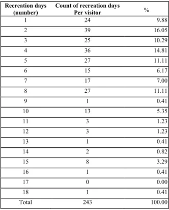
Descriptive statistics from the data set are presented in Table 1andTable 2. During the
on-peak summer season, the visitors of the PGNP stayed in the park for 5.284 days on
average. The data do not exhibit a quick decay process; more than one half of the
sample visitors took visits of one day to six days. About 10% took one-day visits, 16%
two days visits, 10% three days visits and so on. About 5% made ten days visits and 3%
fifteen days visits. The variance of the dependent variable is high, 12.766, which means
the equidispersion property of the POIS model may not hold. Table 3 presents the
]×
25
The transport mode was considered. If the visitor used a car then ; per-km cost was dependent of the technical characteristics of the vehicle and included oil, gas, and tolls. If the visitor used a moto, then
[
, cos / º ' 2
car per capita
CV = t km×n km s+taxes
[
cos / º ']
0.5 2moto t km n km s
CV = × × × . If
the visitor used a public transport, thenCVpublic =
[
travel fee]
×2. For individuals travelling together, shared costs were apportioned to the respondent. See details in Mendes (1997).26 The correlation coefficient between the distance travelled and the on-stay number of days is significantly inferior to the unity
( ), which allow us to assume the exogenity of the variable MDE with reference to the distance travelled (Rockel and Kealy 1991).
0 04. r=
27CMDE= camping visitor fee + car fee + alveolus fee. Food expenses are not included, because they are not relevant costs. 28
1 / 3
vcar
number of hours traveled to the PGN P and back CT median YR percapita perhour
number of days of stay
= × ×
;CTe=1/ 3×medianYRpercapitaperhour×16h.
29 The opportunity cost of travel and on-site time has been one of the more discussed issues by those economists interested in the use
parameters estimates from six specifications of count data model: standard and
truncated POIS, NBI, and NBII. The technical description of these statistical analyses is
found in the Appendix. We tested for several alternative specifications of the demand
equation (12)30 but the one that fits the best to the data is the semi-log form, which is presented. We also test for other two alternative methods of quantifying the travel and
on-site cost of time31, but the estimated price/recreation cost coefficients were all very similar, which allow us to conclude that our estimated demand recreation function is not
significantly sensitive to the way time cost is measured. The maximum likelihood
procedure is used to estimate all count data models32. It was hypothesized that demand for recreation days in the PGNP would be negatively correlated with the on-site daily
recreation cost and with age, and positively correlated with the available recreation
income, the available time for recreation activities, and the level of education. α, the
nuisance parameter, that reflects the existence of over dispersion, is significant in the
NB models, which suggests that the POIS estimation is not a suitable estimator for our
data33 given that it is truncated. This confirms our early conclusions drawn from the analysis of the descriptive statistics presented in Table 1. Furthermore, based on the
smaller value of the log-likelihood function of TNBI relatively to TNBII we may
consider the first a better fit. The standard errors of the coefficients were computed
using the Eicker-White procedure34. The price/recreation cost, the available recreation income, and the available recreation day variables have the expected signs. The
expected number of recreation days spent in the PGNP per trip goes down with higher
recreation costs and up with higher available recreation income and recreation days.
Therefore PGNP’s per trip recreation days demand is an ordinary (price-elasticity is
negative), and normal good (income elasticity is positive and inferior to one). Also, the
number of recreation days is more responsive to price changes than to income changes
(the absolute value of the price-elasticity is higher than the absolute value of
income-elasticity). Truncation did not reduce, rather augmented, the absolute values of price and
income elasticity. However, the demand for recreation days seems to be not very
30 Logarithms of continuous right-hand side variables and quadratic forms for some variables like ID and ED did not visibly
improved the results.
31 We test the results without time cost and with time cost equal to 50% of the median YR per capita per hour. And the results for
the parameter β1 associated to the variable of price/recreation cost CDRP varied between 0.00470 without any time cost, 0.00567
with time cost equal to 1/3, and 0.00550 with time cost equal to 1/2, for the NBII model. The same type of conclusion was drawn from the POIS and NBI models.
32 The estimation programs were written in TSP.
33 Over dispersion tests for the POIS regression confirm the evidence of over dispersion. 34
sensitive (inelastic) both to recreation cost and income variation; per each unitary
growth of recreation cost the demand for recreation days in the PGNP goes down only
from 0.53% minimum in the NBII distribution, to 0.72% maximum in the TNBI
distribution while per each unitary growth of the available recreation income, the
demand for recreation days goes up from 0.030% minimum in the NBII and TNBII
distributions to 0.04% maximum in the TNBI. Using TNBI estimates of price elasticity
(Table 3), a price/recreation cost increase of 1% per person per day effect approximately
a 0.364 drop in recreation’s day demand per person. The variable Age (ID) has the
expected signs, but the variable Education (ED) doesn’t. These two demographic
variables are the only ones that are not significantly different from zero. This is
explained perhaps by the fact the sample’s dimension is not sufficiently high to
incorporate the ID and ED variations as being significant for the DRP explanation. All
the other variables are significantly different from zero at 1% level and less. The
parameter estimates of the six models are similar in magnitude and sign, except for the
demographic variables ID and ED which allows us to conclude that the coefficient
estimators are not significantly sensitive to the estimation process. However the
truncated models seem in general to provide a better fit four our data accordingly to the
value of the log-likelihood function.
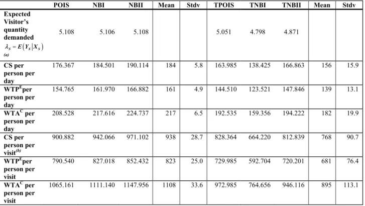
Both Marshallian and Hicksian welfare measures were estimated in this study. Table 4
reports CS, WTPE, and WTAC per person per visit, and per person per day. CS, WTPE, and WTAC per person per visit were calculated by the formulas (13) and (14), respectively. CS, WTPE, and WTAC per day were estimated by dividing the former measures byλS. Consumer Surplus per day of the representative visitor who took a trip
to the PGNP during the summer of 1994 for recreation purposes varies from 138 €
minimum in the TNBI distribution to 190 € maximum in the NBII distribution (37%).
The Consumer Surplus per each 5 days-length visit to the PGNP varies from 664 € in
the TNBI distribution to 971 € in the NBII distribution (46%). However, the differences
are not so sensitive within each group of distribution. The difference between the CS
per day calculated after the three generalised models is only 8% and within the
truncated models is 21%. The three welfare measures are hierarchically related as
theoretically expected for all the models, when we are dealing with welfare changes
varies from 124 € in the TNBI to 167 € in the NBII. Again the differences with the
WTPE are similar to those in CS. The welfare measures reveal some sensitiveness to the estimation procedures, particularly in the group of the truncated distributions, but not as
high as what we would expect, from the analysis of the empirical results of other
TCM’s studies. However, the differences are sufficiently important to estimate the
intervals of confidence for the welfare measures35. The same moderated sensitiveness is revealed between the welfare estimates and the time cost procedure (e.g. WTPE varies only 8% from the POIS lower level to the higher NBII level, while CS estimated from
NBII varies only 17% between the lower level (zero time cost) to the higher level (time
cost equal to 50% of the available recreation income). Aggregating the WTPE of the representative visitor per day calculated by the TNBI model across the sample following
equation (3) generates the sample’s WTPE, for one day of recreation in the PGNP, which is 30016 € (123 ). These values mean that the PGNP’s representative
visitor gets a use benefit of 124 € per each day in the park, and 593 € per each visit of 5
days. The recreation use value of 1215 days in the park is 150660 € (1215 ). 521 243×
.
124 euros ×
3. The TRV of the PGNP
The values estimated in section 2 are related with the recreation use benefits of a sample
of visitors, during the summer season. Nevertheless they may be interpreted as being
representative of annual instead of seasonal values, because of the seasonal
characteristics of outdoor recreation. Besides, the values reflect the recreation value at a
single present moment, but do not account for the temporal dimension of natural
recreation use values. But as the PGNP’s is a reproducible asset yielding annual
recreation benefit flows over several time horizons, in practice this means that if we
assume: i) the visitor preferences are fix; ii) the PGNP maintains there natural
characteristics and availability for recreation, then the 243 visitors of the sample will
annually beneficiate of a 150660 € benefit flow equivalent to 1215 days of use.
Therefore, to obtain the sample’s TRV of the PGNP over a period T (say 30, 50, 100 or
300 years and more) we will summing up the present recreation value of the
single-period welfare measure calculated in section 2, by using a discount rate, following the
35 Confidence intervals around these measures will be measured latter on, by using a re-sampling technique known as bootstrapping.
equation (4)36. Due to several reasons already explained in the paper, WTPE estimated by the TNBI model will be used to calculate TRV of the PGNP. Discounted
utilitarianism has proven particularly controversial when applied to environmental
valuations37. The origins of such controversy are: the practice of discounting itself; the number used to measure the discount rate ρ; and the irreversibility, risk, and uncertainty
surrounding futures outcomes (Freeman III 2003; Heal 1998). Albeit all the still
persisting controversy about discounting, Heal (1998, 1985) demonstrated that
discounting future utilities is in some sense logically necessary. A growing body of
empirical evidence suggests that the discount rate that people apply to future projects is
positive, not zero, and depends on the futurity of the projects and the magnitude of
income involved (Cropper et al 1994; Lowenstein and Elster 1992; Lowenstein and
Prelec 1992; Lowenstein and Thaler 1989; Thaler 1981). Because utilitarian geometrical
discounting based on a positive constant rate is discriminating against future generations
by attributing less weight to their utility levels while empirical evidence seems to deny
the constancy of the discount rate, some economists began to think over alternatives to
the classical utilitarian approach. Logarithmic discounting or hyperbolic discounting is
one such alternative38 (Lowenstein and Prelec 1992). Another problem with utilitarian discounting is about the number that shall be assigned to the rate of discount. Arrow et
al 1996 advocate that there are basically two approaches to choose the discount rate, the
prescriptive approach and the descriptive approach. Under the former, lower future
discount rates must be used (tending to zero) in contrast with the last approach that
relies fully on historical market rates of return to measure the discount rate. In practice,
policy makers have, in certain cases, applied lower discount rates to long-term
intergenerational projects (Bazerlon and Smetters 1999). More recently Weitzman 2001
demonstrated that the very wide spread of professional opinion on the discount
framework mean that declining discount rates should be used, around 4% annum for the
immediate future down to around zero for the far-distant future (300 years and more).
Another major issue in ecosystem evaluation has been how to account for the fact that
preserving an ecosystem is likely to represent an impediment to alternative economic
investment that might generate a higher rate of return than the effective interest rate
governing individual intertemporal substitutions. In doubt, and where the environment
36 The default criteria used by economists to include time is provided by the discounted utilitarianism framework which has thus far
dominated more for lack of convincing alternatives than because of the conviction it inspires.
37 For discussions see Nordhaus 1994, and Portney and Weyant 1999. 38
is involved, most non-economists and economists take the view that a lower rate is more
adequate when geometric discount is applied, as it attaches greater weight to the
interests of future generations than a higher one. Beyond the controversy surrounding
discounting framework and its arithmetic, some other questions arise when ecosystem
valuation is under discussion, such as irreversibility and uncertainty over visitor’s
preferences39. The former inflationates the ecosystem’s scarcity value (Krutilla and Fisher 1985). The later has large consequences for optimal choice and welfare measures
related with preference aggregations (Pizer 1998; Arrow et al 1996). Regardless, some
authors prefer to choose fix overtime preferences because of the difficulties with
preference aggregations (Nordhaus and Popp (1997) for instance). To compute (4) to
estimate total recreation use value of PGNP, we are going to follow the Weitzman
(2001) hyperbolic discounting framework for a period of time T equal to 50 years.
These mean that the Immediate Future (1-5 years) is discounted at 4% marginal rate; the
Near Future (6-25 years) at a 3% marginal rate; the Medium Future (26-50 years) at a
2% marginal rate; and finally the Distant Future (76-300 years) at a 1% marginal rate.
Therefore, by using (4) and the Weitzman (2001) hyperbolic discounting framework, if the PGNP will maintain their ecosystems holding the same natural characteristics and
amenities for 50 years, and if it will be available for recreation use, than one day of
recreation will generate a total recreation use value of 3874 €. The total recreation use
value for the representative visitor during 50 years, per visit, will be worth 17896 €, and
1215 recreation use days in the park worth 4369434 €. Due to difficulties with
inter-temporal preference aggregations, it is assumed that individual preferences are fixed and
equal to those at the present time. In practice this means that it will be assumed that the
present total recreation value as estimated in section 2 will be fix for the relevant period
of time T = 50.
4. Discussion and Conclusions
In this paper we calculate the willingness to pay by an average visitor of the PGNP
when he/she uses the park’s ecosystems as a natural capital to produce flows of outdoor
recreation services. Following the theoretical definitions of the recreation welfare
39 Visitors might be uncertain as to whether a specific ecosystem amenity flow will be available for their use in the future or whether
measures came the empirical application where a TCM’s individual version based on
count data models was used to estimate the PGNP’s recreation demand function and the
subsequent visitor’s Mashallian CS welfare measure, and the Hicksian CS and ES
welfare measures. These measures were estimated based on the hypothetical impact
assumption of a recreation price (cost) change for infinity of a day of stay in the PGNP
which in turn can be interpreted as PGNP closure or loss of access. To pass over some
problems related with the nature of the dependent variable and the way it is measured
and defined the following options were made. The dependent variable was defined as
the number of recreation days each visitor stayed in the park, during that visit, at the
moment of the questionnaire. By doing so it was possible to estimate the Marshallian
consumer surplus per each day, and per each visit, on average, for the representative
visitor of the sample, and the subsequent Hicksian welfare measure WTPE per day and per visit. Count data models were used to estimate the recreation demand function,
because the number of recreation days per trip are non-negative integers, and the sample
is truncated at zero. Therefore, the use of common regression linear methods with this
type of data sample would generate inefficient, biased, and inconsistent estimations. We
obtained the following results. One recreation day in the PGNP at the present moment
of the questionnaire values 124 € (2005 prices) for the average representative visitor of
the sample, and 593 € per each average five days length visit. Thereupon, we considered
that if the average representative visitor would keep on visiting the park for 50 more
years, the total recreation value of each day visit would be 3 874 € and each average
five days length visit would be worth 17 896 €. These are relatively large use values for
the users of the PGNP. To have a more precise idea about the values involved in the
year of the questionnaire, approximately 12 000 visitors camped in PGNP generating a
present recreation value per day of visit of 1 488 000 € (12 000 124 × euros)), and of 7
116 000 € (12 000 593 × euros)per each average five days length visit. To infer about
the population use value of PGNP some caution has to be taken. Though the parameter
estimators of the demand curve are consistent for the population, it does not guarantee
that the representative visitor based in the sample is representative for the population.
This is due to the fact that the explanatory variables observed, the visitors’
characteristics, come from the truncated distribution and following Santos Silva (2003)
the truncated distribution of the independent variables is different from the un-truncated
thought as representative of those that actually visited de park and not of the entirely
population. Therefore, only those measures that depend exclusively on the parameters
of the demand curve, as the Marshallian CS per day, can be used to make predictions for
the population. Consequently, if for example 1% of the 18th and more year old Portuguese population went to visit the PGNP, a 10 6
10 euros
× 40
( 70262 )
total present use benefit per day would be generated, while 25% of the same population
would generate a total present use benefit of
138 euros
×
6 10 euros
242× 41 per day. Applying the same ratiocination to half of the population, one recreation day in the PGNP would have
a present benefit value almost equivalent to half’s that of the Vasco da Gama’s bridge42. The results indicate that PGNP’s visitors receive a considerable amount of benefit from
the recreation use of PGNP’s ecosystems which allow us to conclude that the park has a
high hidden economic value and is a valuable asset for society. This suggests that
management resource should be allocated to recreation use, specifically to eco-tourism
activities, as a mean to develop the local area in a sustainable way, and in full respect of
the conservation goals which are priority. Besides, the large estimated use value would
suggest yet that undertaking major improvement work for the existing natural facilities
that would probably be economically and socially justifiable. For instance, one of the
problems with the PGNP is a certain degree of congestion during the peak-load summer
season, where many people share the PGNP while revealing behaviours that are not
compatible with nature conservation goals. The price/recreation cost elasticity suggests
that if the management entities of the park would want to implement entry or access
fees, that would not have any dramatic effect upon recreation days demand per trip.
Besides, during the questionnaire phase of this study, visitors were asked if they were
prepared to pay an access fee and 23% answered Yes. At a first glance, this percentage
does not seem particularly enthusiastic, but it is nevertheless important for the
Portuguese case and similar countries, where people are not used to the idea of paying
an access fee for the right of using nature. The major limitations of our study are the
small sample size and perhaps the lack of some socio-demographic variables. Also we
only estimate the point welfare measures but not the confidence intervals which will be
done later on. Another limitation is the lack of statistical information about the annual
number of visitors. If the PGNP’s managers would allocate resources to obtain this
40 This is 0.007% of the Portuguese GDP at market prices, 0.03% of the North Region’s GVA at basic prices, and 1% of the
agricultural GVE at basic prices of the same region.
41 This is 0.2% of the Portuguese GDP at market prices, 0.89% of the North Region’s GVA at basic prices, and 26% of the
agricultural GVE at basic prices of the same region.
424 8 5 and
8 9 7 , respectively.
6
1 0 eu ro s
× 6
statistical information, the conclusions of this study could be used to quantify the stock
recreation value of the PGNP.
Acknowledgements
We wish to thank João Caravana Santos Silva for their helpful comments and
suggestions. Any remaining errors are of course our own.
Appendix: the Estimators
The standard POIS model assumes that the non-negative integer nature of recreation demand data can be
described as the result of many discrete choices, satisfying a Poisson discreet probability distribution,
( ) ( ) exp( ) 0
Pr , ,
!
k i
ob Y k f k k
λ λ λ −
= = = ∀ >
i
Y
( )
exp
i Xi
where i = 1, 2, …, N visitors, Yi is the i
th
observation on the
number of days in the park per trip, and k = 0, 1, 2, … is the set of the possible nonnegative integer values
that can take. λ is the Poisson parameter. The model can be extended to a regression by setting
λ = β where Xi is the matrix of explanatory variables and β the Poisson parameters to be
estimated. The exponential specification is used to restrict λito be positive as is required for a proper distribution. The log-likelihood of the model is:
( )
1
ln exp ln !
n
i i i
i
L Xβ Y Xβ
=
=∑− + − Yi
The conditional mean of Yi is given by:
( i i) i exp( i )
E Y X =λ = X β
Conditional variance equals the conditional means. However if there is over dispersion, the first is
consistently estimated using standard POIS model but the standard errors of the estimators βare biased
downward (Grogger and Carson 1991). Cameron and Trivedi (1990) developed tests for over dispersion
in the POIS model.
In the presence of over dispersion the negative binomial estimator, a generalisation of the POIS model, is
a possible solution to this problem. The NB probability
( ) ( ) ( ) [ ] 1 1 1 1 1
Pr i NB( ) i k i k
k
ob Y k f k
k
α
α αλ αλ
α
− +
Γ +
= = = +
Γ + Γ
where α>0, and λi are distributed as gamma random variables Γ( ).. αis a nuisance parameter to be estimated along with β.
The conditional mean is:
( i i) i e xp( i )
E Y X = λ = X β
and the conditional variance is:
( i i) i(1 i)
Var Y X =λ +αλ
so that Var Y X( i i)>E Y X( i i). The ratio variance-mean 1+αλi is the degree of over dispersion. This
specification is known as Type II Binomial Model (NBII). The log-likelihood of the model is:
( )
(
)
( ) ( )1
1 1 1
1 1
ln ln ln ln ln log
n
i i
i
L k k k αλ k αλ
α α α
=
= Γ + − Γ + − Γ + − + +
∑
If there is truncation at zero, which occurs when zero visits demand is not observed by the visitor
sampling, the truncated POIS (TPOIS) and NBII (TNBII) can be used.