Comparative analysis of the results from two different frequency grouping methods on the currents and temperatures of an induction motor submitted to harmonics and interharmonics : laboratory tests

i

Comparative Analysis of the Results from two

Different Frequency Grouping Methods on the

Currents and Temperatures of an Induction

Motor Submitted to Harmonics and

Interharmonics - Laboratory Tests

CHRISTIAN CHUKWUEMEKA ABADA

DISERTAÇÃO DE MESTRADO

PROGRAMA DE PÓS-GRADUAÇÃO EM ENGENHARIA ELÉTRICA DEPARTAMENTO DE ENGENHARIA ELÉTRICA

FACULDADE DE TECNOLOGIA

UNIVERSIDADE DE BRASÍLIA

iii

CATALOG

ABADA, CHRISTIAN CHUKWUEMEKA

Comparative Analysis of the Results from two Different Frequency Grouping Methods on the Currents and Temperatures of an Induction Motor Submitted to Harmonics and Interharmonics - Laboratory Tests [Distrito Federal] 2018.

xiii, 78 p., 210 x 297 mm (ENE/FT/UnB, Mestre, Dissertação de Mestrado - Universidade de Brasília, Faculdade de Tecnologia.)

Departamento de Engenharia Elétrica

1. Frequency Grouping Method 2. Three-phase Induction Motor

3. Harmonics and Interharmonics 4. Electric Current and Temperature Analysis I. ENE/FT/UnB II. Title (série)

BIBLIOGRAPHICAL REFERENCE

ABADA, C. C. (2018). “Comparative Analysis of the Results from two Different Frequency Grouping Methods on the Currents and Temperatures of an Induction Motor Submitted to Harmonics and Interharmonics - Laboratory Tests”, Master Dissertation, PPGENE.DM-704/2018, Department of Electrical Engineering, Faculty of Technology, University of Brasilia, Brasilia/DF, 79 p.

ASSIGNMENT OF RIGHTS

AUTHOR: Christian Chukwuemeka Abada

TITLE: Comparative Analysis of the Results from two Different Frequency Grouping Methods on the Currents and Temperatures of an Induction Motor Submitted to Harmonics and Interharmonics - Laboratory Tests.

DEGREE: Master YEAR: 2018

The University of Brasília is granted permission to reproduce copies of this master's dissertation and to lend or sell such copies only for academic and scientific purposes. The author reserves other publishing rights and no part of this master's dissertation may be reproduced without the written permission of the author.

____________________________ Christian Chukwuemeka Abada

SQN, 406 Bloco L, APT. 203, Asa Norte. christian.abada.ch@gmail.com

iv

PREFACE

I dedicate this work to GOD, for His infinite grace and favor in my daily life.

To my family, for their endless love, support and prayers.

To the union church family, for all their wonderful words of encouragement and prayers.

To my son, Uchechukwu, for coming into my life in a time of difficulties and giving I more reason to smile and follow my dreams.

To my supervisor, Prof. Anésio de Leles Ferreira Filho, I am sincerely grateful for your patience, valuable orientations, and the long hours of discussions from which I could always learn.

To my post-graduate colleagues, Marcos Diego Castro e Silva and Guilherme Zanetti Rosa for your dedication and contribution during the entire process of this research.

To Luiz Valadão, for the long hours of discussions and important contributions that helped me understand the procedures necessary toward archiving the main objective of this study.

To all members of the Laboratory of Intelligent Network of the University of Brasília, for your contribution and friendship during my research period.

To the University of Brasília and professors of the Programa de Pós-Graduação de Engenharia Elétrica da UnB, for the opportunity and invaluable contribution towards learning.

To the Coordenação de Aperfeiçoamento de Pessoal de Nível Superior (CAPES), for the financial assistance through the scholarship granted.

v

ABSTRACT

Comparative Analysis of the Results from two Different Frequency Grouping Methods on the Currents and Temperatures of an Induction Motor Submitted to Harmonics and Interharmonics - Laboratory Tests

Author: Christian Chukwuemeka Abada Supervisor: Anésio de Leles Ferreira Filho

Programa de Pós-graduação em Engenharia Elétrica Brasília, July 2018

The continue advances in power electronics have resulted in the installation of non-linear power loads such as motor drive systems and power converters which can lead to disturbances like the harmonics and interharmonics. Despite the significant growth of the application of inverters in renewable sources such as wind and photovoltaic (PV), the analysis of interharmonics in power systems is still, characterized as a challenge. In fact, the measurement of harmonics have been broadly discussed and investigated in the literature. However, on the issue of interharmonics, one can observe the lack of studies aimed at investigating the grouping of interharmonics and their effects on equipment of the electric power system such as the three-phase induction motor (TIM). In order to be able to associate harmonic and interharmonic components with their effects on the TIM, it is necessary to adopt the frequency grouping method.

In view of this, the IEC 61000-4-7 international standard suggests the concept of grouping for measuring interharmonics. The approach refers to the calculation used to group various values of a parameter in a single representative value at specific time intervals. This method has been employed in some studies in the literature regarding this topic. Nevertheless, it has been reported in written matter that the resulting group harmonics and/or interharmonic group lose some characteristics of the usual harmonic or interharmonic frequency component. This problem instigated a study in the literature that proposed the idea of group frequency (GF). The GF represents a single frequency component of a current or voltage signal placed on a given band so that the individual components have the same power index as that of all the frequency components in the band.

vi The present study compares the results from the aforementioned grouping methods with the aim of identifying, which, based on laboratory tests, best represents the influence of harmonics and interharmonics on the currents and temperatures of the TIM. The use of a precise grouping method constitutes an important step in studies aimed at identifying the effects of interharmonics on equipment such as the TIM.

Keywords: Frequency grouping methods, Three-phase induction motor, Harmonics and Interharmonics, Currents and Temperatures.

vii

TABLE OF CONTENTS

PREFACE...iv

LIST OF TABLES………..ix

LIST OF FIGURES……….x

LIST OF SYMBOLS AND NOMENCLATURES……...………...…….xi

1 – INTRODUCTION...1

1.1 – INITIAL CONSIDERATIONS...1

1.2 – OBJECTIVES OF THE DISSERTATION ...2

1.3 – LITERATURE REVIEW.………..………...3

1.4 – CONTRIBUTIONS OF THE DISSERTATION...7

1.5 – DISSERTATION LAYOUT...7

2 – THEORETICAL FOUNDATION………...8

2.1 – INITIAL CONSIDERATIONS...8

2.2 – CAUSES AND EFFECTS OF HARMONIC AND INTERHARMONIC DISTORTIONS………...………...8

2.3 – SPECTRAL ESTIMATION METHOD………...………...10

2.4 – THE IEC GROUPING METHOD………...………...11

2.5 – THE CHANG GROUPING METHOD………...14

2.6 – ALGORITHMS FOR SIMULATING THE GROUPING METHODS…………..21

2.7 – FINAL CONSIDERATIONS………..25

3 – EXPERIMENTAL APARATUS AND METHODOLOGY………....….26

3.1 - INITIAL CONSIDERATIONS...26

3.2 - EXPERIMENTAL APARATUS...26

3.3 – DATA BANKS………..……….29

3.3.1 – Definition of the Data Bank……….………..…...29

3.3.4 – Data Bank 1 (DB1)………..……..………....31

viii

3.5 – PROCEDURES FOR COMPARING THE GROUPING METHODS…………...33

3.6 – FINAL CONSIDERATIONS………..34

4 – RESULTS AND ANALYSIS………...35

4.1 – INITIAL CONSIDERATIONS……..……….35

4.2 – ORIGINAL FREQUENCIES AND THEIR CORRESPONDING GROUP FREQUENCIES……….………….…35

4.3 – COMPARATIVE ANALYSIS OF THE ELECTRIC CURRENTS FROM THE GROUPING METHODS………37

4.4 – COMPARATIVE ANALYSIS OF THE TEMPERATURES FROM THE GROUPING METHODS………42

4.5 – FINAL CONSIDERATIONS……….…….47

5 – CONCLUSIONS AND SUGGESTIONS……….………...48

5.1 – CONCLUSIONS………...……..48

5.2 – SUGGESTIONS……….………50

BIBLIOGRAPHY………..51

ix

LIST OF TABLES

Table 3.1 - Data Bank 1: Interharmonic frequencies and harmonic orders applied to the TIM………..31 Table 3.2 - Number of conditions applied to the TIM and the duration of each of the data bank………...………...33 Table 4.1 - Differences between the currents of the Original, Chang and IEC signals………..………40 Table 4.2 - Differences between the temperatures of the Original, Chang and IEC

x

LIST OF FIGURES

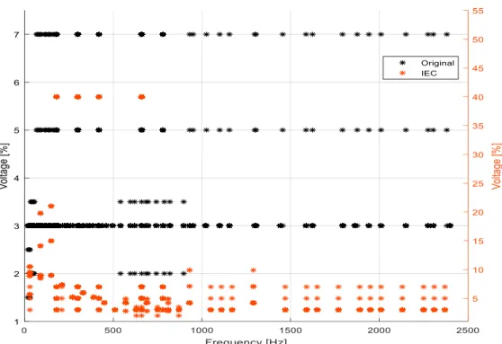
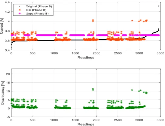
Figure 2.1 - Illustration of the principle of the interharmonics groups. Source: Hanzelka and Bien, (2004)………..………..…...………12 Figure 2.2 - Spectrum grouping according to IEC………...………14 Figure 2.3 - Pictorial of the concept of a group frequency. Source: Chang et al., (2004)………...16 Figure 2.4 - Phasor diagram of interharmonic components. Source: Chang et al., (2004)………...18 Figure 2.5 - Sequence predominance in a system operating at 60 Hz. Source: Chang et al., (2004)………...………..19 Figure 2.6 - Sequence dominant frequency bands for a 60 Hz power system. Source: Chang et al., (2004)………..………20 Figure 2.7 - Algorithm for the IEC grouping………23 Figure 2.8 - Algorithm for the Chang grouping………..………….24 Figure 3.1 - Scheme of the control system and quantities report generation. Source: Silva M.D. et al., (2018)………27 Figure 4.1 – Original frequencies and voltage amplitudes with their correspondents from the IEC grouping method……….36 Figure 4.2 - Original frequencies and voltage amplitudes with their correspondents from the Chang grouping method………...…..36 Figure 4.3 - Currents and discrepancies of the original signal and IEC grouping method……….…38 Figure 4.4 - Currents and discrepancies of the original signal and Chang grouping

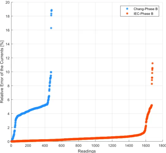
method……….38 Figure 4.5 - Relative error of the electric currents resulting from the Chang and IEC

grouping methods………41 Figure 4.6 - Temperatures and discrepancies of the original signal and IEC grouping

method………...…..42 Figure 4.7 - Temperatures and discrepancies of the original signal and Chang grouping

method……….………43 Figure 4.8 - Relative error of the temperatures resulting from the Chang and IEC grouping

methods………46 Figure A.1 - Currents and discrepancies of the original signal and IEC grouping method from phase A………57

xi Figure A.2 - Currents and discrepancies of the original signal and IEC grouping method from phase C………58 Figure A.3 - Currents and discrepancies of the original signal and Chang grouping method from phase A………...58 Figure A.4 - Currents and discrepancies of the original signal and Chang grouping method from phase C………...……….59 Figure A.5 - Relative error of the electric currents resulting from the Chang and IEC grouping methods (Phase A)………..………..60 Figure A.6 - Relative error of the electric currents resulting from the Chang and IEC grouping methods (Phase C)……….61 Figure A.7 - Temperatures and discrepancies of the original signal and IEC grouping method from phase A………...62 Figure A.8 - Temperatures and discrepancies of the original signal and IEC grouping method from phase C………....63 Figure A.9 - Temperatures and discrepancies of the original signal and Chang grouping method from phase A………...63 Figure A.10 - Temperatures and discrepancies of the original signal and Chang grouping method from phase C………...64 Figure A.11 - Relative error of the temperatures resulting from the Chang and IEC grouping methods (Phase A)………..………..65 Figure A.12 - Relative error of the temperatures resulting from the Chang and IEC grouping methods (Phase C)……….66

xii

LIST OF SYMBOLS AND NOMENCLATURES

Nomenclatures

AC

Alternating Current;

°C

Degree Celsius – unit of temperature;

CIGRÉ

Conseil International des Grands Réseaux Életriques;

DC

Direct Current;

DFT

Discrete Fourier Transform;

FFT

Fast Fourier Transform;

GF

Group Frequency;

IEC

International Electrotechnical Commission;

IEEE

Institute of Electrical and Electronics Engineers;

THD

Total Harmonic Distortion;

TIM

Three Phase Induction Motor;

PV

Photovoltaic;

Symbols

𝐺

Magnitude of the interharmonic group;

𝐶

Magnitude of each interharmonic component;

𝑛

Harmonic order;

𝑓

Frequency representing the interharmonic group;

f

Fundamental frequency of the system;

ℎ

Frequency component of the n

_-order;

𝑁

Spectral control window;

𝑉

Amplitude of the Fourier component;

K

Power quality index;

xiii

𝑓

Lower border frequency;

𝑓

Upper border frequency;

k

Scanning counter of the original frequency spectrum;

kk

Counter of the frequencies obtained in the grouping process;

floor

Command that allows the rounding of any number to its own

integer;

I

Electric Current Circulating through phase A of the stator

winding;

I

Electric Current Circulating through phase B of the stator

winding;

I

Electric Current Circulating through phase C of the stator

winding;

T

Temperature of the stator winding in Phase A (°C);

T

Temperature of the stator winding in Phase B (°C);

T

Temperature of the stator winding in Phase C (°C).

1

1 - INTRODUCTION

1.1 - INITIAL CONSIDERATIONS

In industries where many applications require a precise speed control and monitoring of the driving equipment, the use of the three-phase induction motor (TIM) has driven the development of electronic speed controllers based on the switching of semiconductor devices. These aspects have therefore instigated the development of studies related to the effects of using frequency inverters on the TIM. Concerning this matter, the preponderance of two specific approaches is noted in the literature: the analysis of the influence of the parameters of the inverter operation on the performance of the machine; and the investigation of the disturbances caused at the input of the inverter (Oliveira, 2013). Among these disturbances, the issue of interharmonics, which has been considered more damaging than integer harmonics components of the distorted signals, can be highlighted. (Hao et al., 2007).

In addition to the typical effects caused by harmonics, such as overheating and reduction in lifetime, interharmonics create, even at low amplitudes, some new problems, such as sub synchronous oscillations, voltage fluctuations and, consequently, flicker. The presence of interharmonic components has also introduced new and important effects in terms of variations in waveform (Feola et al., 2012). These phenomena are observed in an increasing number of loads and consequently making the investigations related to the subject more relevant. (Testa et al., 2007).

In consideration to the aforementioned reason, the effects of interharmonics on the power system have been broadly discussed in the literature (IEEE Interharmonic Task Force, 1997, Hao et al., 2007, Testa et al., 2007, Feola et al., 2012, Arrillaga, J. and N.R. Watson, 2003, Chang et al., 2004, Li et al., 2003, Macedo Jr, J. R., 2009, Hanzelka, Z. and Bien, A., 2002, Hui et al., 2012, H.C Lin, 2014, Marz, 2014). Moreover, this phenomenon has proven to be a relevant area of investigation for studies involving their effect on some power quality parameter of the electric system.

2 However, it is possible to identify lacunas in investigations regarding the effects of interharmonic distortions and the grouping of interharmonic components. It is noteworthy that in order to study the effects of interharmonics, the use of interharmonic group is necessary because the analysis based on the separate usage of only one interharmonic order is not enough.

It should be heightened therefore that, this topic is characterized today as important and relevant since the increasing use of inverters in wind and photovoltaic sources in the electric system is no longer seen as a trend, but as a reality in various parts of the world.

1.2 - OBJECTIVES OF THE DISSERTATION

The main objective of this study is to analyze the spectral component grouping methods and identify which, based on laboratory tests best represent the effects of harmonics and interharmonics on the currents and temperatures of a TIM. These quantities have been observed in the literature to be influenced by interharmonics, mainly for situations in which the interharmonic frequency components are greater than that of the power system.

In order to reach the main goal of this dissertation, it is necessary to meet the following specific objectives:

 To carry out an investigation in the literature related to the issue of the characterization of the effects of harmonic and interharmonic distortions in electric machines, observing the already studied line of research and the concepts necessary for developing this theme.

 To select the data bank that will be used in laboratory tests to generate signals containing harmonic and interharmonic distortions, with the capacity of permitting the identification of the advantages and disadvantages of the grouping methods under evaluation;

3 as well as the subjection of the TIM to these reconstituted signals;

 To identify the grouping method that best represents the effects of these signals containing harmonic and interharmonic distortions on the currents and temperatures of the TIM.

1.3 - LITERATURE REVIEW

The investigations carried out worldwide in the electric sector on issues related to power quality have been expressive, providing relevant results for the control of energy efficiency as well as solving problems that are characterized as critical for this scenario.

One of the issues highlighted by experts in the field is the need for research on the influence of interharmonics in the electric sector, particularly the effects on electric machines.

In (IEEE Interharmonic Task Force, Cigré 6.05/CIRED and 1000-2-1, C.I., 1990) it was highlighted that between the harmonics of the power frequency voltage and current, further frequencies that are not integers (multiple) of the fundamental can be observed. They can appear as discrete frequencies or as a wide band spectrum.

According to (Arrillaga, J. and N.R. Watson, 2003), power system harmonics are defined as sinusoidal voltage and currents at frequencies that are integer multiples of the main generated (or fundamental) frequency. They constitute the major distorting components of the main voltage and load current waveforms. However, the increasing content of power system interharmonics, i.e. distorting components at frequencies that are not integer multiples of the fundamental, has prompted a need to give them greater attention.

Studies on harmonics and interharmonics and their effects on the power system have being becoming of great importance. In (Li et al., 2003), the authors mentioned that large number of studies related to the subjects of interharmonics sources, impacts, measurements, limit values and mitigations has been published. Nevertheless, the difficulties in finding accurate interharmonic frequency and magnitude still leave this

4 field of studies with many questions.

In (Chang et al., 2004), interharmonics were said to be able to degrade the performance of a power system and the impacts were considered to be: potential shaft damage in drive motors; heating effect due to loss; voltage distortion owing to voltage drop in the network impedance and loss of life of filters. Therefore, to understand and reduce the impact of interharmonics, a proper analysis is needed.

In (Macedo Jr, J. R., 2009), it is noted that the low-frequency oscillations in mechanical systems are originated fundamentally by the property of the interharmonic components frequencies in causing a modulation in the effective (or peak) values of the voltages and electric currents that feed such systems. Some interharmonic components, notably subharmonic, can stimulate mechanical oscillations in rotating machine systems due to the potential excitation of mechanical resonances, thus reducing the lifetime of the machines.

Furthermore, it was observed in (Macedo Jr, J. R., 2009), that additional heating in the stator winding of an induction motor coupled with the presence of 0.1% subharmonic voltage component at the motor terminals is equivalent to the additional heating caused by 1.0% of voltage unbalance present at the same terminals.

In (Hanzelka, Z. and Bien, A., 2002), it was pointed out that induction motors can be interharmonic sources because of the slots in the stator and rotor iron, particularly in combination with the saturation of the magnetic circuit (called "harmonic slots"). At rated motor speed, the frequencies of the components that cause disturbances are usually in the range of 500 Hz to 2000 Hz, but they can expand significantly during the starting period. The authors mentioned that natural engine asymmetries (rotor misalignment, etc.) could also be sources of interharmonics.

In (Testa et al., 2007), it is noted that the presence of interharmonic components strongly increases difficulties in modeling and measuring the distorted waveforms. This is mainly due to 1) the very low values of interests of interharmonics (about one order of quantity less than for harmonics), 2) the variability of their frequencies and amplitudes, 3) the variability of the waveform periodicity, and 4) the great sensitivity to the spectral leakage phenomenon.

5 Interharmonic currents cause interharmonic voltage distortions that depend on the intensities of the current components and the impedance of the power supply system at that frequency. The higher the frequency ranges of the current components, the greater the risk of a resonance phenomenon, which can increase voltage distortion and cause overloads or disturbances in the operation of customer equipment and installations (Hanzelka, Z. and Bien, A., 2002).

The methods for eliminating the effects of interharmonics, according to (Hanzelka, Z. and Bien, A., 2002), include reducing the level of emission; reducing the sensitivity of loads and improving the coupling between generators and loads. Moreover, the authors also stated that there are no coherent regulations and norms concerning interharmonics, despite the fact that there is a great practical need for them.

In (Hui et al., 2012) it was discussed that some interharmonics frequency components are very close to a harmonic frequency and therefore can cause severe waveform modulation. The authors proposed a signal processing method that can separate interhamonic and harmonic components in close proximity. The proposed method is based on the estimation of leakage values caused by interhamonics at harmonic frequencies.

According to the recommendations in the international standard IEC 61000-4-7, voltage interharmonics are limited to 0.2% for the frequency range from the DC component to 2 kHz. However, in (Testa et al., 2007), the authors emphasizes that this low limit value aims to ensure compliance with interharmonic voltage distortion with illumination systems, induction motors, thyristor devices and remote control systems. Due to the measurement difficulty, they presented some alternatives, namely: to limit the interharmonic voltage distortion, the individual component must be less than 1%, 3%, or 5% (depending on the voltage level) for range 0 to 3 kHz; adopt limits correlated to the short-term value in case of a serious level of flicker, that is, equal to 1.0; and develop appropriate limits for equipment and system effects, such as mechanical generator systems, signaling and communication systems, filters, etc.

The key to the measurement of both harmonics and interharmonics in the IEC 61000-4-7 standard is the utilization of a 10-cycle sample window for 50 Hz systems or a 12-cycle

6 sample window for 60 Hz systems. The IEC grouping method is a practical tool for measuring interharmonics because it can reduce the effects of spectrum leakage, as well as disclosing the interharmonic levels. However, the spectrum resolution with 5 Hz is not sufficiently precise to reflect the practical interharmonic locations for both 50 Hz and 60 Hz systems (Lin et al., 2011 and H.C Lin, 2014).

The IEC 61000-4-7 standard introduced the concept of group-interharmonics as a suggestion toward the measurement of the interharmonic components. These harmonic and interharmonic components, according to the standard, can be grouped into harmonic groups, interharmonic groups, harmonic subgroups and interharmonic subgroups.

A new grouping method based on the limitation of the frequency group by the predominance of the symmetrical components and the weighting of the group frequency by the amplitude of the individual components was presented in (Chang et al., 2004). In this study, the authors performed a simulation in which the waveform is switched and load is linear, therefore resulting in interharmonic components when the current spectrum is obtained. It was concluded that the concept of group frequency could be used to facilitate the analysis of interharmonics in power systems frequencies and when compared with the new IEC standard, group frequencies is found to better maintain the characteristics of the frequency components after grouping.

In (Aiello et al., 2006), experiments and measurements were carried out in a small photovoltaic installation in order to compare some possible ways of calculating THD when applying the IEC 61000-4-7 groupings. From the study, it is clear that the use of subgroups is very useful for the signals originating from a photovoltaic inverter.

It is therefore observed that although interharmonics are of great concern in the electric sector, there is still a lack in literature, of studies that deeply present the effects of these phenomena on the network and the importance of using interharmonic groupings in measuring and modeling interharmonics.

7 1.4 - CONTRIBUTIONS OF THE DISSERTATION

The major contribution of this study is to identify the best grouping method for interharmonics among those evaluated in this study. However, another contribution of this study is the exhibition of the results of the grouping methods on the currents and temperatures of the application of harmonics and interharmonics on a TIM.

1.5 - DISSERTATION LAYOUT

In order to meet the objectives and contribution of this dissertation, the layout of the dissertation is described as follows.

Chapter 2 provides the theoretical foundation of this study. The causes and effects of harmonic and interharmonic distortions are deliberated. Next, some spectral estimation methods including the Chang and IEC grouping methods are discussed. Finally, the algorithms used for simulating the grouping methods are presented.

Chapter 3 is dedicated to the infrastructure and methodology used to reach the objectives of this dissertation. The experimental apparatus and the data banks containing the harmonic and interharmonic conditions in which the TIM will be subjected to are presented. Finally, a description of the procedure used for analyzing the grouping methods under study is presented.

In Chapter 4, the results obtained from this study are presented and discussed. They include the comparative analysis between the grouping methods under study and the determination of the most reliable grouping method in relation to the real waveform.

Chapter 5 presents a brief summary of what was carried out in this study and some concluding remarks about the study, including possible future work and projects that can be produced because of this study.

8

2 - THEORETICAL FOUNDATION

2.1 - INITIAL CONSIDERATIONS

This chapter is focused initially on describing the causes and effects of harmonics and interharmonics distortions on the power system. Then, the spectral estimation method related to the DFT as well as the IEC and Chang grouping methods are discussed. Finally, the algorithms for simulating the grouping methods are presented.

2.2 - CAUSES AND EFFECTS OF HARMONIC AND INTERHARMONIC DISTORTIONS

Harmonics and interharmonics are caused by the operation of non-linear loads (Testa et. al., 2007). These non-linear loads are set of devices and electrical elements in which the relationship between the voltage and current values do not obey Ohm's law. For the case of interharmonics, the main mechanism of generation is the operation of non-linear equipment that connect two AC systems of different frequencies, such as the frequency inverters (Hanzelka & Bierí, 2004).

Prior to the appearance of power semiconductors, the main sources of waveform distortion were electric arc furnaces, the accumulated effect of fluorescent lamps, and to a lesser extent electrical machines and transformers. The increasing use of power electronic devices for the control of power apparatus and systems has been the reason for the greater concern about waveform distortion in recent times (Arrillaga and Watson, 2003).

Regarding the effects on power systems, there are many studies on this topic for harmonic components. Concisely, the following effects can be attributed to the presence of these components: interference in communication systems; malfunction of electronic equipment and protective devices; losses in power generation; mechanical oscillations and deterioration of the lifetime of electric machines (Singh, 2007; Lee, 1998).

9 The issue of interharmonics is an advanced subject in the field of power quality, which lacks more consolidated methodological treatments in terms of measurement. In addition to being predecessors of similar impacts of harmonics, some authors point out that these components may culminate in specific effects, such as saturation of current transformers and the phenomenon of light scintillation (Hanzelka and Bierí, 2004, Testa et al. 2007). The latter, known as flicker, occurs due to voltage fluctuation, which in turn is linked to the presence of low-frequency interharmonics (Macedo, 2009).

Interharmonics characteristic are usually smaller than that of the harmonics and this is why less attention has been devoted to them compared to harmonics issue. However, with the rapid growth of electronic power applications, and consequently increasing the interharmonics distortion in the grid, special concerns have been raised to define limitations for interharmonics in respect to their frequencies and amplitudes (Soltani et. al., 2016).

Interharmonics near fundamental or harmonics could cause light flicker. However, these components are not easily detected due to leakage or resolution limit (C. Li et al., 2003).

Non-stationary signal is a major source producing non-integral bins, but they are not real interharmonics. They are attributed to the violation of basic Discrete Fourier Transform (DFT) assumption: stationary and periodical (C. Li et al., 2003).

Today, the fast growing installation of grid-connected Photovoltaic (PV) and wind systems has reinforced concerns on power quality (Oliva and Balda, 2003, Katiraei, Mauch and Dignard-Bailey, 2007 and Fuchs and Masoum, 2008). PV inverters might be one contributor of harmonics and/or interharmonics that are delivered to the grid, challenging the power quality of the utility networks (Varma et. al., 2016, Gallo et. al., 2013 and Enslin and Heskes, 2004, Infield et. al., 2004, Yang, Zhou and Blaabjerg, 2016 and Messo et. al., 2014).

In addition, studies in the literature have revealed that large-scale adoption of grid-connected PV inverters may be one contributor to the increasing interharmonics appearing in the grid currents, causing voltage fluctuations and light flicker (Koponen,

10 Hansen and Bollen, 2015, Aiello et. al., 2006, Chicco, Schlabbach and Spertino, 2009, Langella et. al., 2016, Testa et. al., 2016, Xu et. al., 2016 and Pakonen et. al., 2016).

With the constant increase in the penetration level of the PV systems, the impacts of interharmonics may become higher and worsen the power quality (Sangwongwanich et. al., 2017).

In light of the above issues, the need for the definition of limits and measurement of interharmonics becomes indispensable. In order to carry out such measurements, the International Electrotechnical Commission (IEC) created two standards applicable to the measurement of harmonics and interharmonics: IEC 61000-4-30 and IEC 61000-4-7. These documents form the basis of some of the major national and international protocols for measuring distortions.

One of the procedures for measuring interharmonics is that of the grouping method. The grouping methods refer to the calculations used to group various values of a parameter in a single representative value at specific time intervals. Although this method have proven to be very useful, specialists in the field have criticized the proposed grouping method and, studies like Chang et. al., 2004 have been carried out to improve it. These grouping methods will be discussed in the ensuing session of this dissertation.

2.3 - SPECTRAL ESTIMATION METHOD

Spectral estimation methods permit an easier perception and manipulation in the frequency domain of physical phenomena, by discretizing a sinusoidal signal in a time domain distorted signal (Lathi, 1998). The Discrete Fourier Transform (DFT) is one of the most commonly used methods in the technical literature for analyzing current and voltage harmonic signals. Its efficient computational application, with the Fast Fourier Transform (FFT) algorithm, contributes to its dissemination in several applications (Lathi,

1998).

The spectral estimation using the DFT produces accurate results when the signal analysed is stationary and the sampling is performed synchronously with the fundamental

11 frequency. However, the DFT calculation has its accuracy significantly reduced when synchronization is not ensured along with the signal truncation in the time-domain, that is, when the chosen DFT time-window length is not an integer multiple of the fundamental signal period. In time-varying conditions or even with stationary interharmonics, typical of environments with renewable sources, spurious spectral components that lead to misleading measurements of harmonic distortions will inexorably arise (Li, Xu & Tayjasanant, 2003; Testa et. al., 2007; Morrison et. al., 2009; Ribeiro & Duque, 2009; Jain & Singh, 2011; Hernandez, Ortega & Medina, 2014).

Due to the importance and need to investigate the effects of interharmonics in power systems, the grouping has been well studied, since it seeks to solve the problems caused by the lack of synchronism in the DFT process. In addition, it can provide a methodology for the definition of a merit figure that allows the association of the effects to a certain value.

2.4 - THE IEC GROUPING METHOD

According to the international standard IEC 61000-4-7, interharmonics generally do not vary only the magnitude, but also the frequency. In the attempt to develop a method to simplify the measurement process of interharmonics, the IEC suggested a method for measuring interharmonics based on the concept of grouping.

A group of interharmonics constitutes the grouping of the spectral components in the interval between two consecutive harmonic components. This grouping provides a global value for the interharmonic components that includes the effects of harmonic component fluctuations (IEC 61000-4-7, 2002). Figure 2.1 illustrates the principle of the interharmonics groups.

12 Figure 2.1 - Illustration of the principle of the interharmonics groups. Source: Hanzelka

and Bien (2004).

From Figure 2.1 it can be observed that the idea of this method is to group the frequency components between two adjacent integer harmonics. The resulting group harmonics lose some characteristics of usual harmonic frequency components like the power quality indices (Chang et al., 2004).

The IEC recommends the application of the DFT with a time window of 200 ms (12 cycles of 60 Hz). The analysis through the Fourier transform assumes that the signal is stationary. However, the magnitude of the electric system voltage can vary in time, spreading the harmonic components energy at adjacent interharmonic frequencies (spectral leakage).

To improve the accuracy of the voltage evaluation, the components produced by a 12-cycle window are grouped according to equation (2.1) for a system operating at 60 Hz (IEC 61000-4-7, 2002). The proposed 5 Hz frequency resolution results in increase in the values of the least-squared error because of the spectral leakage and the picket-fence effects. The leakage arises due to truncation of the time-domain waveform such that a fraction of a period existed in the analyzed waveform (G.W. Chang et al., 2008).

13 In addition to this problem, the 5 Hz resolution and group harmonic or interharmonic concept recommended by the IEC and IEEE might not be sufficient for interharmonic detection. Especially for those interharmonics that cause flickers (C. Li et al., 2003).

𝐺

= ∑ 𝐶

𝐺_𝑖ℎ is the magnitude of the interharmonic group;

𝐶𝑘+𝑖 is the magnitude of each interharmonic component.

In order to reduce the error, the components immediately adjacent to the harmonic frequencies are counted at this frequency, therefore reducing the fluctuation effects of the harmonic amplitudes (IEC 61000-4-7, 2002). Thus, the equation for calculating the group magnitude in a system operating at 60 Hz is then carried out as shown in equation (2.2).

𝐺

= ∑ 𝐶

9

𝑖=1

The frequency representing the group is established as the average frequency between two consecutive harmonic components, according to equation (2.3).

𝑓

=

𝑓

+ 𝑓

2

Where:

𝑛 corresponds to the harmonic order.

The standard specifies the DFT as a tool for obtaining the spectrum, not excluding the application of other principles of analysis, such as the filter bank or wavelet analysis,

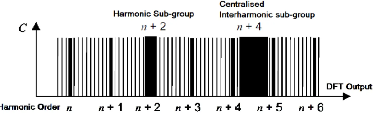
14 Figure 2.2 shows a grouping example that appears in the standard in question (IEC 61000-4-7, 2002).

Figure 2.2 - Spectrum grouping according to IEC.

From Figure 2.2, the main grouping forms performed by the IEC standard can be observed. In the case of the harmonic group of order 𝑛 + 2, the grouping of harmonic with adjacent interharmonics is noticed. For the interharmonic subgroup of order 𝑛 + 4, the grouping determination of the interharmonic components that are not adjacent between the harmonics 𝑛 + 4 and 𝑛 + 5 is observed.

2.5 - THE CHANG GROUPING METHOD

According to the authors, the grouping method presented in their study (Chang et al., 2004) allows an improvement of the spectral grouping method proposed by the IEC.

A long sampling window can be used in the DFT to analyze interharmonics. The longer the sampling window, the more frequency components can be analyzed. In the case where there are large number of frequency components, a long sampling window is required, therefore resulting in a long list of frequency components. The listing of all the analyzed frequency components is often inconvenient and ineffective (Chang et al., 2004).

The IEC proposes the method described above as a solution to this problem. However, this type of grouping results in the loss of some important physical aspects that are caused

15 by the frequency components in a system, such as the predominance of a symmetric component and the intensity of a given frequency in a particular band.

The Chang method proposed the concept of group frequency (GF) to facilitate the analysis of power system interharmonics as well as the conventional integer harmonics. A group frequency can be generalized for the analysis of load currents or voltages of other power devices (Chang et al., 2004).

A group frequency is defined as a single frequency component of a current or voltage signal placed on a given band so that the individual components have the same power quality index, e.g., the 𝐾-factor (the measurement of the ability of a transformer to serve non-sinusoidal loads), as that of all frequency components in the band (Chang et al., 2004).

One of the advantages of the GF is that a large number of frequency components of a load voltage or current are simplified to a few frequency components without significantly changing the power quality impact of the load current or voltage. The group frequency is said to keep more characteristics of the frequency components after grouping when compared to the IEC standard (Chang et al., 2004). Figure 2.3 shows the concept of a group frequency.

16 Figure 2.3 - Pictorial of the concept of a group frequency. Source: Chang et al., (2004).

In order to compute the group frequency, it is important to choose a frequency band for a GF and determine the power quality index that needs to be used.

To select the frequency band of each GF, the concept of the sequence dominant frequency band is used. In a balanced three phase power system, the fundamental component is

17 usually entirely of the positive sequence. When a non-linear, time invariant load is present, the load currents in the phases will be distorted and the distortion in phase B will occur [1

3] ∗ [ 1

𝑓0] seconds after it appears in phase A. Thus, if a second harmonic component

exists for the load current in phase B, it will occur two times delayed with respect to phase A, that is, in 120° and -120° in phase C. Thus, the second harmonic component is in negative sequence (Chang et al., 2004).

Analogously, the third harmonic component will only have zero sequence. With this, the sequences of higher integer harmonic components fall into the familiar pattern +, −, 0, +, −, 0, … (Chang et al., 2004).

Where f0 is the power frequency.

The same logic can be used to observe the predominance of symmetrical components in relation to interharmonics. Figure 2.4 shows the behavior of phasors for interharmonic components. In which, the first row shows the zero sequence dominant frequency components (e.g., 10 Hz, 20 Hz, and 30 Hz); the second row displays the positive sequence dominant components (e.g., 40 Hz, 50 Hz, 60 Hz, 70 Hz, 80 Hz, and 90 Hz); and the third row exhibits the negative sequence dominant components (e.g., 110 Hz, 120 Hz, 130 Hz, 140 Hz, and 150 Hz) (Chang et al., 2004).

18 Figure 2.4 - Phasor diagram of interharmonic components. Source: Chang et al., (2004).

The characteristic of a system operating at 60 Hz can be observed in Figure 2.4. In this case, it is verified that, unlike the case of harmonics, all the sequences occur simultaneously, making it necessary to define a sequence predominance for characterizing each component (Chang et al., 2004).

In this example, it can be observed that for a ℎ𝑡ℎ frequency component, phase A leads phase B by (120ℎ

𝑁𝑐 ) degrees and phase B leads phase C by (

120ℎ

𝑁𝑐 ) degrees respectively.

Where 𝑁_𝑐 is the spectral control window (Chang et al., 2004).

Therefore, in a sequence dominant frequency band, any frequency component has similar sequence characteristics (either, the positive, negative or zero sequence is dominant). Thus, the limits of the bands are defined by the predominance of a certain symmetrical sequence components (Chang et al., 2004).

19 Figure 2.5 represents the band limits for the formation of group frequency for a 60 Hz power system.

Figure 2.5 - Sequence predominance in a system operating at 60 Hz. Source: Chang et al., (2004).

From Figure 2.5, it can be seen that the sequence dominant frequency bands follow a pattern that can be described as follows:

 The positive sequence is dominant from (3𝑁 + 0.5)𝑓₀ to (3𝑁 + 1.5)𝑓₀ Hz, 𝑁 = 0,1,2,3 …

 The negative sequence is dominant from (3𝑁 + 1.5)𝑓0 to (3𝑁 + 2.5)𝑓0 Hz, 𝑁 =

0,1,2,3 …

 The zero sequence is dominant from (3𝑁 − 0.5)𝑓0 to (3𝑁 + 0.5)𝑓0 Hz, 𝑁 =

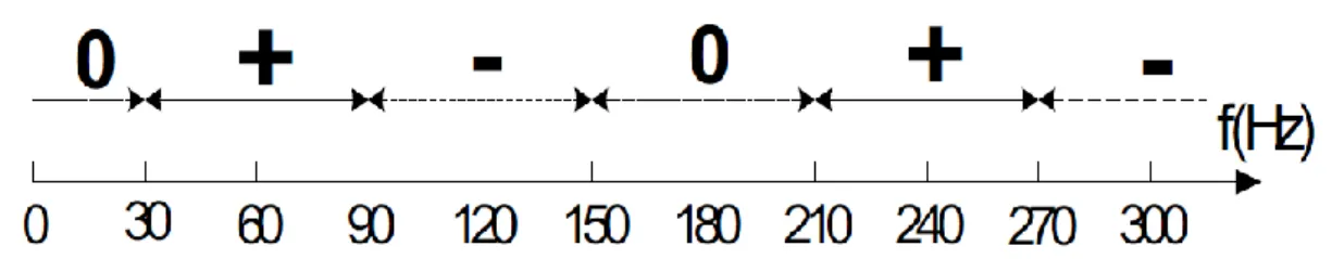
20 Figure 2.6 presents the pictorial of sequence dominant frequency that will be adopted in the frequencies grouping process.

Figure 2.6 - Sequence dominant frequency bands for a 60 Hz power system. Source: Chang et al., (2004).

The frequency components located in a sequence dominant frequency band have similar sequence characteristics: for example, either, the positive, negative or zero sequence is dominant. Therefore, the sequence dominant frequency band (𝑁 − 0.5)𝑓0 to (𝑁 + 0.5)𝑓0

Hz can be chosen as the frequency band of a group of frequencies. The physical meaning of a group frequency (GF) is that a GF is an equivalent component of all the frequency components located in a given sequence dominant frequency band based on the same power quality impact (Chang et al., 2004).

Given that each GF has two defining parameters, the second stage of characterizing the method is to determine these parameters, which are, the amplitude and frequency of the GF. The amplitude is determined according to equation (2.4), where ℎ is taken over 𝑓1 <

𝑓 ≤ 𝑓₂, where 𝑓₁ and 𝑓₂ are the frequencies that limits the group inferiorly and superiorly respectively (Oppenheim and Schafer, 2010).

𝑉

_{= √∑ 𝑉}

ℎ

(2.4)

Where,

21 By employing equation (2.4), the GF have the same total harmonic distortion (THD) as all the frequency components. The frequency of a GF is calculated utilizing the specific power quality index 𝐾, as described in equation (2.5) (Chang et al., 2004).

𝑓

= √𝐾𝑓

Where,

𝐾 is the K-factor calculated over the frequency band as presented in equation (2.6).

𝐾 =

∑

[

𝑓

𝑓

𝑉

]

∑

𝑉

Where 𝑁 is the number of frequency components in a load current.

It is noted that the group frequency is now weighted by the magnitude, which allows 𝑓𝐺(𝑓1, 𝑓2) in approaching the most relevant individual frequency component, within the

stipulated limit.

A sequence dominant frequency band is used to decide the frequency band of a GF, i.e. if frequency 𝑓₁ and 𝑓₂ are the two border frequencies, the GF located in the selected frequency band will have the characteristic of the dominant sequence. Therefore, the frequency of the GF could be between the border frequencies 𝑓₁ and 𝑓₂.

2.6 - ALGORITHMS FOR SIMULATING THE GROUPING METHODS

In this section, the algorithms developed for the application of the original waveforms, in other words, the waveforms with real characteristics and the algorithms responsible for performing the groupings according to the IEC standard and Chang will be presented. Then, the applications of the reconstructed waveforms from the resulting spectra of these

22 groupings will also be present in the course of the algorithms.

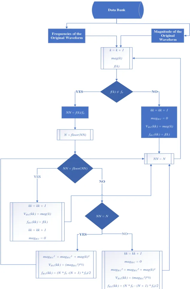
Figure 2.7 and 2.8 respectively show the grouping algorithms according to the IEC and Chang grouping methods in the form of a block diagram.

It is worth mentioning that the adequacy of these algorithms was examined and thus making it possible to validate them before their implementation in this study.

23 Frequencies of the Original Waveform Magnitude of the Original Waveform k = k + 1 mag(k) f(k) f(k) f0 NN = f(k)/f0 kk = kk + 1 magIE C = 0 VIE C(kk) = mag(k) fIE C(kk) = f(k) N = floor(NN) NN = N NN = floor(NN) kk = kk + 1 VIE C(kk) = mag(k) fIE C(kk) = f(k) kk = kk + 1 magIE C = 0 NN = N

magIE C² = magIE C² + mag(k)² VIE C(kk) = (magIE C²)^½ fIE C(kk) = (N * f0 -(N + 1) * f0)/2

kk = kk + 1 magIE C = 0 magIE C² = magIE C² + mag(k)²

VIE C(kk) = (magIE C²)^½ fIE C(kk) = (N * f0 – (N + 1) * f0)/2 Data Bank YES NO YES NO NO YES

24 Frequencies of the Original Waveform Magnitude of the Original Waveform k = k + 1 mag(k) f(k) f(k) f0

NN = floor(30 +f(k)/180) VChan g(1) = mag(k) fChan g(1) = f(k) NN = N NN = N k k [mag(k) * (f(k)f0)]² k k mag(k)² k0 = k k fChan g(kk) = (k0)^½ * f0

magk0 = magk0 + mag(k)²

VChan g(kk) = (magk0)^½ (3*N + 0.5)*f0 f(k) (3*N + 1.5)*f0 k k [mag(k) * (f(k)f0)]² k k mag(k)² k1 = k k fChan g(kk) = (k1)^½ * f0

magk1 = magk1 + mag(k)²

VChan g(k + 1) = (magk1)^½

k k [mag(k) * (f(k)f0)]²

k k mag(k)²

k2 = k k

fChan g(kk + 2) = (k2)^½ * f0

magk2 = magk2 + mag(k)²

VChan g(k + 2) = (magk2)^½ Data Bank YES NO YES (3*N - 0.5)*f0 f(k) (3*N + 0.5)*f0 kk = kk + 3 k k k k magk0 = 0 k magk1 = 0 k magk2 = 0 (3*N + 1.5)*f0 f(k) (3*N + 2.5)*f0 Yes No Yes No NO

25 From Figure 2.7, it can be observed that the IEC algorithm has three parts: the grouping of interharmonics, the separation of harmonics and the separation of the fundamental frequency. Moreover, from Figure 2.8, it can be seen that the Chang algorithm has two important parts: the grouping of interharmonics according to the predominance of the symmetric components (positive, negative or zero sequence), and the separation of the fundamental frequency.

Where:

k is the scanning counter of the original frequency spectrum;

kk is the counter of the frequencies obtained in the grouping process;

𝑓₀ is the fundamental frequency of the system;

The loop will only end with the finalization of the original frequency vector counting;

floor () is a SCILAB command that allows the rounding of any number to its own integer;

All variables in the IEC algorithm were initialized at 0. Meanwhile, in the Chang algorithm, all variables were initialized at 0 except for kk which has a value of 2 attributed to it.

2.7 - FINAL CONSIDERATIONS

In this chapter, the causes and effects of harmonic and interharmonic distortions were initially discussed. Secondly, the spectral estimation method was briefly introduced. Then, a detailed discussion on the IEC and Chang grouping methods under evaluation in this study was presented. Ultimately, the algorithms that will be used for simulating the IEC and Chang grouping methods were exhibited in the form of a block diagram.

26

3 - EXPERIMENTAL APARATUS AND METHODOLOGY

3.1 - INITIAL CONSIDERATIONS

This chapter aims to present the experimental apparatus and the procedures adopted to perform the analysis of the spectral component grouping methods and the identification of which, based on laboratory tests, best represent the effects of harmonics and interharmonics on the current and temperature of a TIM. To this end, all the laboratory tests carried out in this study are described in detail here, considering two topics:

 The proposal of the data banks contemplating diverse interharmonic frequencies and harmonic orders; and

 The presentation of the procedures employed for evaluating the currents and temperatures of the TIM, as well as the strategies taken for comparing the IEC and Chang spectrum grouping methods.

In order to approach the adopted measures, the experimental apparatus used to carry out these procedures is presented.

3.2 - EXPERIMENTAL APPARATUS

A necessary condition for the realization of this study is that the harmonics and interharmonics signals are generated and adjusted automatically. To meet this demand, an input signal control and reporting tool, developed in (Silva M.D. et al., 2017), that contains the readings of the numerous values relevant to the motor was designed and cultivated in the laboratory. This system was then improved in this study for applications involving interharmonics. Figure 3.1 illustrates the said system.

27 Figure 3.1 - Scheme of the control system and quantities report generation. Source:

Silva M.D. et al., (2017).

It can be seen from Figure 3.1 that the experimental apparatus consists of several elements. The following is a brief presentation of each of these elements.

 Input Data: a text file sequentially containing the duration, reference voltage values and a limit for the feeding currents of the TIM;

 CSW11100 Programmable California Instrument Power Source: responsible for generating the harmonics and interharmonics signals as well as the input voltages for feeding the TIM through commands from the connected computer;

 Elspec Model G4500: performs the various electric readings used to feed the TIM. This device has its own software for acquiring its readings. However, the program is not used in this study. The control system performs the readings in real time through the RS-422 standard and employs the Modbus protocol;

 NI PCI-6251 National Instruments Data Acquisition Board: carries out voltages readings with high sampling rate and accuracy, and has a pulse counter. This board is

28 responsible for reading the values of the sensors for their subsequent transformation into physical quantities. It has an internal DC voltage source of 5 V;

 PT-100 Type Temperature Sensors: these are the three sensors installed in the stator windings of the TIM. The resistances of the sensors vary in a known manner as a function of the temperature. They are read by adding a 2-kΩ low thermal coefficient resistor in series with each of the PT-100. Thus, they form three voltage-dividing circuits. Finally, with the use of the 5 V DC source of the data acquisition board feeding each voltage divider circuit, it is possible to obtain the values of the resistances of the PT-100s by applying the basic electric circuit equations;

 MKDC-10 Model Torque Sensor: is powered by a 10 V independent DC voltage source. The output voltage is in the order of millivolts. It varies depending on the torque;

 HS35B1024 Series Veeder Root Incremental Encoder: fed by a 5 V independent DC voltage source from the data acquisition board. At each turn, the encoder generates 1024 square wave pulses. The rotation speed is obtained by using a counter and identifying the elapsed time between each reading;

 Three-Phase Induction Motor: this machine has the PT-100 temperature sensors in the three phases of its stator windings. It is coupled to a DC generator and has a service factor of 1.15, rated power of 1.5 kW, and rated current of 3.56 A for a wye connection;

 Linear Current Voltage Regulator: this is a device developed in the laboratory. This regulator is required so that changes in the voltage level of the network do not affect the feeding of the DC generator field coil. In addition, the voltage regulator has filters that reduces the ripple factor of the voltage wave;

 DC Current Generator of 4 kW: serves as a linear load. The DC voltage regulator in series powers its field coil with a variable resistance, allowing small adjustments in the voltage level. Its armature is connected to a variable resistive load. The values that the two variable resistors must assume are those that result in the nominal currents of

29 the TIM when it is fed with balanced and steady state voltages. These values must be kept unchanged during all tests;

 Computer: Controls and processes all the information, communicates with the programmable source, with Elspec, and with the data acquisition board. All the programming was done in the NI LabVIEW Student Edition graphical development environment. The software initially receives the input data, and then enters a closed reading cycle of the quantities, comparing them with the reference values, and if necessary, sending command with new voltage values to the power source; and

 Acquisition System Report: Every three seconds of data acquisition, a new line is generated with the average values of all measured quantities. However, it is updated every 20 seconds. The report is saved in the text file format with the readings separated by tabulations, thus allowing easy conversion to a spreadsheet.

3.3 - DATA BANKS

In order to meet the objective of this dissertation, which is to analyze two frequency- grouping methods and identify which, based on laboratory tests, best represent the effects of harmonics and interharmonics on the currents and temperatures of a TIM, it is necessary to employ data banks that contemplates numerous interharmonic frequencies and various harmonic orders.

In this section, the conditions that will constitute the data banks are defined through the magnitude and phase of each frequency component.

3.3.1 - Definition of the Data Bank

In light of covering the highest and divers number of possible interharmonic frequencies, a database with 3,459 interharmonic and harmonic conditions is generated. However, the application of all these values to the TIM, considering the time sufficient for the motor to

30 reach thermal equilibrium1_{, makes it impossible to perform the laboratory procedure for}

all this conditions.

For this reason, in order to execute the 3,459 interharmonic and harmonic conditions, the electric currents circulating the stator windings are initially measured. Thus, the dwelling time in each condition is reduced to 50 seconds, sufficient to obtain the currents.

With the measured electric currents, 1,030 conditions, which will be subjected to the TIM to obtain its temperature at thermal equilibrium, are randomly selected from the previous 3,459 conditions. These conditions were selected in a way that they contemplate various conditions.

Seeking to provide a better understanding of the analysis and procedures performed in this work, the values adopted in each of the data banks under which the TIM is submitted in each stage of the tests will be described in details in the next sections.

Table 3.1 exhibits the data bank containing the various interharmonic frequencies and harmonic orders that the TIM will be subjected to. In sequence, a detailed explanation on how these data banks are applied to the TIM is presented.

1_{The definition of thermal equilibrium and the determination of a time value to reach it}

are characterized as a complex subject and depends on the size of the electric machines involved (electric motor and generator). In engineering, it is customary to define the settling time as the time required for the response curve to reach and remain within a 2% range around the final steady state value.

Based on practical results, it was verified in this study that a time of 16 minutes is enough to reach thermal equilibrium, as long as the variations in the interharmonic frequencies are smooth. In addition, the motor-generator set, at the beginning of the application of the interharmonic conditions, is already in steady state (such precautions are taken to carry out the tests).

31 Table 3.1 – Data Bank 1: Interharmonic frequencies and harmonic orders applied to the

TIM Data Bank 1

Group 1

Low and High Interharmonic Frequencies Magnitudes (%) Low Interharmonic Frequencies: 20 Hz - 183.5 Hz -

20 Hz - 30 Hz 1.5, 2.5 & 3

34.5 Hz - 55.1 Hz 2, 3 & 3.5

68 Hz - 183.5 Hz 3, 5 & 7

High Interharmonic Frequencies: 541 Hz – 2400 Hz 3, 5 & 7

Group 2

Interharmonic Frequencies and Harmonic Orders - Individual Interharmonic Frequency: 20 Hz - 2400 Hz 3

Individual Harmonic Order: 3rd_{, 5}th_{, 7}th_{, 11}th _{& 13}th _{3, 5 & 7}

Two Harmonic Orders: 3rd & 5th, 3rd & 7th, 3rd & 11th, 3rd & 13th, 5th & 7th, 5th & 11th, 5th & 13th, 7th & 11th, 7th & 13th _{and 11}th _{& 13}th_.

3 & 5, 3 & 7 and 5 & 7

3.3.2 - Data Bank 1 (𝑫𝑩_𝟏)

Data Bank 1 (𝐷𝐵₁) is the main data bank used in this study to analyze the spectral component grouping methods that best represent the effects of harmonics and interharmonics on the temperature of the TIM. This data bank covers a wide range of interharmonic frequency conditions (20 Hz – 2400 Hz). The interharmonic frequencies and harmonic orders used in this data bank alongside with the magnitudes can be seen in Table 3.1.

The 𝐷𝐵₁ is composed of two groups (Group 1 and Group 2). Group 1 consists of the combination of 28 individual low-interharmonic frequencies ranging from 20 Hz – 183.5 Hz with 28 individual high-interharmonic frequencies ranging from 527 Hz – 2400 Hz. Here, the frequencies between 20 Hz and 30 Hz are combined with magnitudes of 1.5%, 2.5% and 3% independently, while the frequencies between 34.5 Hz and 55.1 Hz are combined with magnitudes of 2%, 3% and 3.5% individually. The frequencies above 60 Hz are combined with magnitudes of 3%, 5% and 7% independently. The total number of conditions in this group is equal to 84.

32 Moreover, group 2 comprises of 75 individual interharmonic frequency from 20 Hz – 2400 Hz with magnitudes of 3%, combined with 5 individual harmonics of the 3rd_{, 5}th_,

7th_{, 11}th _{and 13}th _{orders, which are individually combined with magnitudes of 3%, 5% and}

7% (a total of 15 individual harmonic conditions) and 75 individual interharmonic frequency from 20 Hz – 2400 Hz with magnitudes of 3% combined with a group of two harmonic having different combination of the 3rd, 5th, 7th,11th and 13th orders, and also with combined magnitudes of 3%, 5% and 7% (a total of 30 conditions with group of two harmonic). The total number of conditions in this group is 3,375.

It is worth noting that the selection of the frequencies in the range specified in 𝐷𝐵₁ (20 Hz – 2400 Hz) is arbitrary. However, this range was selected considering the following facts observed in the literature: a) for interharmonic frequencies greater than that of the power frequency heating effect are observed in the same fashion as those caused by harmonic currents (IEEE interharmonic task force, 2001); b) at interharmonic frequencies twice higher than the power frequency, the modulation impact on the rms value is small compared to the impact in the frequency range below the second harmonic (Interharmonic task force, 2001) and c) at steady speed of the motor, the frequencies of the disturbing components are usually in the range of 500 Hz – 2000 Hz, but during the startup period, this range might expand significantly (Hanzelka and Bien, 2004).

3.3.3 - Data Bank 2 (𝑫𝑩𝟐)

This data bank is constituted of 1,030 interharmonic frequencies and harmonic orders. The values of this data bank are used to identify the temperatures of the TIM.

In fact, the conditions in 𝐷𝐵₂ are contained in 𝐷𝐵₁. The difference between the results of the application of the interharmonic frequencies and harmonic orders in 𝐷𝐵₁ and 𝐷𝐵₂ on the TIM is due to the dwelling time set for each data bank during the tests. In 𝐷𝐵1, the

dwelling time between the start of the application of the condition and the data collection is equal to 50 seconds, which is insufficient for thermal equilibrium. However, in 𝐷𝐵₂, this time is equal to 16 minutes.

33 The selection of the 𝐷𝐵2 values is performed by means of a computational algorithm

developed in SCILAB. In order to obtain the 𝐷𝐵₂, the said algorithm selects from the 𝐷𝐵₁, the conditions whose modules of the electric currents are diversified. Then, the database is ordered so that there are no abrupt changes in the electric currents between consecutive conditions.

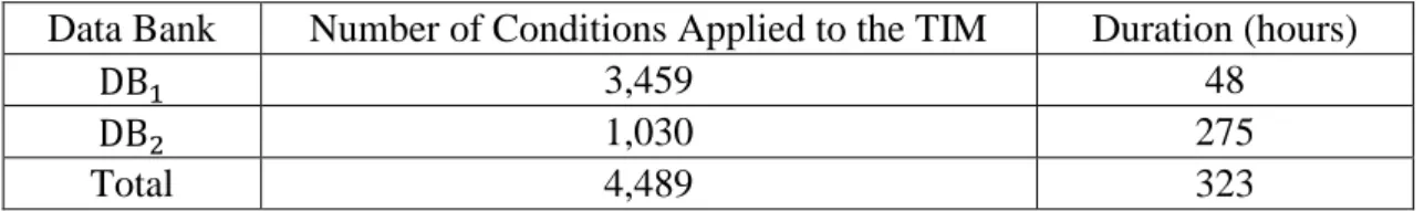
Table 3.2 shows the number of conditions imposed on the machine and the time spent, in hours, for each data bank.

Table 3.2 - Number of conditions applied to the TIM and the duration of each of the data bank

Data Bank Number of Conditions Applied to the TIM Duration (hours)

DB₁ 3,459 48

DB2 1,030 275

Total 4,489 323

As mentioned, the dwelling time of each condition consisting the 𝐷𝐵₁ is 50 seconds and 16 minutes for each condition in the 𝐷𝐵1, except for the first condition in both data banks

which has a dwelling time of 3 hours so as to ensure operation in steady state.

3.4 - PROCEDURES FOR COMPARING THE GROUPING METHODS

The comparative analysis of the grouping methods is divided into two parts. In the first part, the conditions in DB1 are used to measure the electric currents of the TIM. Then

from the conditions in DB2, the temperature of the TIM is measured.

The following procedures are adopted for the comparative evaluation between the grouping methods under analysis.

1. Generation of the original waveform; 2. Subjection of the TIM to this waveform;