Drivers of agricultural future commodity prices : a co-integration analysis

M

ASTER IN

F

INANCE

M

ASTER

´

S

F

INAL

W

ORK

D

ISSERTATION

DRIVERS OF AGRICULTURAL FUTURE COMMODITY

PRICES: A COINTEGRATION ANALYSIS

J

OÃO

F

ILIPE

M

ELO DE

A

LMEIDA

F

IGUEIREDO

M

ASTER IN

F

INANCE

M

ASTER

´

S

F

INAL

W

ORK

D

ISSERTATION

DRIVERS OF AGRICULTURAL FUTURE COMMODITY

PRICES: A COINTEGRATION ANALYSIS

J

OÃO

F

ILIPE

M

ELO DE

A

LMEIDA

F

IGUEIREDO

O

:

P

P

J

M

H

Abstract

This dissertation aims to study the effects of changes in the prices of future contracts on Brent Crude Oil and US Dollar Index in the price of several agricultural future contract prices (Cocoa, Cotton, Coffee, Sugar, Soybean, Wheat and Corn).

These futures outrights are traded on ICE (Intercontinental Exchange, Inc.) and have a remarkable liquidity. Weekly data was used from March 2013 to March 2015 with a total of 105 observations. The prices were collected from the Quandl futures database and are settlement prices from the front outrights. The Back-Adjusted method was chosen to perform the roll over.

We started by studying the correlation between US Dollar Index and Brent Crude Oil prices. Confirming the conclusions of other studies, we found a negative correlation between the prices of Brent Crude Oil and the US Dollar Index. The Granger Causality test gave us enough statistical evidence to conclude that a variation in Brent Crude Oil prices indeed cause an impact on the US Dollar Index.

By applying Johansen`s cointegration test we indeed found cointegrating vectors between Brent Crude Oil, the US Dollar Index and each one of the studied agricultural commodities. The next step was to build vector error correction models. Although some of them proved not to be rock solid, we manage to establish a link among the variables, namely in the case of Soybean, which produce remarkable results and may, in fact, be treated as a benchmark for traders of future contracts.

Keywords: Cointegration, Future Contracts, agricultural commodities, Brent Crude Oil, US Dollar Index

Acknowledgements

First, I would like to thank my supervisor Pierre Hoonhout for all the support and advices given along the process which undoubtedly contributed for the final outcome of this dissertation.

To my family, especially to my parents and to my brother, for the unconditional support they always gave me.

A special thanks goes also to my colleagues at OSTC for the daily support, knowledge sharing and motivation to pursue this topic.

Table of Contents

1 Introduction 1

2 Literature Review 3

3 The Data 7

4 Methodology 9

4.1 Stationary and non-stationary time series 9

4.2 Augmented Dickey-Fuller test 10

4.3 Cointegration 11

4.4 Johansen test 12

4.5 Granger Causality test 13

4.6 Akaike Information Criteria 14

4.7 VAR model, VEC model 14

5 Empirical Results 17

5.1 Relationship between Brent Crude Oil Prices and the US Dollar Index

21

5.2 Relationship between Brent Crude Oil price, the US Dollar Index and some agricultural commodities price

25

6 Summary and Conclusions 32

7 References 34

List of Tables

Table I - Critical Values of ADF test 18

Table II - Augmented Dickey-Fuller test (results in level) 18

Table III - Augmented Dickey-Fuller test (results in first differences) 19

Table IV - Johansen Cointegration Test output 21

Table V - Granger Causality Test output 22

Table VI - Vector Error Correction Model 23

Table VII - Breusch-Godfrey Serial Correlation LM Test and ARCH Test 24

Table VIII - Johansen´s trace test results 26

Table IX - Cointegrating vectors 27

Table X - Short Run Parameter Estimates 28

Table XI - Tests and Residual Diagnostics 29

Table XII - Optimal Lag Length Selection 37

Table XIII - Choosing appropriate model for VECM on Brent Crude Oil price

and US Dollar

38

Table XIV - Statistics from VECM (Brent Crude Oil – US Dollar Index) 39

Table XV - Johansen Test Results - Corn, Brent Crude Oil, US Dollar Index 40

Table XVI - Johansen Test Results - Sugar, Brent Crude Oil, US Dollar Index 40 Table XVII - Johansen Test Results - Coffee, Brent Crude Oil, US Dollar

Index

41 Table XVIII - Johansen Test Results - Cocoa, Brent Crude Oil, US Dollar

Index

41

Table XIX Johansen Test Results - Cotton, Brent Crude Oil, US Dollar

Index

42 Table XX - Johansen Test Results - Soybean, Brent Crude Oil, US Dollar

Index

42 Table XXI - Johansen Test Results - Wheat, Brent Crude Oil, US Dollar

Index

List of Figures

Figure 1 - Stationary and non-stationary time series 9

Figure 2 - Example of cointegrated time series, Bação (2000) 12

Figure 3 - Plot of Brent Crude Oil and US Dollar Index 17

Figure 4 - Graph of Δ Brent (Brent Crude Oil first differences) 20

Figure 5 - Jarque-Bera residual test 24

Figure 6 - Response of US Dollar Index to a shock in Brent Crude Oil Price 25 Figure 7 - Response of Soybean prices to a shock in US Dollar Index and in

Brent Crude Oil price

30

Figure 8 - Response of Cocoa prices to a shock in US Dollar Index and in Brent Crude Oil price

31

Figure 9 - Response of Sugar prices to a shock in US Dollar Index and in Brent Crude Oil price

31

1

1.Introduction

Trading is believed to have taken place throughout much of the recorded history of human kind and it is an important asset of our economy. Speculation played a key role in the development of financial markets and trading platforms.

From stocks to bonds, futures and options nowadays it is possible to trade hundreds of thousands of different financial products. With the flourishing of organized clearing houses and the generalization of electronic trading the financial markets have now more liquidity than ever and are at every person´s reach.

Having this context as starting point, this dissertation aims to test the presence of cointegrating relations between the prices of future contracts in Brent Crude Oil, US Dollar Index and agricultural commodities.

Exchange rates are known for their direct impact on the export and import of goods and services and, thus, are expected to influence the price of these trading commodities.

At the same time, the use of chemical and petroleum derived inputs has increased in agriculture over time. It is therefore expected that energy, namely the price of Crude Oil, to have an important impact in commodity production.

Working as a futures trader for OSTC Portugal, I find this topic deeply interesting and useful both in theoretical and practical framework.

The number of future contracts traded on exchanges worldwide is increasing every year and dozens of millions of contracts change hands every trading day.

2

According to FIA (Futures Industry Association), more than 12,1 billion future contracts were traded worldwide in 2014 alone. Agricultural commodities have also being flourishing in 2014, showing a volume increase of more than 15% from approximately 1,2 billion contracts traded in 2013 to 1,4 billion in 2014.

Many prior studies were conducted to test these relations between Crude Oil prices and agricultural commodities prices (Nazlioglu (2012)), between the US Dollar strength and agricultural commodities prices (Abbot et al. (2008)) and between the three variables (Harri et al (2009)) over a significantly long period of time using weekly or monthly data.

Trading future contracts is a highly leveraged investment. The initial margin required to enter into a new futures contract is usually lower than 10% of the futures contract.

This may bring a big profit (or loss) to an investor for a small market movement. In fact, many futures traders enter in a position to make 1 or 2 ticks (minimum amount prices of future contracts can move).

Therefore, this study will focus on a short-run analysis with weekly observations, which may lead to novel conclusions and serve as a benchmark for practical purposes.

3

2. Literature Review

Is there any relationship between exchange rates and Crude Oil prices and commodities prices? This subject has been studied by different authors in the last years. The purpose of their studies is mainly related to a practical need: to find a comprehensive model that explains past prices and predicts future prices of those commodities.

In fact, the fluctuation of Crude Oil prices ( by far the most traded commodity) and the volatility of some agricultural commodities (corn, wheat, soybean, for example) and also the exchange rate (mainly the US Dollar exchange rate, in comparison with other currencies, euro, yen, Australian dollar) tend to be correlated. How do they influence each other?

Novotni (2012) studied the relationship between the nominal effective exchange rate of the US Dollar and the Brent Crude Oil price, examining monthly data from January 1982 to September 2010. He modeled the Brent Crude Oil price as a function of some explanatory variables: nominal effective exchange rate of US Dollar, the industrial production of the OCDE countries and oil inventories of United States. He concluded that, in the period between 2005 and 2010, Brent Crude Oil price and the exchange rate were related in an inverse way: decreasing the nominal effective exchange rate of the Dollar of 1% implies an increase in the Brent Crude Oil price of 2,1%. Before 2005 the correlation between those two variables was very weak or even inexistent.

One explanation for the inverse relation between Brent Crude Oil price and the effective exchange rate of the US Dollar may be the fact that commodities are traded in US Dollar, so depreciation in US Dollar implies the compensatory rise of the commodities price.

4

Natalenov et al (2013) studied the relationship between Crude Oil, corn and ethanol during a particularly turbulent period between 2006 and the end of 2011.

Their first conclusion was that, considering the whole period of time, there was no correlation between these three variables. Then the period of time was divided in two sub periods, the first from March 2005 to July 2008, and the second period of time from August 2008 to the end of 2011. At the same time, they decided to look for a bi-variate relation between two variables, instead of looking for cointegrated relations between the prices of the three mentioned commodities.

They came to the conclusion that, between 2008 and 2011, the Brent Crude Oil price and corn, and the Brent Crude Oil price and ethanol, were linearly related, with changes of the Brent Crude Oil price implying changes, with the same signal but with different amplitude, on the corn and the ethanol prices.

Natalenov referred to some factors that may have contributed to the complex relation between those three commodities prices: The Energy Policy Act of 2005, Crude Oil price level surpassing the threshold of 75 USD/barrel and the 2008 financial crises.

Nazlioglu (2012) analysed the price transmission from the world oil prices to the key agricultural commodity prices by employing weekly data from 1994 to 2010. Using Granger causality test, Nazlioglu found empirical evidence of a nonlinear causal linkage between Oil and the agricultural commodity prices for corn, soybean and wheat.

Another study on this topic was put forth by Campiche et al. (2007). This research examined the co-variability between Crude Oil prices and corn, sugar, sorghum, soybeans, soybeans oil and palm oil prices during the period 2003-2007. Johansen cointegration tests revealed no cointegrating relationships during 2003-2005, but a

5

positive cointegration of corn prices and soybean prices with oil prices during the 2006-2007 time periods.

Abbot et al. (2008) highlights the strong and important link between the US Dollar Index and commodity prices. Most commodities are priced in US Dollars, but are purchased in the local currency. When the dollar strength falls there is a link with rising commodity prices.

A similar approach is used by Murphy (1999). By graphically illustrating a similar path between gold prices and the US Dollar Index from April 1995 to October 1996, it states that a rising Dollar normally has a depressing effect on most commodity prices.

Harri et al (2009) studied the relationship between the exchange rate (measured as a trade weight average of the US dollar value against other major currencies), Crude Oil price and some other commodities (mainly corn, cotton and soybeans) prices. By using overlapping time periods taken from monthly data, between January 2000 and September 2008, they found a cointegration relationship: oil prices are linked to corn, cotton and soybeans, but not to wheat.

They also found that the exchange rates, crude oil and corn prices are correlated, and that exchange rates influence the linkage of the commodities prices over time.

Rosa et al (2012) have studied the relationship between some agricultural commodities and crude oil prices, trying to test the hypothesis that the increased volatility in agricultural prices is caused by the exogenous crude oil prices. They used data between January 1999 and May 2012, and this study compared the prices of corn, wheat and soybean (whose choice is justified because they are the most traded agricultural commodities used on feedstock, food and fuel) with the crude oil price.

6

The authors concluded for a strong non-linear linkage between crude oil and corn prices, explained by the increased use of corn in the production of ethanol. The volatility of the crude oil price causes some volatility on corn and soybean prices, too, because of their energy and industrial use. The case of wheat prices is different: an increase in consumption leads to the decrease in wheat stocks, which is responsible for the large increase in wheat prices, during that period of time.

Zhang (2013) used Granger causality test to test the hypothesis that changes on the price of crude oil causes the change in the US dollar exchange rate, and not vice-versa. Golub (2013) explains that effect saying that when the oil price rises, it increases the income of oil exporting countries and those countries use the higher income to purchase more US dollars, which causes its appreciation. Using monthly data between January 2003 and June 2010, Zhang finds no evidence of significant cointegration between the two mentioned variables, but that evidence appears when allowing for two structural breaks in the past: November 1986 and February 2005 (these two dates are related with important changes in the oil market). He finally concludes that there is a stable relationship between the price of Crude Oil and the value of the US dollar exchange rate, but that relationship has been subject to structural breaks over time.

7

3. The Data

The data used in this study is the Quandl Future prices database and comprises of weekly data (Tuesday) from the first trading Tuesday of March 2013 until the first trading Tuesday of March 2015 with a total of 105 observations per product.

The variables used are futures in Brent Crude Oil, US Dollar Index, Corn, Soybean, Wheat, Cocoa, Coffee C, Cotton and Sugar No.11.

The US Dollar Index is a measure of the value of the US Dollar relative to a basket of foreign currencies. It is calculated as a weighted geometric mean of Dollar´s value against Euro, Japanese Yen, Pound Sterling, Canadian Dollar, Swedish Krona and Swiss Franc. In the future markets, one contract is traded as 1000$ x Index Value.

All the prices collected are settlement prices, which is a trade weighted average of the number of lots traded at each price over a certain period of time, shortly before the close of the market. This price is used to determine the profit or loss for the day in order to update margin requirements.

All these future prices are from the Intercontinental Exchange (ICE), a leading network of exchanges and clearing houses for financial and commodity markets, which operates completely as an electronic exchange.

One important aspect that we face when dealing with future contracts is the expiring nature of the product.

Futures are not continuous contracts such as stocks. Each specific contract has a starting trading day and an expiring day. For this reason, it is essential to use a roll method

8

between contracts to create a continuous future contract which can later be used for back testing.

Stringing subsequent price series together creates a discontinuous time series since the expiring of a contract and the passage to the next front-month may carry significant price gaps.

Therefore, the roll method used in this study is the Back-Adjusted method. The gap between two contracts is measured, and then added or subtracted to all values in the prior contracts.

This method is one of the most commonly used for this purpose, being also used by CQG Trader, a leading high-performance market data and electronic trading application used by future traders worldwide.

This work has been made of attempts and reformulations depending on the results and difficulties, which were found throughout the process. However, it was carried out the usual approach in this type of work: the sources and the data to be used were selected; the next step was to verify whether the data presented some kind of correlation (a look on the plot of the data is useful to this purpose) and run some tests concerning that correlation. The third step was to find a model that could express the evolution in time of the variables which were to be studied in order to fit the purpose of this analysis: try to understand in what sense agricultural commodities prices are related with the exchange rate and the Brent Crude Oil price.

The statistical software used to conduct this research was EViews. We´ve choose EViews because it is commonly used in statistical works and provides all kind of tests, models and tools that should be necessary.

9

4. Methodology

This section discusses theoretical principles used in this work.

4.1. Stationary and non-stationary time series

Gujarati (2011) refers that “a time series is said to be stationary if its mean and variance are constant over time and the value of the covariance between the two periods depends only on the distance or gap or lag between the two time periods and not the actual time at which the covariance is computed” . However, many time series, more exactly typically financial time series, often display some kind of systematic upward or downward movement through time and, as a consequence, are not stationary.

Stationary and non-stationary time series demand different approaches, otherwise forecast studies will predict, most probably, inconsistent conclusions and unrealistic or divergent results. A time series with a trend is one of the most usual examples of non-stationary time series.

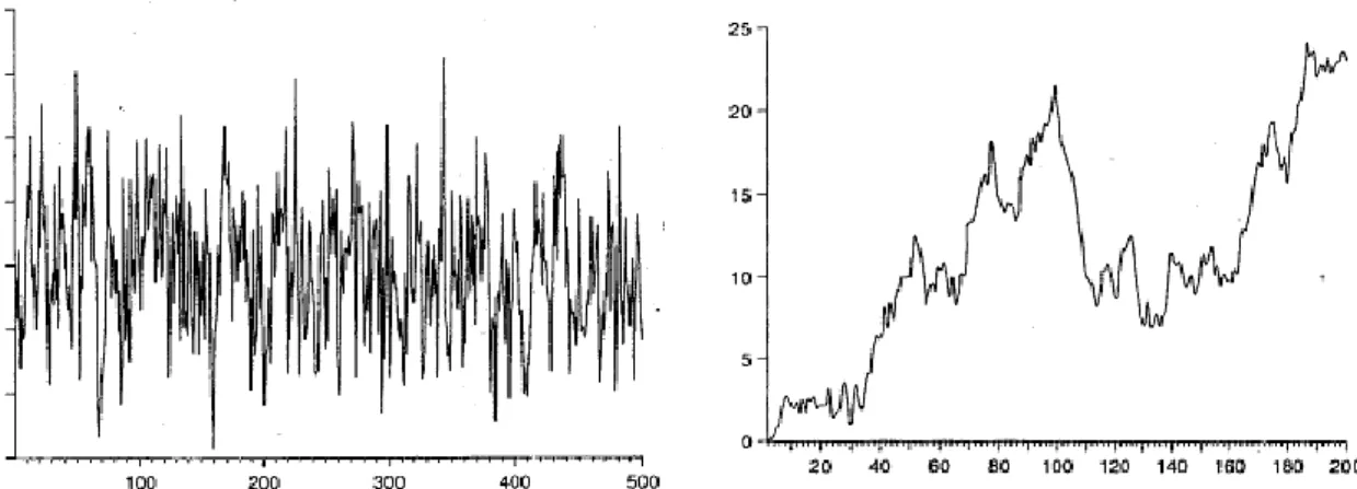
Figure 1 illustrates a stationary and a non-stationary time series.

FIGURE 1: stationary time series and non-stationary time series, respectively (Asteriou, 2007)

10

If the series has a deterministic long-run trend it may be possible to transform it into stationarity, by considering the deviations from the trend. If the trend is stochastic, transformation into stationarity requires first-differencing.

Only rarely is differencing more than once necessary to obtain stationary time series.

4.2. Augmented Dickey-Fuller (ADF) test

To test the stationarity of a time series we usually use the reference test or the Augmented Dickey-Fuller test.

Dickey and Fuller proposed three alternative regression equations, based on a simple AR(1) model, that can be used for testing for the presence of unit root as synonymous of non-stationarity.

These equations are: y_t y_t1u_t (1) y_t y_t1u_t (2) y_t ty_t1u_t (3) Where (3) includes a time trend and a constant and (2) only includes a constant.

DF test is a t-test, but not a conventional one, so we must use non standard critical values which were first calculated by Dickey and Fuller, and later by other authors.

Dickey and Fuller extended their test procedure including extra lagged terms of the dependent variable. This allows for the testing of unit roots in autoregressive processes that are of order higher than one,

11

The three possible equations of the test are the same but now they all include the additional

term



i 1i. yt i. So we have the Augmented Dickey-Fuller test, with the null hypotheses

defined as Ho: there is a unit root.

This test may be used with all the variables and, when non-stationarity is observed, it may be used again to test their first differences, second differences, and so on.

We say that a variable is integrated of order 1, or simply I(1) when the series is non-stationary in level but his first differences are non-stationary.

4.3. Cointegration

If we have two or more non-stationary time series, that become stationary when differenced, such that some linear combination of those series is stationary, then we say that they are cointegrated. That means that those series show some kind of long-run relationship.

In other words, we say that two I(1) time series x and _t y are cointegrated, if there is a _t  such that z_t  y_t .x_t is stationary.

Figure 2 illustrates the situation: x and _t y are non-stationary, but in long-run they are _t

moving together. So we may find a relation between those two series, and define a third one which is stationary.

12

FIGURE 2: Example of cointegrated time series, Bação (2000)

In this example, if we suppose that z is approached by_t x_t 2.y_t, for instance, then (1,2)

will be a cointegrating vector between the variables x and_t y . More generally, the _t

cointegrating vector is a (k,2k) vector (k 0).

4.4. Johansen test

To test the existence of cointegration between the variables, we may use, at least, one of three kind of tests: the Engle-Granger cointegration test developed by Engle and Granger (1987), the Philips-Ouliaris reference test, presented by these authors, or most recently the Johansen cointegration test, presented by Johansen and Juselius in 1990.

The main advantage of the Johansen test, regarding the others tests, consists in the determination of the number of cointegrating vectors that exists among the studied variables, when these variables are cointegrated, and provides estimates of all cointegrating vectors.

As Dwyer (2014) refers, the Johansen test can be seen as a multivariate generalization of the ADF test because it is the study of linear combination of variables for unit roots. It must be noticed that if there are n variables, each with unit roots, there are n1 possible

co-13

integrating vectors, and if there are nvariables and n cointegrating vectors, then we may conclude that the variables do not have unit roots.

Johansen proposes two different tests: the trace test and the _maxtest.

The trace test is based on the log-likelihood ratio ln[L_max(r)/L_max(k)] and is conducted sequentially for r k1,...,1,0. This test tests the null hypothesis that the cointegration rank is equal to r against the alternative hypothesis that the cointegration rank is equal to k .

Asteriou (2007) refers four steps in Johansen test approach: step 1: test the order of integration of all variables; step 2: set the appropriate lag length of the model. This may be done using some criteria that we will see next; step 3: choose the appropriate model that correlates the variables; step 4: determine the rank of  or the number of cointegrating vectors, using _maxtest or trace test.

4.5. Granger causality test.

We may test the possibility of statistical precedence between them: which one causes the other one movement? We may test it in both directions, using the Granger causality test.

Given two sets of time series data, x and _t y , we may create two models to test which of _t

them better fits to predict y : one model only with past values of _t y and the other model _t

with past values of y and _t x . _t

The residual sum of squares errors is compared and a test is used to determine which model is more adequate to explain the future values ofy . The null hypothesis is: H_t 0: αi = 0 for

14

each i, with _i the coefficient of the variablex , in the model, against H_t a: αi ≠ 0 for at least

one of the _i coefficients. We may execute this test using different values of lags.

4.6. Akaike Information Criterion

We must compare the goodness of fit data-models, to decide the number of lags must be used in the model. We may use some criteria provided by R or EViews software, for instance: the Akaike Information Criterion (AIC), the Finite Prediction Error (FPE), the Schwarz Baysean Criterion (SBC) and the Hannan and Quin Criterion (HQC).

Ideally the chosen model should be the one which minimizes all these criteria. However, sometimes the results are contradictory, and in the analysis of time series the statistic most commonly used is AIC. It is defined by:

n k e n RSS AIC 2         (4)

where we must recall that



  n t t û RSS 1 2

and û represents the difference between the actual _t

t

y and the fitted values predicted by the regression equation.

4.7. VAR (Vector Autoregressive) model, VEC (Vector Error Correction) model

We may model a time series data using some models. The simplest one is the autoregressive of order one model AR(1), which is given by:

15

Where  <1 and u is a Gaussian error term. This model assumes that the actual value of _t

t

y is determined by its own value in the precedent period.

The model becomes more complex when we have more than one time series, with the actual values of each one influenced not only by its own past values, but also by the past values of all the others variables. In this case we can use a VAR model.

Pfaff (2006) defines a Vector Autoregressive model as a set of k endogenous variables written in the form:

u p t p t t Ay A y u y  1 1 ...   . (6)

In this equation, A is the (_i kk) matrix of coefficients and u is a k-dimensional lagged _t process of order p, with E(ut)0.

More clearly, considering two variables, we may write it in the following way:









where we assume that u_1t and u_2t are uncorrelated white-noise error terms, called impulses or

shocks.

In this form we may see that y and _t x are affected not only by their past values, but each _t

variable is affected, too, by the other variable past and current values.

Although the number of lagged values of each variable can be different, we usually use the same number (p) of lagged terms in each equation

16

A VAR model can be reformulated as an error correction model considering the following relation:

y_t y_tp ₁y_t1..._p1y_tp1u_t , (9)

With .'. The matrix is the loading matrix (includes the speed of adjustment to equilibrium coefficients) and the coefficients of the long-run relationships are contained in', and the _i matrices measure the effect of transitory impacts.

The (kk) 'matrix contains the error correction terms. The dimensions of  and  are k and r , respectively, and r is the number of long-run relationships between the variables y do _t

exist.

The general case of VECM including all the options is:

. 1 1                 t y [y_t1 1 t ] ₁y_t1..._k1y_tk1₂₂tu_t (10)

where the terms represent: ₁: intercept in the cointegrated equation (CE), ₁: trend in CE; ₂: intercept in VAR; ₂ : trend in VAR. EViews provide us with five distinct models depending on the existence of intercept and trend in CE or in VAR; the model with trend in CE and in VAR is only theoretical (non realistic) so, in practice, it is rarely adopted.

In VECM model, the rank (or trace) of matrix 'has the following lecture, concerning with the cointegration of the variables: if r 0 there is no cointegration (we can’t use VECM, only VAR in first differences); if 0rk there are r cointegrating vectors (we can use VECM); if

k

17

5. Empirical results

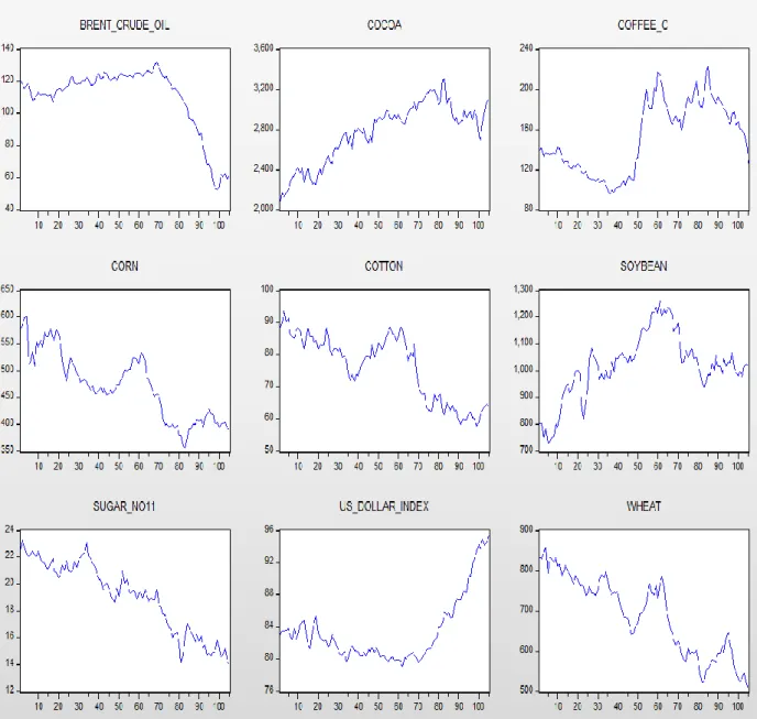
A regard over the plot of the time series data may pronounce the existence of temporal correlation amongst the variables (Figure 10). Some of them are expected to be correlated (Corn and Brent, for instance, according to some literature) but the nature of this study, mainly focused on short-run prices, may produce unexpected results.

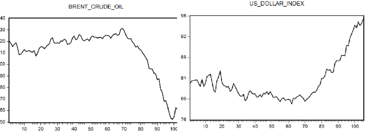
Figure 3 shows the plot of Brent Crude Oil and the US Dollar Index during the studied period. It is not clear the existence of cointegration; in fact, cointegration, seen as a long-run relationship, may not be seen in a two years time period, with weekly observations.

FIGURE 3: Plot of Brent Crude oil and US Dollar Index.

As it was mentioned before, it is necessary a preliminary study of stationarity of the variables. This study may begin by the observation of the plot of the time series and, next, by the application of the ADF test. To run this test we may begin fitting a model, chosen among the three options (none, intercept or trend) and a regard over the plot may be an important step. In order to avoid spurious regression problem, we will begin

18

searching for unit roots using the ADF test with the options and compare the results with the ADF critical values, provided by EViews (Table I)

TABLE I

Critical values to ADF test, taken from Hamilton (1994) and Dickey and Fuller(1981)

Significance level 1% 5% 10%

Model

Constant -3,500 -2,892 -2,583

Constant and trend -4,059 -3,454 -3,153

None -2,588 -1,944 -1,615

The Augmented Dickey-Fuller test is preceded by the determination of the optimal number of lags, and that was made using the Akaike Information Criterion.

The results of the t-test are contained in tables II and III, with reference to the fitted model and the number of lags.

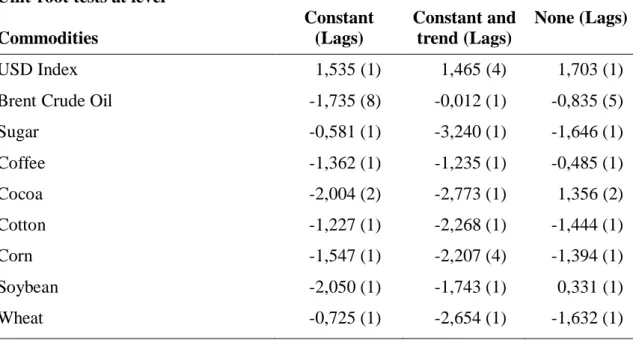
TABLE II

Augmented Dickey-Fuller test (results in level) Unit-root tests at level

Commodities Constant (Lags) Constant and trend (Lags) None (Lags) USD Index 1,535 (1) 1,465 (4) 1,703 (1)

Brent Crude Oil -1,735 (8) -0,012 (1) -0,835 (5)

Sugar -0,581 (1) -3,240 (1) -1,646 (1) Coffee -1,362 (1) -1,235 (1) -0,485 (1) Cocoa -2,004 (2) -2,773 (1) 1,356 (2) Cotton -1,227 (1) -2,268 (1) -1,444 (1) Corn -1,547 (1) -2,207 (4) -1,394 (1) Soybean -2,050 (1) -1,743 (1) 0,331 (1) Wheat -0,725 (1) -2,654 (1) -1,632 (1)

19

TABLE III

Augmented Dickey-Fuller test (results in first differences) Unit-root tests at first differences

Commodities (Lags) _None

USD Index (3) -7,266 Brent (4) -2,651 Sugar (1) -11,334 Coffee (1) -8,113 Cocoa (1) -8,554 Cotton (1) -10,481 Corn (1) -10,287 Soybean (2) -6,308 Wheat (1) -9,303

Comparing the values obtained, in Table II and III, with the critical values, in Table I, it is easy to conclude that all the variables are non stationary in level, at a statistical significance level of 5%, which is the usually adopted level. This is a no surprising result, after the regard of the plots of the studied variables. Figure 3 reveals the beginning of a particular turbulence period in the US Dollar Index and in Brent Crude Oil prices (October 2014- March 2015) and most of the agricultural commodities suffer the consequences of such volatility.

Next, the same test was run to the first differences of all the variables. In this case it was not necessary to test with the three models, because all the plots showed the values distributed more or less along the zero line, as we can see in Figure 4, with the graph of the Brent Crude Oil first differences.

20

FIGURE 4: Graph of Brent (Brent Crude Oil first differences)

In the case of the ADF test applied to the first differences, all coefficients are statistically significant at a 1% or lower level, which means that all the variables are integrated of order one:I(1).

Following the purpose of this study, next we will see if there is evidence of correlation in time among some variables. First we will test for correlation between Brent Crude Oil prices and the US Dollar Index as some previous studies (mentioned in the literature review) have done, in a larger temporal window. Then it will be studied the relationships among the US Dollar Index, Brent Crude Oil prices and each one of the agricultural commodities.

21

5.1. Relationship between Brent Crude Oil prices and the US Dollar Index

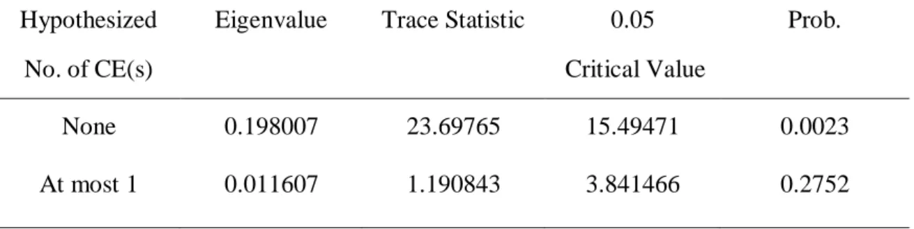
We can determine if Brent Crude Oil prices and the US Dollar Index are cointegrated using Johansen cointegration tests. Both tests (trace test and maximum eigenvalue test) reveal the presence of one cointegrating vector which describes the long run relationship between the two variables. The test output is in Table IV.

TABLE IV

Johansen Cointegration Test output

Included observations: 102 after adjustments Trend assumption: Linear deterministic trend Series: Brent Crude Oil; US Dollar Index Lags interval (first differences): 1 to 2

Unrestricted Cointegration Rank Test (Trace)

Hypothesized No. of CE(s)

Eigenvalue Trace Statistic 0.05

Critical Value

Prob.

None 0.198007 23.69765 15.49471 0.0023

At most 1 0.011607 1.190843 3.841466 0.2752

Unrestricted Cointegration Rank Test (Maximum Eigenvalue)

Hypothesized No. of CE(s) Eigenvalue Max-Eigen Statistic 0.05 Critical Value Prob. None 0.198007 22.50681 14.26460 0.0020 At most 1 0.011607 1.190843 3.841466 0.2752

22

Granger causality test was used to study the relationship between Brent Crude Oil prices and the US Dollar Index, with the optimal number of lags equal to 5 (Table XII). Table V shows that, in the period of time between March 2013 and March 2015, a change in Brent Crude Oil price indeed causes animpact in the US Dollar Index, but not the vice-versa.

TABLE V

Granger Causality Test output

Null Hypothesis Obs F-Statistic Prob.

ΔUS Dollar Index does not Granger Cause ΔBrent Crude Oil

99 0.64575 0.6654

ΔBrent Crude Oil does not Granger Cause ΔUS Dollar Index

4.42994 0.0012

Now it will be used the Vector Error Correction Model. Asteriou (2007) refers some reasons why this is a very useful model: it measures the correction from disequilibrium of the previous period, which has a very good economic implication; it is formulated in first differences which typically eliminate trends from the variables involved and resolves the problem of spurious regression; the disequilibrium error term is a stationary variable, so there is some adjustment process which prevents the errors in the long-run relationship becoming larger and larger.

There are five different models, depending on the existence of intercept or trend in VAR and also the existence of intercept or trend (linear or quadratic) in the cointegrating equation. Software EViews provide us with the information of the best model to use (Table XIII). We use the same lag length previously determined. The result is displayed on Table VI.

23

TABLE VI

Vector Error Correction Model

USD Index Brent Crude Oil Constant

^

 1.0000 0.2138

(0.0104)

-106.7981

** Denotes significance at the 5% level * Denotes significance at the 10% level

The long run relationship between the variables can be read in the cointegrating equation: USDollar_Index106,79810,213789Brent_Crude_Oil We can conclude that the error correction term (-0.347140), which describes the speed of adjustment to equilibrium, is highly significant.

The model is based in the assumption that residuals follow a white noise process or, in other words, we need to check if the residuals are normally distributed, with zero mean, with no serial correlation, and show no arch effect.

Table VII and Figure 5 report the results of the tests.

^

 ΔUSDIndext1 ΔUSDIndext2 ΔBrentt1 ΔBrentt2 C

ΔUSD Index -0.347** (0.074) 0.078 (0.095) 0.007 (0.093) 0.017 (0.028) 0.010 (0.029) 0.123* (0.070)

24

TABLE VII

VECM – Residual Diagnostics

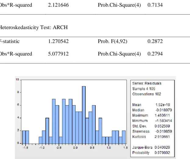
(Breusch-Godfrey Serial Correlation LM Test and ARCH Test)

Breusch-Godfrey Serial Correlation LM Test:

F-statistic 0.488573 Prob. F(4,92) 0.7441

Obs*R-squared 2.121646 Prob.Chi-Square(4) 0.7134

Heteroskedasticity Test: ARCH

F-statistic 1.270542 Prob. F(4,92) 0.2872

Obs*R-squared 5.077912 Prob.Chi-Square(4) 0.2794

FIGURE 5 – Jarque-Bera residual test

The null hypothesis of no serial correlation is not rejected by the Breusch-Godfrey LM test, at a 5% significance level. The null hypothesis of no heteroskedasticity is also not rejected in the ARCH test for the same significance level. The Jarque-Bera test provides statistical evidence that the residuals follow a normal distribution.

Figure 6 shows the impulse response of US Dollar Index to a one unit shock in Brent Crude Oil price.

25

FIGURE 6: Response of US Dollar Index to a shock in Brent Crude Oil price

As stated by some authors mentioned previously in the literature review, an increase in Brent Crude Oil price implies a decrease in US Dollar Index.

5.2. Relationship between Brent Crude Oil price, the US Dollar Index and agricultural commodities prices

Do Brent Crude Oil prices, US Dollar Index and the price of agricultural commodities go together in the long-run or, in other words, do they reveal a long-term relationship, in spite of its non-stationary behavior in level? To ask this question we run the Johansen test, using, each time, one of the agricultural commodities with the pair Brent Crude Oil-US Dollar Index.

Johansen’ tests for cointegration were preceded by the determination of the optimal lag length and the optimal model to use, chosen among the five models of VECM. The results of the Johansen’s trace test for cointegration are reported in Table VIII and the complete results of trace tests are in Tables XV to XXI.

26

TABLE VIII Johansen’s trace test

(Brent Crude Oil price, US Dollar Index and each agricultural commodity)

Model 2 5%* Coffee Cotton r=2 9,16 2,44 3,36 r=1 20,26 16,00 16,14 r=0 35,19 40,32 42,60 Model 4

5% * Cocoa Sugar Soybean Wheat Corn r=2 12,52 6,96 5,36 9,55 7,30 5,38 r=1 25,87 20,70 17,64 21,71 15,56 13,54 r=0 42,92 46,74 53,44 64,80 46,98 46,10

*Critical Values

In all cases, the trace statistic indicates a cointegration rank of r = 1, given a 5% significance level. So we can conclude that there is one cointegrating vector between Brent Crude Oil price, US Dollar Index and each one of the other commodities, which reflects the long-run relationship among those three variables.

The next step is to create VEC models which allow us to quantify the short and long-run correlations. Lag 2 was determined by Akaike Information Criteria as being the optimal lag length to use in all the models. ΔCommodityt1and ΔCommodityt2represent lag 1

27

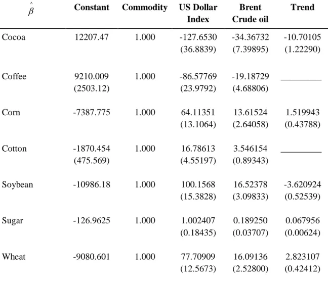
The cointegrating vectors

^

 , normalized to the agricultural commodity, are in Table IX.

The adjustment coefficients

^

 and the equations that represent the short run relationship among the variables are in Table X.

TABLE IX Cointegrating vectors

^

 Constant Commodity US Dollar Index Brent Crude oil Trend Cocoa 12207.47 1.000 -127.6530 (36.8839) -34.36732 (7.39895) -10.70105 (1.22290) Coffee 9210.009 (2503.12) 1.000 -86.57769 (23.9792) -19.18729 (4.68806) _________ Corn -7387.775 1.000 64.11351 (13.1064) 13.61524 (2.64058) 1.519943 (0.43788) Cotton -1870.454 (475.569) 1.000 16.78613 (4.55197) 3.546154 (0.89343) _________ Soybean -10986.18 1.000 100.1568 (15.3828) 16.52378 (3.09833) -3.620924 (0.52539) Sugar -126.9625 1.000 1.002407 (0.18435) 0.189250 (0.03707) 0.067956 (0.00624) Wheat -9080.601 1.000 77.70909 (12.5673) 16.09136 (2.52800) 2.823107 (0.42412)

28

TABLE X

Short Run Parameter Estimates

Variable/Equation

ΔCocoa ΔCoffee ΔCorn ΔCotton ΔSoybean ΔSugar ΔWheat

^  -0.178** (0.049) -0.009 (0.008) -0.062** (0.025) -0.008 (0.013) -0.129** (0.040) -0.149** (0.058) -0.019 (0.034) Constant 10.642 (7.759) _____ -1.867 (1.628) _____ 4.128 (3.584) -0.046 (0.058) -2.808 (2.079) ΔCommodity.t1 -0.085 (0.096) 0.190* (0.103) -0.040 (0.100) -0.042 (0.101) 0.042 (0.098) 0.058 (0.105) 0.058 (0.105) ΔCommodityt₂ -0.122 (0.096) -0.018 (0.105) -0.022 (0.099) -0.080 (0.105) 0.145 (0.098) 0.004 (0.105) 0.029 (0.506) ΔUSD_Indext1 -2.126 (10.591) 0.040 (1.185) 3.121 (2.179) 0.094 (0.354) 12.062** (4.834) -0.027 (0.075) -2.171 (2.894) ΔUSD_Indext2 -7.809 (10.276) 1.197 (1.150) 2.664 (2.157) -0.222 (0.342) 8.879* (4.777) -0.023 (0.073) 1.743 (2.807) ΔBrentC.Oil t1 -5.360* (3.038) 0.221 (0.359) 0.740 (0.656) 0.050 (0.107) 2.722* (1.519) 0.028 (0.024) 0.800 (0.848) ΔBrentC.Oil t₂ 2.296 (3.136) -0.084 (0.367) 0.843 (0.673) -0.037 (0.108) 4.530** (1.552) 0.041* (0.023) -0.424 (0.884)

** Denotes significance at the 5% level * Denotes significance at the 10% level

Some conclusions can be taken about the significance of the model:

All coefficients of Δwheat and Δcotton model are not statistically significant at a 10% level. Therefore, both models must be read with extremely caution.

29

In Δcocoa, Δcorn, Δsoybean and Δsugar models, the adjustment coefficient alpha (

^  ) is significant at a 5% or lower level. The higher values of that coefficient in ΔCocoa, Δsugar and Δsoybean reflects a higher speed of adjustment to equilibrium than in ΔCorn. ΔSoybean is the model with the most statistically significant coefficients.

As it was previously referred, this model is based in the assumption that residuals follow a white noise process. So we need to check if the residuals are normally distributed, with zero mean, with no serial correlation, and show no arch effect.

Table XI reports the results of these tests.

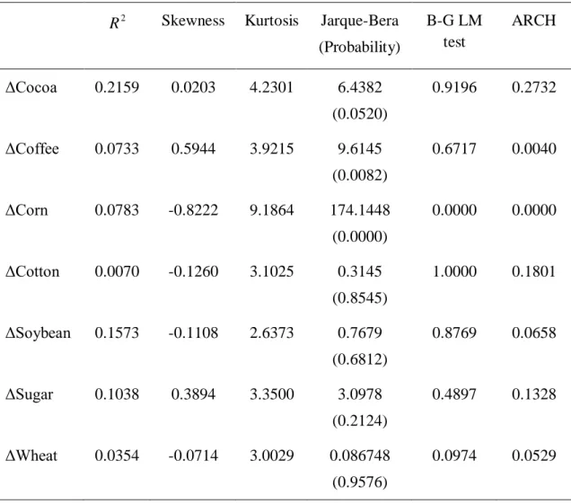
TABLE XI

Tests and Residual Diagnostics

2

R Skewness Kurtosis Jarque-Bera

(Probability) B-G LM test ARCH ΔCocoa 0.2159 0.0203 4.2301 6.4382 (0.0520) 0.9196 0.2732 ΔCoffee 0.0733 0.5944 3.9215 9.6145 (0.0082) 0.6717 0.0040 ΔCorn 0.0783 -0.8222 9.1864 174.1448 (0.0000) 0.0000 0.0000 ΔCotton 0.0070 -0.1260 3.1025 0.3145 (0.8545) 1.0000 0.1801 ΔSoybean 0.1573 -0.1108 2.6373 0.7679 (0.6812) 0.8769 0.0658 ΔSugar 0.1038 0.3894 3.3500 3.0978 (0.2124) 0.4897 0.1328 ΔWheat 0.0354 -0.0714 3.0029 0.086748 (0.9576) 0.0974 0.0529

30

According to the tests, we can’t reject the null hypotheses that ΔCorn and ΔCoffee models exhibit heterokedasticity in residuals for a 5% significance level. ΔCorn fails too in LM test and Jarque-Bera test, so we can’t reject the null hypotheses of a non normal distribution of the residuals and the existence of no serial correlation. ΔCoffee fails too in Jarque-Bera test. According to the results contained in Tables X and XI, we pursuit with the study of Soybean, Cocoa and Sugar models as being the best fitted models obtained in this study.

The relatively low values of R squared were already expected due to the small number of the explanatory variables. We may not forget that we are dealing with futures prices on agricultural commodities, which are highly dependent on weather conditions. Natural disasters or periods of dry in the main export countries causes extremely volatility in prices which are not a direct cause of changes in the Brent Crude Oil prices and the US Dollar Index.

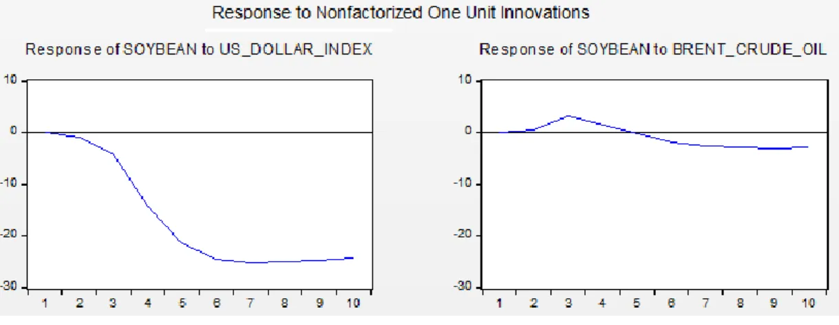
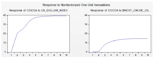
Figures 7, 8 and 9 show respectively the impulse response of Soybean, Cocoa and Sugar to a one unit shock in US Dollar Index and Brent Crude Oil prices.

FIGURE 7: Response of Soybean prices to a shock in US Dollar Index and in Brent Crude Oil price

31

FIGURE 8: Response of Cocoa prices to a shock in US Dollar Index and in Brent Crude Oil price

FIGURE 9: Response of Sugar prices to a shock in US Dollar Index and in Brent Crude Oil price

We verify that Sugar and Soybean respond positively to an increase of one unit in US Dollar Index and sugar tends to decrease its price. The response of Soybean to a unit shock in US Dollar Index has two distinguished periods: first Soybean price increases and then (around period t+5) decreases to lower values than the pre-shock level. In the other hand, Sugar remains relatively stable to a unit shock in Brent Crude Oil price.

32

6. Summary and conclusions

With the recent unusual volatility in the prices of some agricultural commodities and the Brent Crude Oil plumbing being often blamed for that, this dissertation aimed to test the strength of this correlation and to what extent speculators can use it as a benchmark. The dollar strength, being quantified as the US Dollar Index, was also used as an independent variable highlighting the possible direct impact that Forex markets can cause to these variables which are all quoted in US Dollars on ICE (Intercontinental Exchange, inc.).

First, we started by studying the correlation between the Brent Crude Oil prices and the US Dollar Index. We found a cointegrating vector between these two variables (which revealed the inverse relationship between them) and, applying the Granger Causality test, we found that a change in Brent Crude Oil prices causes a change in US Dollar Index.

A regard over the plot of both time series also highlights this relationship. The recent plunge of Brent Crude Oil prices due to Iran´s increasingly oil production after having its sanctions lifted, and the slowdown of China´s manufacturing were followed by an enormous spike in the US Dollar Index.

The next step was to study the cointegrating relations between Brent Crude Oil prices, the US Dollar Index and each one of the selected agricultural commodities.

Through the application of the ADF and Johansen trace tests we concluded that all variables are stationary of order one and there is one cointegrating vector between all the three variables.

Next, we built vector error correction models and conducted its analysis and the study of residuals.

33

Low statistical significance was found for all coefficients of Wheat and Cotton. A feature which may indicate the low dependence of petroleum based inputs in these crops and a stable demand and supply of these commodities independently of Forex markets. For Cocoa, Soybean, Sugar and Corn we have statistically significant coefficients of adjustment (alpha). The low value of alpha for Corn indicates a slow retrace of this commodity to equilibrium after a shock. The ARCH test made for this variable also indicates that we can´t reject the hypothesis of heteroskedasticity in its residuals for a 5% significance level.

The Soybean model was the one with the most statistically significant coefficients. A feature certainly related with the increasingly use of Soybean in the production of biofuel.

On the other hand, one of the most unexpected conclusions of this dissertation was the lack of correlation between Corn prices and the prices of Brent Crude Oil.

The use of Corn for the production of ethanol, which can be used as a substitute for both crude oil and gasoline, would expectedly create a link between these variables as pointed out by Natalenov et al (2013).

Nevertheless, this type of research must be carefully interpreted, since correlations might appear in different periods of time as was already proven by different studies. One thing we can be sure: Brent Crude Oil and the strength of the US Dollar do play a role in the price variation of agricultural commodities which should not be forgotten by both, speculators and agricultural companies who wish to hedge their exposure.

34

7. References

Abbott P., Hunt C & Tyner, W.E. (2008) What’s Driving Food Prices? Farm Foundation Issue Report, July 2008

Akaike, H. (1973). Information Theory and an Extension of the Maxcimum Likehood Principle. In: B.N Petrov and F.Csáki. 2nd International Symposium of Information

Kiadó, Budapest: 267-281

Asteriou, D. & Hale S. (2007). Applied Econometrics, a Modern Approach, Revised Edition, New York: Palgrave MacMillan.

Bação, P. (2000). Identificação de Vectores de Cointegração: Análise de Alguns Exemplos. Grupo de Estudos Monetários e Financeiros (GEMF). Universidade de Coimbra.

Campiche, J., Bryant,H., Richardson, J.W. & Outlaw, J.L. (2007). Examining the Evolving Correspondence Between Petroleum Prices and Agricultural Commodity Prices. Agricultural and Food Policy Center, Texas University.

URL http://ageconsearch.umn.edu/bitstream/9881/1/sp07ca04.pdf Dwyer, G (2014). The Johansen Tests for Cointegration.

URLhttp://www.jerrydwyer.com/pdf/Clemson/Cointegration.pdf

Futures Industry Associaciation (FIA), 2014. Annual Global Futures and Options Volume. URL: http://fimag.fia.org

Golub, S.S. (1983), Oil Prices and Exchange Rates. The Economic Journal 93, 576–593. Granger, W (1969). Investigating Causal Relations by Econometric Models and

Cross-Spectral Methods. Econometrica, 37: 424-438

35

Harri A., Nalley N. & Hudso D. (2009). The Relationship Between Oil, Exchange Rates, and Commodity Prices. Journal of Agricultural and Apllied Economics, 41,2 (August 2009): 501-510.

Margarido, M (2004). Teste de Cointegração de Johansen utilizando o SAS. Instituto de Economia Agrícola, São Paulo, v. 51, n. 1, (jan./jun. 2004): 87-101.

Murphy, J. (1999). Technical Analysis of the Financial Markets. Tenth Edition. New York Institute of Finance. New York.

Natalenov, V., McKenzie, A. & Huylenbroek, G. H. (2013). Crude Oil – Corn – Ethanol – Nexus: A Contextual Approach. Energy Policy, (December 2013) 63, 504-513

Nazlioglu, S., Erden, C. & Soytas, U. (2012). Volatility Spillover Between Oil and Agricultural Commodities Markets. Energy Economics (March 2013). URL http://dx.doi.org/10.1016/j.eneco.2012.11.009

Novotny, F. (2012). The Link Between the Brent Crude Oil Price and the US Dollar Exchange Rate. Prague Economic Papers, 2, 220-232.

Pfaff, Bernhard(2008). VAR, SVAR and SVEC models: Implementation Within R Package Vars. URLhttps://cran.r-project.org/web/packages/vars/vignettes/vars.pdf Rosa, F & Vasciaves M. (2012). Agri-Commodity Price Dynamics: The Relationship

Between Oil and Agricultural Market. Department of Food Science – University of Udine Italy.

Tsay, R (2005). Analysis of Finantial Time Series, Second Edition, Chicago: Wiley Interscience.

Zhang, Y (2013). The Links Between the Price of Oil and the Value of US Dollar. International Journal of Energy Economics and Policy. Vol 3, nº4: 341-351

36

8. Appendix

37

TABLE XII

Optimal Lag Length Selection

VAR Lag Order Selection Criteria

Endogenous Variables: ΔUS Dollar Index; ΔBrent Crude Oil Exogenous variables. C

Sample: 1 104

Included observations: 96

Lag LogL LR FPE AIC SC HQ

0 -334.6701 NA 3.812208 7.013961 7.067385* 7.035556* 1 -331.9596 5.251681 3.916159 7.040825 7.201097 7.105609 2 -329.5311 4.604002 4.047095 7.073565 7.340684 7.181539 3 -326.5349 5.555487 4.133983 7.094477 7.468444 7.245641 4 -321.0074 10.01864 4.006844 7.062653 7.543469 7.257007 5 -313.7193 12.90592* 3.744995 6.994152* 7.581816 7.231696 6 -312.6928 1.775068 3.989609 7.056099 7.750610 7.336832 7 -309.7278 5.003447 4.083971 7.077662 7.879021 7.401584 8 -305.1986 7.454203 4.048841 7.066638 7.974845 7.433750

* indicates the lag order selected by each criterion

LR: sequential modified LR test statistic (each test at a 5% level) FPE: Final Prediction Error

AIC: Akaike Information Criterion SC: Schwarz Information Criterion HQ: Hannan-Quinn Information Criterion

38

Table XIII

Choosing appropriate model for VECM on Brent Crude Oil price and US Dollar Index, using AIC

Sample: 1 105

Included observations: 102

Series: Brent Crude Oil; US Dollar Index Lags interval: 1 to 2

Selected Number of Cointegrating Relations by Model*

Data Trend: None None Linear Linear Quadratic

Test Type No intercept

No Trent Intercept No Trend Intercept No Trend Intercept Trend Intercept Trend Trace 0 1 1 1 1 Max-Eig 0 1 1 1 1

* For a 0.05 critical level based on Mackinnon-Michelis (1999)

Information Criteria by Rank and Model

Data Trend: None None Linear Linear Quadratic

Rank or No. of CEs No intercept No Trent Intercept No Trend Intercept No Trend Intercept Trend Intercept Trend Log Likelihood by Rank (rows) and Model (columns)

0 -355.4618 -355.4618 -354.1336 -354.1336 -348.6842

1 -352.1384 -343.9428 -342.8802 -342.7444 -339.0490

2 -351.7681 -342.2848 -342.2848 -339.0415 -339.0415

Akaike Information Criteria by Rank (rows) and Model (columns)

0 7.126702 7.126702 7.139875 7.139875 7.072239

1 7.139968 6.998878 6.997651 7.014596 6.961744

2 7.211138 7.064408 7.064408 7.040029 7.040029

Schwarz Criteria by Rank (rows) and Model (columns)

0 7.332582* 7.332582* 7.397225 7.397225 7.381060

1 7.448789 7.333434 7.357942 7.400621 7.373505

39

TABLE XIV

Statistics from VECM (Brent Crude Oil – US Dollar Index)

Dependent Variable: ΔUS Dollar Index

Method: Least Squares (Gauss-Newton/ Marquardt steps) Sample (adjusted): 4 105

Included observations: 102 after adjustments

ΔUS Dollar Index = C(1)*(US Dollar Index(-1) + 0.213789219932*Brent Crude

Oil(-1) – 106.798130314) + C(2)*ΔUS Dollar Index(-Oil(-1) + C(3)*ΔUS Dollar Index(-2) + C(4)*ΔBrent Crude Oil(-1) + C(5)*ΔBrent Crude Oil(-2) + C(6)

Coefficient Std. Error t-statistic Prob.

C(1) -0.347140 0.074029 -4.689233 0.0000 C(2) 0.078188 0.095116 0.822025 0.4131 C(3) 0.007491 0.093250 0.080333 0.9361 C(4) 0.016668 0.028125 0.592639 0.5548 C(5) 0.010264 0.028999 0.353952 0.7242 C(6) 0.122964 0.069981 1.757100 0.0821

R-squared 0.237203 Mean dependent var 0.116725

Adjusted R-squared 0.197474 S.D. dependent var 0.747175

S.E. of regression 0.669348 Akaike Information Criterion 2.091996

Sum squared resid 43.01052 Schwarz criterion 2.246406

Log likelihood -100.6918 Hannan-Quinn Criterion 2.154522

F-statistic 5.970516 Durbin-Watson stat 1.992487

40

TABLE XV

Johansen Test Results - Corn, Brent Crude Oil, US Dollar Index (model 4, lags 2)

Included observations: 102 after adjustments

Trend assumption: Linear deterministic trend (restricted) Series: Corn; Brent Crude Oil; US Dollar Index

Lags interval (first differences): 1 to 2

Unrestricted Cointegration Rank Test (Trace)

Hypothesized No. of CE(s)

Eigenvalue Trace Statistic 0.05

Critical Value Prob. None 0.273253 46.10040 42.91525 0.0232 At most 1 0.076893 13.54438 25.87211 0.6949 At most 2 0.051409 5.383351 12.51798 0.5423 TABLE XVI

Johansen Test Results - Sugar, Brent Crude Oil, US Dollar Index (model 4, lags 2)

Included observations: 102 after adjustments

Trend assumption: Linear deterministic trend (restricted) Series: Sugar; Brent Crude Oil; US Dollar Index

Lags interval (first differences): 1 to 2

Unrestricted Cointegration Rank Test (Trace)

Hypothesized No. of CE(s)

Eigenvalue Trace Statistic 0.05

Critical Value

Prob.

None 0.296016 53.43801 42.91525 0.0033

At most 1 0.113410 17.63603 25.87211 0.3689

41

TABLE XVII

Johansen Test Results - Coffee, Brent Crude Oil, US Dollar Index (model 2, lags 2)

Included observations: 102 after adjustments

Trend assumption: Linear deterministic trend (restricted) Series: Coffee; Brent Crude Oil; US Dollar Index

Lags interval (first differences): 1 to 2

Unrestricted Cointegration Rank Test (Trace)

Hypothesized No. of CE(s)

Eigenvalue Trace Statistic 0.05

Critical Value Prob. None 0.212152 40.32248 35.19275 0.0128 At most 1 0.124511 16.00060 20.26184 0.1744 At most 2 0.023613 2.437398 9.164546 0.6900 TABLE XVIII

Johansen Test Results - Cocoa, Brent Crude Oil, US Dollar Index (model 4, lags 2)

Included observations: 102 after adjustments

Trend assumption: Linear deterministic trend (restricted) Series: Cocoa; Brent Crude Oil; US Dollar Index

Lags interval (first differences): 1 to 2

Unrestricted Cointegration Rank Test (Trace)

Hypothesized No. of CE(s)

Eigenvalue Trace Statistic 0.05

Critical Value

Prob.

None 0.225293 46.74146 42.91525 0.0198

At most 1 0.126038 20.70391 25.87211 0.1923

42

TABLE XIX

Johansen Test Results - Cotton, Brent Crude Oil, US Dollar Index (model 2, lags 2)

Included observations: 102 after adjustments

Trend assumption: Linear deterministic trend (restricted) Series: Cotton; Brent Crude Oil; US Dollar Index

Lags interval (first differences): 1 to 2

Unrestricted Cointegration Rank Test (Trace)

Hypothesized No. of CE(s)

Eigenvalue Trace Statistic 0.05

Critical Value Prob. None 0.228542 42.60460 35.19275 0.0067 At most 1 0.117711 16.13835 20.26184 0.1680 At most 2 0.032446 3.364344 9.164546 0.5149 TABLE XX

Johansen Test Results - Soybean, Brent Crude Oil, US Dollar Index (model 4, lags 2)

Included observations: 102 after adjustments

Trend assumption: Linear deterministic trend (restricted) Series: Soybean; Brent Crude Oil; US Dollar Index Lags interval (first differences): 1 to 2

Unrestricted Cointegration Rank Test (Trace)

Hypothesized No. of CE(s)

Eigenvalue Trace Statistic 0.05

Critical Value

Prob.

None 0.344551 64.79799 42.91525 0.0001

At most 1 0.112419 21.70967 25.87211 0.1513

43

TABLE XXI

Johansen Test Results - Wheat, Brent Crude Oil, US Dollar Index (model 4, lags 2)

Included observations: 102 after adjustments

Trend assumption: Linear deterministic trend (restricted) Series: Wheat; Brent Crude Oil; US Dollar Index

Lags interval (first differences): 1 to 2

Unrestricted Cointegration Rank Test (Trace)

Hypothesized No. of CE(s)

Eigenvalue Trace Statistic 0.05

Critical Value

Prob.

None 0.265074 46.97554 42.91525 0.0186

At most 1 0.077810 15.56100 25.87211 0.5282