Tomografia passiva costiera (TOMPACO). Inversion results with passive data - phase 3

(1)

CINTAL - Centro de Investiga¸

c˜

ao Tecnol´

ogica do Algarve

Universidade do Algarve

Tomografia Passiva Costiera

(TOMPACO)

Inversion results with passive data - Phase 3

S.M. Jesus and C. Soares

Rep 02/03 - SiPLAB 28/March/2003

University of Algarve tel: +351-289800131

(2)

Work requested by CINTAL

Universidade do Algarve, Campus da Penha, 8005-139 Faro, Portugal

tel: +351-289800131, cintal@ualg.pt, www.ualg.pt/cintal

Laboratory performing SiPLAB - Signal Processing Laboratory

the work Universidade do Algarve, FCT, Campus de Gambelas,

8000 Faro, Portugal

tel: +351-289800949, info@siplab.uceh.ualg.pt, www.fct.ualg.pt/adeec/siplab

Projects TOMPACO - CNR, Italy

Title TOMografia PAssiva COstiera - (Phase 3)

Authors S.M.Jesus and C.Soares

Date March 28, 2003

Reference 02/03 - SiPLAB

Number of pages 31 (thirty one)

Abstract This report shows the acoustic inversion results obtained

on the INTIFANTE’00 data set, Events II, IV, V and VI.

Clearance level UNCLASSIFIED

Distribution list DUNE (1), ENEA (1), IH (1), SiPLAB (1), CINTAL (1)

Total number of copies 5 (five)

(3)

III

Foreword and Acknowledgment

This report presents the acoustic tomography inversion results obtained by CINTAL un-der project TOMPACO, on the INTIFANTE’00 data set. The INTIFANTE’00 sea trial

took place off the Tr´oia Peninsula, near Set´ubal, approximately 50 km south of Lisbon,

Portugal, during the period 9 - 29 October 2000. The institutions responsible for the sea trial are:

• Instituto Hidrogr´afico, Rua das Trinas 49, Lisboa, Portugal.

• CINTAL, Universidade do Algarve, Faro, Portugal. • ISR, Instituto Superior T´ecnico, Lisboa, Portugal. Other institutions involved are:

• Ente Nazionale per l’Energia ed l’Ambiente, La Spezia, It´alia

The INTIFANTE organizers would like to thank: • the crew of the research vessel NRP D. Carlos I

• the NATO SACLANT Undersea Research Centre for lending the acoustic sound source and power amplifier.

(4)

IV

(5)

List of Figures

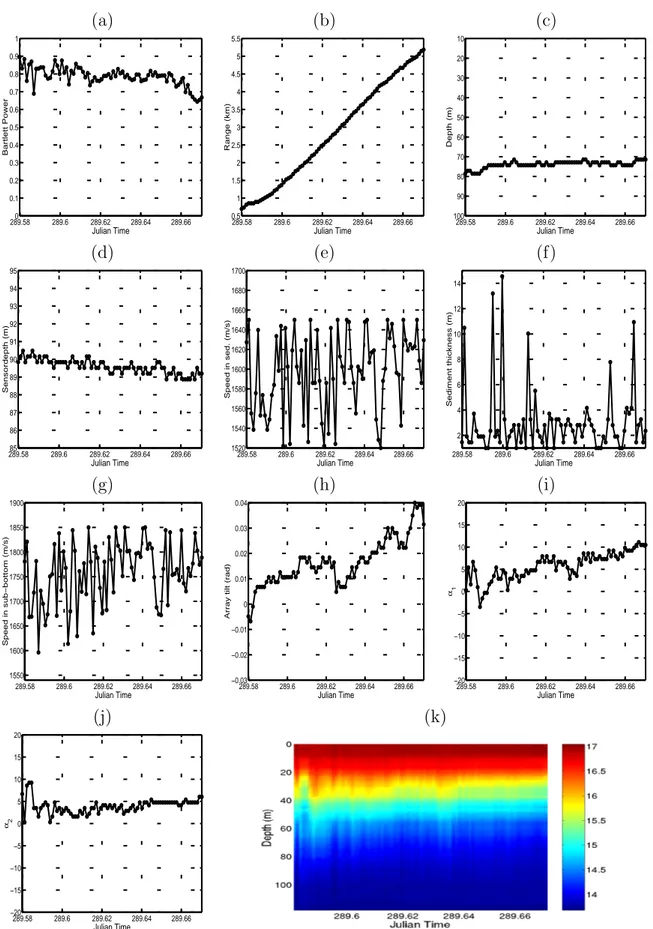
2.1 Focalization results for first part of Event 2: Bartlett power (a), source

range (b), source depth (c), receiver depth (d), sediment compressional speed (e), sediment thickness (f ), sub-bottom compressional speed (g), VLA tilt (h), EOF coefficient 1 (i), EOF coefficient 2 (j) and reconstructed

tem-perature profiles (k). . . 12

2.2 Focalization results for second part of Event 2: cross-frequency Bartlett

power (a), source range [dashed curve is the GPS measured source - VLA range (see footnote)](b), source depth (c), receiver depth (d), VLA tilt (e), EOF coefficient 1 (f ), EOF coefficient 2 (g) and estimated temperature

profiles over time (h). . . 13

2.3 Focalization results for second part of Event 2 with full search: source range

(a), source depth (b), and estimated temperature profiles excluding off-focus estimates (c) and respective reconstructed temperature estimate over time

(d). . . 14

2.4 Tidal prediction during Event 2: tidal height (a) and tidal variation (b). . . 15

2.5 Focalization results for Event 4: Bartlett power (a), source range (b), source

depth (c), receiver depth (d), sediment compressional speed (e), sediment thickness (f ), sub-bottom compressional speed (g), VLA tilt (h), EOF co-efficient 1 (i), EOF coco-efficient 2 (j) and reconstructed temperature profiles

(k). . . 16

2.6 Tidal prediction during Event 4: tidal height (a) and tidal variation (b). . . 17

2.7 Focalization results for Event 5: Bartlett power (a), source range (b), source

depth (c), receiver depth (d), sediment compressional speed (e), sediment thickness (f ), sub-bottom compressional speed (g), VLA tilt (h), EOF co-efficient 1 (i), EOF coco-efficient 2 (j) and reconstructed temperature profiles

(k). . . 18

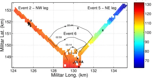
3.1 INTIFANTE’00 sea trial Event 6 and site bathymetry. XBT casts locations

are marked with X and ULVA denotes the VLA location. . . 20

3.2 Event 6: GPS measured ship speed (a) and ship heading (b). . . 20

3.3 Baseline model for ship noise data inversion during Event 6. . . 21

3.4 NRP D. Carlos I ship radiated noise received on hydrophone 8:

(8)

VIII LIST OF FIGURES

3.5 INTIFANTE’00 sea trial, event 6: selected frequency bins for inversion. . . 22

3.6 Focalization results for Event 6: Bartlett power (a), source range (b)[the

dashed line is the GPS measured source-receiver range and arrows indi-cate sharp turns] , source depth (c), receiver depth (d), VLA tilt (e), EOF

coefficient 1 (f ), EOF coefficient 2 (g) and reconstructed temperature (h). . 24

3.7 INTIFANTE’00 sea trial, event 6, 16 s data window for hydrophone 8

at Julian time 291.125: spectrogram (a) and selected frequency bins for

inversion using the minimum variance criterion (b). . . 25

3.8 Focalization results for Event 6 (second attempt): Bartlett power (a), source

range (b)[the dashed line is the GPS measured source-receiver range] , source depth (c), receiver depth (d), VLA tilt (e), EOF coefficient 1 (f ), EOF coefficient 2 (g) and reconstructed ocean temperature profile over time

(h). . . 26

3.9 INTIFANTE’00 sea trial, event 6: source spectrum estimate over time. . . 27

4.1 INTIFANTE’00 sea trial: temperature profiles estimated with passive

(9)

Chapter 1 Introduction

Passive Acoustic Tomography (PAT) is an acoustic tomography variant where the usual cooperative acoustic source is replaced by a non-cooperative noise source as for example a ship of opportunity. The basic idea behind PAT is to extend the application of acoustic tomography to areas with heavy or regular ship traffic and where it would be impossible, or too costly, to deploy a controlled acoustic source in a permanent basis.

PAT differs from classic active acoustic tomography by the fact that in PAT, the source signal is stochastic with unknown characteristics and uncontroled by the experimenter. There are at least two important implications of the assumptions made under PAT: one is that the emitted signal is possibly fluctuating over time both in strenght and bandwidth, the other is that the sound source’s position is unknown and possibly changing over time. The fact that the source position is unknwon implies that apart from the sound speed profile to be inverted for, the other propagation channel characteristics (e.g. bottom properties, water depth, etc...) are also unknown. An inverse problem where both the input signal and the channel are unknown is termed a blind deconvolution problem, and is common in the fields of wireless communications, geophysics and in all problems where channel identification is required and where the input signal is not known (see Cadzow [1] for an overview). The generally adopted methodology is to use higher-order statistics and (in wireless communications) the ciclostationarity properties of the received signal [2, 3]. Such methods have also been used in underwater acoustics for signals with some degree of non-stationarity [4, 5]. Assuming that the noise sources of opportunity are relatively stationary inputs to the propagation channel it is possible to build a model-based cost function where both the source and the channel properties are unknown variables to be estimated.

Project TOMPACO (TOMografia PAssiva COstiera) was proposed in 1999 by DUNE with the goal of testing the feasibility of the PAT concept. To that aim, CINTAL (a TOMPACO subcontractor) has setup an experiment to acquire real acoustic data to sup-port TOMPACO. That experiment took place in October 2000 under the framework of the INTIFANTE’00 sea trial. An overview of the sea trial can be found in [6, 7] and inter-mediate reports specifically dealing with TOMPACO issues were produced regarding the acquired data set [8] and the inversion results with active data [9]. This third TOMPACO report is intended to analyse the results obtained using ship noise data as input signals (passive data) and draw the final conclusion for the practical feasibility of the proposed methodology.

This report is organized as follows: chapter 2 summarizes the tomographic inversion results obtained on the INTIFANTE’00 data set using, in section 2.1, known sound source

(10)

10 CHAPTER 1. INTRODUCTION

signals over a range-independent area (Event 2) and in section 2.2 with the source navi-gating over a range-dependent area. Chapter 3 deals with new results obtained during Event 6 where the source signal was the research ship NRP D. Carlos I, herself. Final conclusions and perspectives are drawn in chapter 4.

(11)

Chapter 2 Acoustic tomography results

obtained during INTIFANTE’00:

active data

The INTIFANTE’00 sea trial was primarely designed for testing acoustic data inversion techniques aiming at estimating water column properties and source position. A com-plete description of the sea trial can be found in previous TOMPACO reports [8, 9] and in conference Proceedings [7] and therefore will not be repeated here. Part of these results were the object of a plenary invited session during the European Conference on Under-water Acoustics held in Gdansk (Poland) in June 2002 [10]. In order to support the final conclusions drawn at the end of this report a brief overview of the results obtained with active data already reported in [9] are also shown here together with new results obtained on the same data sets.

2.1 Range-independent track: event 2

During Event 2, a series of acoustic 170-600 Hz linear frequency modulated (LFM) sweeps were transmitted over a range independent shallow water waveguide, while the source was towed away from the vertical array location and then held stationary at approximately 5 km range. The results obtained during the first part of this event while the source was moving away from the receiving array are shown in figure 2.1 (also shown in [9]). Here, all the previously made comments apply: the Bartlett power is relatively high throughout the run, source range is nicely and perfectly estimated and all the other parameters are jointly estimated with credible values, including bottom properties. The temperature profiles are modelled by two EOF’s which coefficients show a smooth evolution through time, giving rise to a nicely stratified temperature estimate. At approximately julian time 289.67 the source ship progressively stopped her engines and tried to keep her range of approximately 5.5 km to the VLA. NRP D. Carlos I kept the position for about 15 hours continously transmitting the LFM signals with her source at approximately 80 m depth. For an unknown reason at this point, the usage of a classical broadband Bartlett processor on this data set was unable to correctly localize the sound source and therefore gave no reliable estimates of the environmental data.

(12)

12

CHAPTER 2. ACOUSTIC TOMOGRAPHY RESULTS OBTAINED DURING INTIFANTE’00: ACTIVE DATA

(a) (b) (c) 289.580 289.6 289.62 289.64 289.66 0.1 0.2 0.3 0.4 0.5 0.6 0.7 0.8 0.9 1 Julian Time Bartlett Power 289.58 289.6 289.62 289.64 289.66 0.5 1 1.5 2 2.5 3 3.5 4 4.5 5 5.5 Julian Time Range (km) 289.58 289.6 289.62 289.64 289.66 10 20 30 40 50 60 70 80 90 100 Julian Time Depth (m) (d) (e) (f) 289.5885 289.6 289.62 289.64 289.66 86 87 88 89 90 91 92 93 94 95 Julian Time Sensordepth (m) 289.58 289.6 289.62 289.64 289.66 1520 1540 1560 1580 1600 1620 1640 1660 1680 1700 Julian Time Speed in sed. (m/s) 289.58 289.6 289.62 289.64 289.66 2 4 6 8 10 12 14 Julian Time Sediment thickness (m) (g) (h) (i) 289.58 289.6 289.62 289.64 289.66 1550 1600 1650 1700 1750 1800 1850 1900 Julian Time Speed in sub−bottom (m/s) 289.58 289.6 289.62 289.64 289.66 −0.03 −0.02 −0.01 0 0.01 0.02 0.03 0.04 Julian Time

Array tilt (rad)

289.58 289.6 289.62 289.64 289.66 −20 −15 −10 −5 0 5 10 15 20 Julian Time α1 (j) (k) 289.58 289.6 289.62 289.64 289.66 −20 −15 −10 −5 0 5 10 15 20 Julian Time α2

Figure 2.1: Focalization results for first part of Event 2: Bartlett power (a), source range (b), source depth (c), receiver depth (d), sediment compressional speed (e), sediment thick-ness (f ), sub-bottom compressional speed (g), VLA tilt (h), EOF coefficient 1 (i), EOF coefficient 2 (j) and reconstructed temperature profiles (k).

(13)

2.1. RANGE-INDEPENDENT TRACK: EVENT 2 13

As an alternative a broadband cross-frequency incoherent processor as described in [11] was used instead. The main difference between this processor and the classical Bartlett is that only the off-diagonal cross-frequency terms are used for computing the final objective function while the classical Bartlett uses the auto-frequency terms. The cross-frequency processor was shown to provide the same performance as any coherent processor such as the matched-phase processor proposed by Orris [12] or the normalized coherent proposed by Michalopoulou [13]. (a) (b) (c) 289.9 290 290.1 290.2 290.3 290.4 0 0.2 0.4 0.6 0.8 1 Julian time Bartlett Power 289.9 290 290.1 290.2 290.3 290.4 5 5.2 5.4 5.6 5.8 6 Julian time Range (km) GPS 289.9 290 290.1 290.2 290.3 290.4 0 20 40 60 80 100 Julian time Depth (m) (d) (e) (f) 289.9 290 290.1 290.2 290.3 290.4 88 90 92 94 96 98 Julian time Sensordepth (m) 289.9 290 290.1 290.2 290.3 290.4 −0.04 −0.03 −0.02 −0.01 0 0.01 0.02 0.03 0.04 Julian time

Array tilt (rad)

289.9 290 290.1 290.2 290.3 290.4 −30 −20 −10 0 10 20 30 Julian time α1 (g) (h) 289.9 290 290.1 290.2 290.3 290.4 −30 −20 −10 0 10 20 30 Julian time α2

Figure 2.2: Focalization results for second part of Event 2: cross-frequency Bartlett power (a), source range [dashed curve is the GPS measured source - VLA range (see foot-note)](b), source depth (c), receiver depth (d), VLA tilt (e), EOF coefficient 1 (f ), EOF coefficient 2 (g) and estimated temperature profiles over time (h).

The frequency band used for this data set was formed by 40 frequency bins between 200 and 590 Hz with a 10 Hz spacing. The inversion results using this processor are shown in 2.2 where it was chosen not to invert for the bottom properties since those were

(14)

14

CHAPTER 2. ACOUSTIC TOMOGRAPHY RESULTS OBTAINED DURING INTIFANTE’00: ACTIVE DATA be made regarding these results: 1) the Bartlett power is much lower than usual, which is not strange since now the off-diagonal frequency terms are used which have much lower signal power, 2) source range is oscillating between 5.2 and 6 km with a mean range of 5.6 km perfectly compatible with the VLA - source ship range in the middle part of the

run, as shown by the dashed curve in plot (b)1_{, 3) source depth is relatively stable at}

approximately 78 m depth, apart from the beginning of the run, where the ship was still on the run and slowing down thus the sound source is deepening and at the end of the run (after julian time 290.3) where, for some unknown reason, the estimation process is getting several failures, 4) this pattern is repeated for each parameter estimate including

the EOF’s coefficients α1 and α2and is present in the final temperature estimate on figure

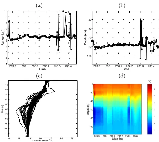
2.2 (h). In order to get a full test whether these estimates were solid and consistent with the data, the search intervals for source position were enlarged to a full length search from 1 to 10 km in range and from 0 to 119 m in depth. The results are shown in figure 2.3. In this case the off-focus estimates are clearly seen to be predominant at the end of the run. Using that information to reject those temperature estimates the reconstructed temperature profiles are shown in plots (c) and (d), where it can be seen that a coherent result could be obtained along the approximately 15 hours of recording.

(a) (b) 289.9 290 290.1 290.2 290.3 290.4 1 2 3 4 5 6 7 8 9 10 Time Range (km) 289.9 290 290.1 290.2 290.3 290.4 20 40 60 80 100 Time Depth (km) (c) (d) 10 12 14 16 18 20 22 10 20 30 40 50 60 70 80 90 100 110 Temperature (o_C) Depth (m)

Figure 2.3: Focalization results for second part of Event 2 with full search: source range (a), source depth (b), and estimated temperature profiles excluding off-focus estimates (c) and respective reconstructed temperature estimate over time (d).

After further investigation on the data for explaining the deviations at the end of the run (after julian time 290.3) it was found that that period does correspond to a reverse of the VLA tilt indicators as mentioned in figure 4.9(c) of report [6] regarding the array 1_{the GPS measured source - VLA range was calibrated with a constant offset of 200 m, that range}

bias might be due to GPS errors, array drift around the mooring and/or acoustic source displacement from the vertical. This bias is consistent with the arrival time peak detection of figure 5.24 of [6].

(15)

2.2. RANGE-DEPENDENT TRACKS: EVENTS 4 AND 5 15

tilt sensor measurements. In fact, at that time the tilt indicators of the shallower portion of the array along the X and Y axis suffer an inversion, denoting a probable change of position of the VLA. That array change is accompanied by a deepening of the whole array by an amount of approximately 1 m, as denoted in the depth sensor recordings of plots (a) and (b) of the same figure (see [6]).

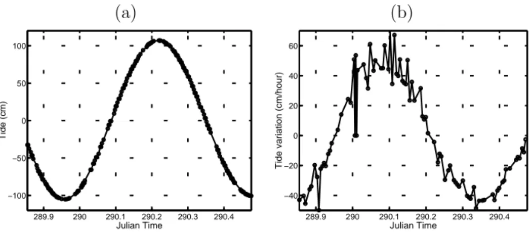
(a) (b) 289.9 290 290.1 290.2 290.3 290.4 −100 −50 0 50 100 Julian Time Tide (cm) 289.9 290 290.1 290.2 290.3 290.4 −40 −20 0 20 40 60 Julian Time

Tide variation (cm/hour)

Figure 2.4: Tidal prediction during Event 2: tidal height (a) and tidal variation (b). Curiously, a simulation of the tide for that day and location (figure 2.4) shows that high water was reached at julian time 290.2 [plot (a)] and is starting to decrease, reaching a maximum current forcing (into the low tide direction) just about julian time 290.3, as shown in the tidal variation of plot (b). This effect might have induced relatively drastic movements on the upper part of the VLA [as seen on the depth and tilt sensor recordings - figure 4.9 (a) and (c) of [6]] strongly perturbating the acoustic inversions.

2.2 Range-dependent tracks: events 4 and 5

Although a range-independent propagation environment is a view of the reality that allows nice theoretical and analytical developments, it is, in most cases, only a simplification that does not represent the large majority of the real world situations. In this section the data gathered during events 4 and 5, along the NE leg, when the source was navigating off from the VLA upto about 5 km range (event 4) and then approaching the VLA (event 5), is used to downslope propagate acoustic signals from approximately 70 m water depth to the receiver located in a 120 m water depth area. Events 4 and 5 represent the most interesting yet, most difficult, case that attempts to represent a realistic situation of an unknwon sound source emitting either deterministic or random signals at undetermined range and depth, moving over a range dependent environment. During Event 4 the source was emitting a series of deterministic LFM signals similar to those used during Event 2. The geometry of the event together with other environmental information is described in report [7]. As it can be seen in figure 2.5, the acoustic source could be accurately tracked, both in range and depth, for about two hours over the range dependent track towards shore [plots (b) and (c)]. During that period the Bartlett power indicator reached 0.9 at a range of 1 km and slowly went down to 0.6 when it suddenly was lost, a little time after julian time 290.8. During that period sensor depth was estimated at credible values between 90 and 91 m, bottom parameters were quite random as expected, array tilt oscillated between -0.01 and 0.025 radians while the EOF coefficients showed credible and stable values. After julian time 290.8 all the inversion process was clearly lost to a very high

(16)

16

(a) (b) (c) 290.74290.76290.78 290.8 290.82290.84290.86290.88 290.9 0 0.1 0.2 0.3 0.4 0.5 0.6 0.7 0.8 0.9 1 Julian Time Bartlett Power 290.74290.76290.78 290.8 290.82290.84290.86290.88 290.9 0.5 1 1.5 2 2.5 3 3.5 4 4.5 5 5.5 6 Julian Time Range (km) 290.74290.76290.78 290.8 290.82290.84290.86290.88 290.9 10 20 30 40 50 60 70 80 90 100 Julian Time Depth (m) (d) (e) (f) 290.74290.76290.78 290.8 290.82290.84290.86290.88 290.9 85 86 87 88 89 90 91 92 93 94 95 Julian Time Sensordepth (m) 290.74290.76290.78 290.8 290.82290.84290.86290.88 290.9 1520 1540 1560 1580 1600 1620 1640 1660 1680 1700 Julian Time Speed in sed. (m/s) 290.74290.76290.78 290.8 290.82290.84290.86290.88 290.9 2 4 6 8 10 12 14 Julian Time Sediment thickness (m) (g) (h) (i) 290.74290.76290.78 290.8 290.82290.84290.86290.88 290.9 1550 1600 1650 1700 1750 1800 1850 1900 Julian Time Speed in sub−bottom (m/s) 290.74290.76290.78 290.8 290.82290.84290.86290.88 290.9 −0.03 −0.02 −0.01 0 0.01 0.02 0.03 Julian Time

Array tilt (rad)

290.74290.76290.78 290.8 290.82290.84290.86290.88 290.9 −20 −15 −10 −5 0 5 10 15 20 Julian Time α1 (j) (k) 290.74290.76290.78 290.8 290.82290.84290.86290.88 290.9 −20 −15 −10 −5 0 5 10 15 20 Julian Time α2

Figure 2.5: Focalization results for Event 4: Bartlett power (a), source range (b), source depth (c), receiver depth (d), sediment compressional speed (e), sediment thickness (f ), sub-bottom compressional speed (g), VLA tilt (h), EOF coefficient 1 (i), EOF coefficient 2 (j) and reconstructed temperature profiles (k).

(17)

2.2. RANGE-DEPENDENT TRACKS: EVENTS 4 AND 5 17

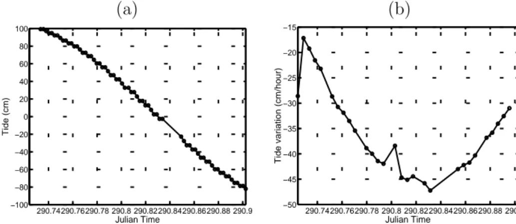
strongly oscillating range and depth estimates as well as most of the other parameters, that some went to the search bounds (EOF coefficients). This situations gave rise to a reconstructed temperature profile that clearly shows two zones: one with believable values before time 290.8 and the other with a very narrow thermocline after that time [plot (k)]. As seen before, coincidence or not, julian time 290.8 does match nearly with the mid tide and the strongest tidal flow (45 cm/hour) at the VLA location as seen in figure 2.6 plots (a) and (b), respectively. Although that might not be the (only) cause of the loss of the inversion process it is interesting to note that, as in event 2, the estimation process proceeds fairly well during source tow and is poor during fixed position source recordings.

(a) (b) 290.74290.76290.78 290.8 290.82290.84290.86290.88 290.9 −100 −80 −60 −40 −20 0 20 40 60 80 100 Julian Time Tide (cm) 290.74290.76290.78 290.8 290.82290.84290.86290.88 290.9 −50 −45 −40 −35 −30 −25 −20 −15 Julian Time

Tide variation (cm/hour)

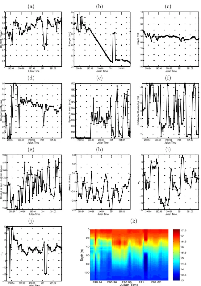
Figure 2.6: Tidal prediction during Event 4: tidal height (a) and tidal variation (b). During Event 5 the source was emitting a pseudo-random noise (PRN) sequence in the band 100 - 2200 Hz, supposed unknown at the receiver. In practice the useful band of the PRN signals is approximately 150 to 1000 Hz due to the acoustic source frequency response. The inversion results are shown in figure 2.7. This run is a good example on how the three indicators - source range, source depth and Bartlett power - can be used to validate environmental model estimates. At the beginning of the run, until julian time 290.96, the Bartlett power varies between 0.4 and 0.8, source range changes rapidly and most of the other parameters have highly variable values and some are on, or near, the bounds of their search intervals. So in these initial period, temperature estimates [plot (k)] can not be considered as valid. At julian time 290.96, source range suddenly picks up at 4 km range and steadly follows the approaching of the source to the VLA up to time 291 at about 2 km source range. During that interval most of the parameters, but the EOF coefficient 1, follow stable values well within their respective intervals and are therefore mostly credible. The first EOF coefficient suffers a strong, and to date unexplained, change at 290.98 right in the midlle of that smooth path. After julian time 291, when the source has reached the closest point of approach to the VLA, the “focus” is again suddenly lost with strong variations on all parameters: drop of the Bartlett power from 0.8 to 0.3, a sudden range variation from 1 to 3.5 km and a drop of 10 m on source depth. It was found that julian time 291 coincides with the low-tide change producing a 1.5 m rise on the array accompained of strong variations on array tilt, as measured on the depth sensors and tiltmeters on the VLA [see figure 4.9 plots (a), (b) and (c) of report [9]]. The model regains “focus” after 15 min with smooth parameter estimates and high Bartlett power values. Among all obtained values within validated intervals, source range and depth were clearly in agreement with the expected values, sound speed in the sediment and bottom are reasonably well estimated to have expected mean values of 1580 and 1700 m/s respectively, with a higher uncertainty in the later, and finally array depth and array tilt are in good agreement with the pressure and tilt sensors colocated with the VLA. After focalization the water temperature was reconstructed - plot (k) - showing a

(18)

18

(a) (b) (c) 290.94 290.96 290.98 291 291.02 0 0.1 0.2 0.3 0.4 0.5 0.6 0.7 0.8 0.9 1 Julian Time Bartlett Power 290.94 290.96 290.98 291 291.02 0.5 1 1.5 2 2.5 3 3.5 4 4.5 5 5.5 Julian Time Range (km) 290.94 290.96 290.98 291 291.02 10 20 30 40 50 60 70 80 90 100 Julian Time Depth (m) (d) (e) (f) 290.94 290.96 290.98 291 291.02 85 86 87 88 89 90 91 92 93 94 95 Julian Time Sensordepth (m) 290.94 290.96 290.98 291 291.02 1520 1540 1560 1580 1600 1620 1640 1660 1680 1700 Julian Time Speed in sed. (m/s) 290.94 290.96 290.98 291 291.02 2 4 6 8 10 12 14 Julian Time Sediment thickness (m) (g) (h) (i) 290.94 290.96 290.98 291 291.02 1550 1600 1650 1700 1750 1800 1850 1900 Julian Time Speed in sub−bottom (m/s) 290.94 290.96 290.98 291 291.02 −0.03 −0.02 −0.01 0 0.01 0.02 0.03 Julian Time

Array tilt (rad)

290.94 290.96 290.98 291 291.02 −20 −15 −10 −5 0 5 10 15 20 Julian Time α1 (j) (k) 290.94 290.96 290.98 291 291.02 −20 −15 −10 −5 0 5 10 15 20 Julian Time α2

Figure 2.7: Focalization results for Event 5: Bartlett power (a), source range (b), source depth (c), receiver depth (d), sediment compressional speed (e), sediment thickness (f ), sub-bottom compressional speed (g), VLA tilt (h), EOF coefficient 1 (i), EOF coefficient 2 (j) and reconstructed temperature profiles (k).

(19)

Chapter 3 Acoustic tomography results

obtained during INTIFANTE’00:

passive data

The real challenge comes when adressing the problem of tomography inversion using ship noise data, i.e., a real unknown and stochastic source signal at unknown location and moving along a poorly known environment. This chapter addresses this problem using as example the data gathered during event 6, when the acoustic source was replaced by the NRP D. Carlos I herself as noise signal generator for tomographic inversion purposes. Some of the results shown here have already been part of a presentation at the Acoustic Variability Conference held in Lerici (Italy), in September 2002 [14].

3.1 Ship-noise track: event 6

During Event 6 the acoustic source was recovered and only the NRP D. Carlos I self noise was used as input signal for tomographic inversion. The research vessel NRP D. Carlos I is a 2800 ton relatively recent ship (1989) which primary purpose was acoustic surveillance when it served under the US flag. She has an overall length of 68 m and a beam of 13 m. Her main propulsion system is formed by two diesel-electric engines developing 800 HP attaining a maximum speed of 11 kn. According to her characteristics NRP D. Carlos I can be considered as an acoustically quite ship. Hence, her use for the purpose of passive tomography under TOMPACO can be considered as providing conservative results when compared with full length cargo ships or tankers travelling at cruising speed. In order to maximize the probabilities of successful inversion and get close to the cruising speeds of “normal” ship traffic, NRP D. Carlos was set to steem at her full speed along a triple bow-shaped pattern as shown in figure 3.1. Ship’s speed and heading during Event 6, as obtained from GPS, is shown in figure 3.2, plots (a) and (b), respectively. It can be seen that NRP D. Carlos I mean speed was about 9 kn with several abrupt drops to 7 kn during the ship sharp turns along the triple bow trajectory.

(20)

20

CHAPTER 3. ACOUSTIC TOMOGRAPHY RESULTS OBTAINED DURING INTIFANTE’00: PASSIVE DATA

Depth (m) 70 80 90 100 110 120 130 124 126 128 130 132 134 149 150 151 152 153 x Event 5 − NE leg x x x ULVA Militar Long. (km) 02:14 02:44 03:14 Event 6 02:59 x x x xx x x Event 2 − NW leg Militar Lat. (km)

Figure 3.1: INTIFANTE’00 sea trial Event 6 and site bathymetry. XBT casts locations are marked with X and ULVA denotes the VLA location.

291.090 291.1 291.11 291.12 291.13 291.14 291.15 291.16 2 4 6 8 10 12 14 Ship speed (kn) (a) 291.090 291.1 291.11 291.12 291.13 291.14 291.15 291.16 100 200 300 400 Bearing (deg) Julian date (b)

Figure 3.2: Event 6: GPS measured ship speed (a) and ship heading (b).

3.1.1 Environmental model

During this test several difficulties are added to the problem, when compared to the previ-ously analized data set obtained in events 2,4 and 5: i) the source is fastly moving, ii) the environment is range dependent and iii) the source signal is ship noise with unknown and presumably time-varying characteristics. On top of those difficulties the actual processing adds also a further problem which is that it is not possible to decide during the processing to switch between a range-independent and a range-dependent environmental models. In principle, a range-dependent model should also hold on the range-independent case, al-lowing water depth at the source end to change along the data inversion. The problem in practice is that due to the well known problem of source range vs. water depth ambigu-ity, it is impossible, or at least extremely difficult to simultaneously estimate source range and water depth. In this analysis it was decided to use a range independent model for

(21)

3.1. SHIP-NOISE TRACK: EVENT 6 21

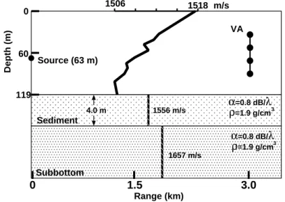
reducing the computation and inversion burden. As it will be seen in the sequel, the usage of a range-independent model, even in a slightly range-dependent environment will add, at some points during the processing, a severe mismatch to the inversion result. There was no extensive oceanographic or geoacoustic survey concerning the area of Event 6, and therefore, geoacoustic inversion estimates obtained during event 2 (above) were used to complete the generic baseline model as pictured in figure 3.3. As in previous analysis a

0 60 119 Depth (m) Range (km) Source (63 m) Sediment Subbottom 0 1.5 3.0 1506 _{1518 m/s} 4.0 m 1556 m/s α =0.8 dB/λ ρ=1.9 g/cm3 α=0.8 dB/λ ρ=1.9 g/cm3 1657 m/s VA

Figure 3.3: Baseline model for ship noise data inversion during Event 6.

two Empirical Orthogonal Function (EOF) based model was used to represent the water column sound speed evolution through time and space, which coefficients are estimated together with the other parameters. The EOF’s are deduced from XBT data taken at locations throughout the experiment site, thus incorporating space and time variability into the EOF expansion (see X signs in figure 3.1). The searched parameters and their respective search intervals are listed in table 3.1.

Table 3.1: Focalization parameters and search intervals: EOF1 (α1), EOF2 (α2), source

range (sr), source depth (sd), receiver depth (rd), VLA tilt (θ) .

Symbol Unit Search int./Steps

α1 m/s -20 20 64 α2 m/s -20 20 64 sr km 0.5 3.5 64 sd m 1 10 32 rd m 85 95 32 θ rad -0.03 0.03 32

3.1.2 Ship radiated noise

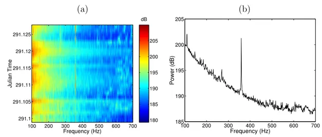
Figure 3.4, shows a time-frequency plot of the signal received on hydrophone 8 at 60 m depth (a), and a mean power spectrum over the whole event (b). There are clearly a few

(22)

22

(a) (b) dB 180 185 190 195 200 205 Frequency (Hz) Julian Time 100 200 300 400 500 600 700 291.1 291.105 291.11 291.115 291.12 291.125 100 200 300 400 500 600 700 185 190 195 200 205 Frequency (Hz) Power (dB)

Figure 3.4: NRP D. Carlos I ship radiated noise received on hydrophone 8: time-frequency plot (a) and mean power spectrum (b).

a strong single tone at 359 Hz. There is also a coloured noise spectra in the band 500 to 700 Hz with, however, a much lower power. As a preliminary analysis, a power spectrum estimator was run on a 8 s sliding time window throughout the whole event duration and the maximum power frequency bins were automatically extracted. Figure 3.5 shows the selected frequency bins that were then used in the inversion procedure.

291.1 291.107 291.114 291.121 291.128 291.135 200 300 359 400 500 600 700 Julian Time Frequency (Hz)

Figure 3.5: INTIFANTE’00 sea trial, event 6: selected frequency bins for inversion.

3.2 Inversion results without source amplitude

esti-mation

The inversion methodology was based on a three step procedure: i) preliminary search of the outstanding frequencies in a given time slot, ii) the usual parameter focalization, based on an incoherent broadband Bartlett processor, a C-SNAP forward acoustic model and a GA based optimization and iii) inversion result validation based on model fitness and coherent source range and depth estimates through time. The inversion results are shown in figure 3.6, from (a) to (g) are individual parameter estimates while plot (h) shows

(23)

3.3. INVERSION RESULTS WITH SOURCE AMPLITUDE ESTIMATION 23

the water column temperature reconstruction based on the EOF linear combination of parameter estimates (f) and (g). Plot (b) shows the estimated source range together with the GPS measured source range (dashed line) and arrows indicate ship turns along the trajectory, with consequent speed drops to 7 kn.

At first glance the results are poor: Bartlett power is low, always below 0.8; source range and depth, which are leading parameters, show highly incoherent values; and finally the reconstructed temperature is too variable for such a small time interval (less than 1h 30min). Looking more in detail, and comparing plot (a) of figure 3.2 with plots (a)-(c) of figure 3.6 the following conclusions can be drawn: i) for time ≤ 291.101 no results can be obtained since the ship is at low speed, Bartlett power is low and parameter estimates are messy; ii) for 291.101 ≤ time ≤ 291.107, ship speed increases steeply to 9 kn, while heading off from the VLA. Range variation is about 4.6 m/s which, may cause a violation of the stationary assumption during the averaging time. Estimates are also messy during this period; iii) at time 291.108, the ship makes a sharp turn, slowing down to 7 kn, and initiates the first bow at an approximate range of 3.2 km and at constant speed of 9kn. At this point the estimation peaks up for a time period between 291.109 to 291.130, i.e. approximately 30 min with a unique exception at 291.119 where there is an estimation loss. That estimation loss curiously corresponds to another sharp turn when the ship heads towards the array between the 3.2 km and the 2.2 km bow. With that exception it can be noticed that range estimates generally coincide to the GPS measurements. There is a slight range error at the begining of the 3.3 km bow (time 291.11) possibly due to range-dependency mismatch which is the strongest at this point (20 m water depth difference between assumed and true). Sensor depth and array tilt show credible values with an interesting behaviour of the later that varies from -0.03 to +0.03 almost linearly and possibly due to a change of the source view angle due to the 45 degree turn along the bow shaped track; iv) at time 291.131 there is another sharp turn towards the VLA with a speed drop and another estimation loss; v) for the remaining few minutes the parameter correct estimation resumes during the closest range bow at 1.2 km from the VLA. As a final comment, it can be added that the reconstructed water temperature suffers from the consecutive losses of estimation that fully coincide with the estimation losses verified in the other curves and are directly related to ship maneuvering and speed drops.

3.3 Inversion results with source amplitude

estima-tion

This second attempt steems from the idea that frequency information and source power may not be being used correctly in this case where the source signal is highly fluctuat-ing both in time and frequency and embedded in noise, causfluctuat-ing difficulties in selectfluctuat-ing frequencies. The broadband inchoerent Bartlett processor has the following form

Pinc(θ) =

PK

k=1|s(ωk)|2hH(ωk, θ)Cyy(ωk)h(ωk, θ)

kH(θ)sk2 , (3-3.1)

where θ is the parameter vector under estimation, h(ωk, θ) is the replica model vector for

all L hydrophones at frequency ωkand for test parameter θ, Cyy(ωk) is the data covariance

matrix at frequency ωk, K is the number of frequencies, H(θ) is a matrix formed with

all replica channel vectors h along the main diagonal and s(ωk) is the source amplitude

at frequency ωk. Equation 3-3.1 is optimum if the noise is spatially uncorrelated and

(24)

24

(a) (b) (c) 291.102 291.11 291.118 291.126 291.134 0 0.2 0.4 0.6 0.8 1 Julian Time Bartlett Power 291.102 291.11 291.118 291.126 291.134 0.5 1 1.5 2 2.5 3 3.5 Julian Time Range (km) 291.102 291.11 291.118 291.126 291.134 1 2 3 4 5 6 7 8 9 10 Julian Time Depth (m) (d) (e) (f) 291.102 291.11 291.118 291.126 291.134 85 90 95 Julian Time Sensordepth (m) 291.102 291.11 291.118 291.126 291.134 −0.03 −0.02 −0.01 0 0.01 0.02 0.03 Julian Time

Array tilt (rad)

291.102 291.11 291.118 291.126 291.134 −20 −15 −10 −5 0 5 10 15 20 Julian Time α1 (g) (h) 291.102 291.11 291.118 291.126 291.134 −20 −15 −10 −5 0 5 10 15 20 Julian Time α2

Figure 3.6: Focalization results for Event 6: Bartlett power (a), source range (b)[the dashed line is the GPS measured source-receiver range and arrows indicate sharp turns] , source depth (c), receiver depth (d), VLA tilt (e), EOF coefficient 1 (f ), EOF coefficient 2 (g) and reconstructed temperature (h).

(25)

often assumed, leading to an equally weighted form of 3-3.1 where |s(ωk)|2 = 1. This

is a suboptimum processor, that is as far from the optimum case as the source power spectrum is non flat and the cross-frequency data correlations are different from zero. It is believed that this is the case for the data set of event 6 where the ship noise spectrum

is highly variable and non flat. The source power estimates ˆs(ωk) where obtained with

a Maximum Likelihood estimator (MLE) conditioned on the environmental parameter θ, of the form ˆ s(ωk) = hH_(ω k, θ)E[y(ωk)] hH_(ω k, θ)h(ωk, θ) . (3-3.2)

The basic idea is to reach a better approximation of the source spectrum in the band used for inversion, thus relaxing the problem of frequency selection: if a low source power frequency is selected at a given time, it will be “correctly” assigned with a low source power estimate. Even in this case, computational limitations lead to the necessity of reducing the frequency sampling, thus another criterion was used to select the spectral components with smaller variance (in a given time frame). This is based on the assumption that the frequency bins with higher variance are more likely to contain only ambient and electronic noise. Thus if the signal variance is estimated by

V (ω, l) = 1 T T X 1 [yl(ω, t) − µy(ω)]2, (3-3.3)

where yl(ω, t) is the received signal on hydrophone k in time window snapshot t at

fre-quency ω, T is the total number of time snapshots and µy(ω) is an estimate of the mean

of yl in the same data window. The frequency components with the lower variance are

those that maximize the functional

v(ω) = _P_L L

l=1V (ω, l)

(3-3.4) where the summation is calculated over the L hydrophones. As an example, applying this criteria to a 16 s duration data window at julian time 291.125 gave the results shown in figure 3.7: spectrogram in (a) and minimum variance selection in (b).

(a) (b) 2000 300 400 500 600 700 0.1 0.2 0.3 0.4 0.5 0.6 0.7 0.8 0.9 1 Frequency (Hz) Likelihood

Figure 3.7: INTIFANTE’00 sea trial, event 6, 16 s data window for hydrophone 8 at Julian time 291.125: spectrogram (a) and selected frequency bins for inversion using the

(26)

26

(a) (b) (c) 291.112 291.117 291.123 291.128 291.134 0 0.2 0.4 0.6 0.8 1 Julian Time Bartlett Power 291.112 291.117 291.123 291.128 291.134 0.5 1 1.5 2 2.5 3 3.5 Julian Time Range (km) GPS 291.112 291.117 291.123 291.128 291.134 1 2 3 4 5 6 7 8 9 10 Julian Time Depth (m) (d) (e) (f) 291.112 291.117 291.123 291.128 291.134 85 90 95 Julian Time Sensordepth (m) 291.112 291.117 291.123 291.128 291.134 −0.03 −0.02 −0.01 0 0.01 0.02 0.03 Julian Time

Array tilt (rad)

291.112 291.117 291.123 291.128 291.134 −20 −15 −10 −5 0 5 10 15 20 Julian Time α1 (g) (h) 291.112 291.117 291.123 291.128 291.134 −20 −15 −10 −5 0 5 10 15 20 Julian Time α2

Figure 3.8: Focalization results for Event 6 (second attempt): Bartlett power (a), source range (b)[the dashed line is the GPS measured source-receiver range] , source depth (c), receiver depth (d), VLA tilt (e), EOF coefficient 1 (f ), EOF coefficient 2 (g) and recon-structed ocean temperature profile over time (h).

(27)

The inversion results using this algorithm and the frequency selection methodology outlined above are given in figure 3.8. When comparing these results with those of figure 3.6 one can note the following differences: i) no estimation drops exist anymore on the source-receiver range estimate at the ship turns [plot (b)], though severe mis-estimates are seen on the other parameters [plots (c) to (g)]; ii) the overall reconstructed temperature profile is much more stable and with a few and clearly indentifiable misses [plot (h)].

As a matter of curiosity 3.9 shows the estimated source spectra using 3-3.2 throughout the inversion procedure of the data set of event 6. This figure shows consistent estimates with the expectations drawn from the previous analysis, i.e., the highest peak is present at a frequency of 359 Hz and this peak disapears at ship turns giving rise to a widely low power spread spectrum over the whole frequency band. This result also justifies the choice of the frequency selection procedure being adopted in this analysis.

200 300 400 500 600 700 291.11 291.115 291.12 291.125 291.13 Julian Time Frequency (Hz) 270 359 719

(28)

Chapter 4 Discussion and final conclusions

OAT is an appealing technique for remote monitoring of the ocean volume. One of the basic principles of OAT is that both source(s) and receiver(s) are under control of the experimentalist, that is, the emitted source signal and the source-receiver geometry is known (with some degree of precision) at all times during the observation window. In passive tomography the control of the source is relaxed, in order to be able to take advan-tage of possible sources of opportunity passing within acoustic range from the receiver(s). Although passive tomography is very appealing for the ease of application, its practical implementation is extremely challenging and its feasibility remains to be proved. To the usual already challenging inverse problem posed by shallow water OAT, there are two difficulties added by passive tomography: one is the fact the source position is unknown to the experimenter and the other is that the emitted signal is random, with an unknown and time-varying power spectrum. In fact, passive OAT becomes a complete indentifica-tion of the propagaindentifica-tion channel without the knowledge of the input signal, both in terms of the emitted signal and source location. Such a problem is known in the literature as “Blind deconvolution”, thus passive OAT is in fact a “Blind Ocean Acoust Tomography” (BOAT) problem. The term blind deconvolution is equally used for estimating the acous-tic channel (as in tomography) or the input signal (as in underwater communications), so the same (or similar) methods could be used for blind underwater communications.

This final report shows the tomographic inversion results obtained on part of the data obtained during the INTIFANTE’00 sea trial aiming at proving the feasibility of passive tomography. The results are presented in increasing order of difficulty for applying BOAT with deterministic, and either a stationary or a moving, source in a range independent environment, with either deterministic or pseudorandom source emitted signals in a range-dependent environment, and finaly using a fully non deterministic fastly moving ship noise in a mild range-dependent environment. The challenge is represented by the fact that during the various phases of the processing the a priori knowledge about the source is progressively relaxed leading to a situation close to that encountered in plain passive tomography.

In a first data set it was proved that a moving source at an unknown location emitting a deterministic unknown signal over a range-independent environment can be used for ocean tomography when the environment is progressively adapted through time. Esti-mates of the various environmental and geometrical parameters are consistent with the expected values. Focalization was proved to represent the tool of choice for accounting for the unknown geometrical and environmental parameters, inherent to passive tomography feasibility. In a second and third data sets a moving source at an unknown location was

(29)

29

emitting (assumed) unknown deterministic and PRN sequences and its signals were used for determining the sound speed structure as well as other geometrical and geoacoustic parameters over a range-dependent environment. The results showed also to be consis-tent with the expectations and demonstrated that the employed methods can operate, although with increasing difficulty, in range dependent environments with both deter-ministic and pseudorandom noise source signals. Most importantly, it was shown that high-ranking parameters such as source range and depth together with the Bartlett fit could be used as indicators of environmental on-focus and off-focus throughout the run. Finally, in a fourth data set, where the controlled sound source was replaced by the ship

13 14 15 16 17 18 0 20 40 60 80 100 Temperature oC Depth (m) in focus off focus XBT

Figure 4.1: INTIFANTE’00 sea trial: temperature profiles estimated with passive tomog-raphy.

itself moving at high speed in a bow shaped pattern around the receiving array, showed that during some clear periods the environment was mantained on-focus with the source ship correctly positioned and presumed correct environmental parameters, as can be seen for example in figure 4.1 that shows the estimated temperature profiles in-focus (green) and out-of-focus (red) that favourably compare to the measured XBT at the same loca-tion and time. Part of these data sets were processed with newly developed techniques both in terms of objective function processor prior to the optimization process like the cross-frequency Bartlett processor that was shown to have superior performance at low Signal-to-Noise Ratio (SNR) and a source amplitude weighting technique aimed at coun-tering the highly time-variable ship noise amplitude in the processing of the last data set. These developments have been partially published in [15], are accepted for publica-tion [11] or being submitted for publicapublica-tion [16, 17]. The present results have also been presented at several international conferences [7, 10, 14] or are accepted for presentation [18]. During the analysis of this data set severe concerns were raised regarding the proper account for the vertical line array (VLA) geometry into the processor. Based on real time measurements of the array tilt and sensor depth, the VLA was suspected to be respon-sible for several data mismatches during the inversion process. Those mismatches were seen to happen in conjunction to tidal movements at the array location. Another concern relates to the usefull bandwidth of the radiated ship noise for environmental inversion. Although that concern was partially mitigated by the newly developed technique aiming at real time estimation of the source signal amplitude, a doubt remains whether real cargo ships at cruising speeds do radiate enough bandwith sufficiently loud for the purpose of BOAT. At this point of the study, with the consistent results obtained so far, there is almost certainty that an inversion is at reach along the research lines setforth in this work and that what today seems a small and doubtfull breakthrough may tomorrow become a

(30)

Bibliography

[1] Cadzow J.A. Blind deconvolution via cumulant extrema. IEEE Signal Processing Magazine, pages 24–42, May 1996.

[2] Gardner W.A. A new method of channel identification. IEEE Trans. Communica-tions, 39:813–817, 1991.

[3] Tong L., Xu G., and Kailath T. A new approach to blind identification and equaliza-tion of multipath channels. In Proc. of the 25th Asilomar Conf. on Signals, Systems and Computers, 1991.

[4] Broadhead M.K. Broadband source signature extraction from underwater acoustics data with sparse environmental information. J. Acoust. Soc. America, 97:1322–1325, 1995.

[5] Broadhead M.K. and Pflug L.A. Performance of some sparseness criterion blind deconvolution methods in the presence of noise. J. Acoust. Soc. America, 107:885– 893, 2000.

[6] Jesus S., Silva A., and Soares C. Intifante’00 sea trial data report - events i, ii and iii. Internal Report Rep. 02/01, SiPLAB/CINTAL, Universidade do Algarve, Faro, Portugal, May 2001.

[7] Jesus S., Coelho E., Onofre J, Picco P, Soares C., and Lopes C. The intifante’00 sea trial: preliminary source localization and ocean tomography data analysis. In Proc. of the MTS/IEEE Oceans 2001, Honolulu, Hawai, USA, 5-8 November 2001.

[8] Jesus S. Tomografia passiva costiera, data report - phase 1. Internal Report Rep. 01/01, SiPLAB/CINTAL, Universidade do Algarve, Faro, Portugal, March 2001. [9] Jesus S. and Soares C. Tomografia passiva costiera, inversion results with active data

- phase 2. Internal Report Rep. 06/01, SiPLAB/CINTAL, Universidade do Algarve, Faro, Portugal, December 2001.

[10] Jesus S.M., Soares C., Onofre J., and Picco P. Blind ocean acoustic tomography: Experimental results on the intifante’00 data set. In Proc. of European Conf. on Underwater Acoust., Gdansk, Poland, June 2002.

[11] Soares C. and Jesus S.M. Broadband matched-field processing: coherent vs. incoher-ent approaches. to appear J. Acoust. Soc. America, March 2003.

[12] Orris G.J., Nicholas M., and Perkins J.S. The matched-phase coherent

multi-frequency matched field processor. J. Acoust. Soc. America, 107:2563–2575, 2000. [13] Michalopoulou Z.-H. Matched-field processing for broadband source localization.

IEEE J. Ocean Eng., 21:384–392, 1996. 30

(31)

BIBLIOGRAPHY 31

[14] Jesus S.M., Soares C., Onofre J., Coelho E., and Picco P. Experimental testing of the blind ocean acoustic tomography concept. In Pace and Jensen, editors, Impact of Littoral Environment Variability on Acoustic Predictions and Sonar Performance, pages 433–440, Kluwer, September 2002.

[15] Soares C.J., Siderius M., and Jesus S.M. Source localization in a time-varying ocean waveguide. J. Acoust. Soc. America, 112(5):1879–1889, December 2002.

[16] Jesus S. M. and Soares C. Blind ocean acoustic tomography: a preliminary attempt. submitted J. Acoust. Soc. America, 2003.

[17] Soares C. and Jesus S.M. Broadband source localization with unknown emitted signals. submitted to IEEE Journal of Oceanic Engineering, March 2003.

[18] Jesus S. M. and Soares C. Blind ocean acoustic tomography with source spectrum estimation. In accepted Int. Conf. on Theoretical and Computational Acoustic, Hon-olulu, Hawai, USA, August 2003.