True-to-life friction values in connectivity ecology: Introducing reverse flow connectivity

Article

True-to-life friction values in connectivity ecology: Introducing

reverse flow connectivity

Alessandro Ferrarini

Department of Evolutionary and Functional Biology, University of Parma, Via G. Saragat 4, I- 43100 Parma, Italy E-mail: sgtpm@libero.it,alessandro.ferrarini@unipr.it

Received 9 November 2013; Accepted 15 December 2013; Published online 1 March 2014

Abstract

Modelling ecological connectivity across landscape is pivotal for understanding a large number of ecological processes, and for achieving environmental management goals such as preserving plant and animal populations, predicting infective disease spread and conserving biodiversity. A pivotal topic in connectivity ecology is how to assign realistic resistance (frictional) values to landscape categories. Based on these values and on the dispersal model, a large number of ecological processes can be understood. While in a recent paper I proposed a connectivity model and conceptual framework (flow connectivity) that is alternative to circuit theory, in this paper I propose an advance to flow connectivity that is able to solve this topic. Thanks to the conceptual and operative framework proposed here, named reverse flow connectivity, the subjectivity in ecological connectivity is minimized. Since connectivity is a pillar of metapopulation theory and gene flow, reverse flow connectivity can be regarded as a contribution to different fields of ecology, biology and landscape genetics. Reverse flow connectivity can also be applied to conservation planning and for predicting ecological and genetic effects of spatial heterogeneity and landscape changes.

Keywords flow connectivity; gene flow; landscape connectivity; metapopulation theory; partial differential equations; resistance values; species dispersal.

1 Introduction

Modelling ecological connectivity across landscape is pivotal for understanding a large number of ecological processes, and for achieving environmental management aims such as preserving plant and animal populations, predicting infectious disease spread, and conserving biodiversity (Crooks et al., 2006; McRae, 2006).

Long-term persistence and stability of meta-populations within fragmented landscapes mainly depends on re-colonisation between habitat patches (Gustafson and Gardner, 1996). Colonisation probability is implicitly limited by inter-patch distance and dispersal ability of the species under study. Consequently, dispersal is the key-process responsible for metapopulation persistence (Hanski, 1994; Moilanen and Hanski, 1998; Moilanen

Environmental Skeptics and Critics      ISSN 2224­4263   

URL: http://www.iaees.org/publications/journals/environsc/online­version.asp  RSS: http://www.iaees.org/publications/journals/environsc/rss.xml 

E­mail: environsc@iaees.org  Editor­in­Chief: WenJun Zhang 

and Nieminen, 2002), determining the long-term survival of metapopulations due to demographic and genetic effects (Taylor, 1990; Cohen and Levin, 1991; Poethke et al., 2003). Additionally, dispersal is an important factor determining local extinctions (Poethke et al., 1996).

Understanding broad-scale ecological processes that depend on connectivity and incorporating such connectivity into conservation planning needs to assess how connectivity is affected by environmental features (McRae et al. 2007; McRae et al., 2008). Dispersal is affected by the quality of the matrix in which dispersal happens (Gustafson and Gardner, 1996; Moilanen and Hanski, 1998; Wiegand et al., 1999; Wiens, 2001) and by the distribution of suitable patches in the landscape (Zollner and Lima, 1999; King and With, 2002). There is hence a demand for efficient and reliable models that relate landscape composition and pattern to the connectivity of ecological processes. Recently, concepts and algorithms from electrical circuit theory have been adjusted for these purposes (McRae, 2006; McRae et al., 2008). In circuit theory, landscapes are represented as conductive surfaces, with resistance proportional to the easiness of species dispersal or gene flow. Low resistances are assigned to habitats that are most permeable to movement or best boost gene flow, and high resistances are given to poor dispersal habitat or to barriers. Circuit theory offers several advantages, including a theoretical basis in random walk theory and the ability to evaluate contributions of multiple dispersal pathways. For example, effective resistances calculated across landscapes have been shown to markedly improve predictions of gene flow for plant and animal species. More details can be found in McRae (2006), McRae (2007) and McRae et al. (2008).

Recently I introduced a modelling approach and theoretical framework named “flow connectivity” (Ferrarini, 2013), that is alternative to circuit theory, and applied it as an example to the Ceno Valley (Ferrarini, 2005; Ferrarini et al., 2010; Ferrarini and Tomaselli, 2010; Ferrarini, 2011; Ferrarini, 2012a; Ferrarini, 2012b). It is able to fix the weak point of the “from-to” connectivity approach, and it holds also for mountain and hill landscapes. In addition, it doesn’t assume any intention for a species to go from source points to sink ones, because the expected path for the species is determined locally (pixel by pixel, greedy model) by landscape features.

By the way, a drawback is still open, i.e. how to assign true-to-life friction (resistance) values to landscape categories. To this reason, I offer here a modelling solution to friction values assignment in connectivity ecology. I’ve called this approach “reverse flow connectivity” since it makes use of flow connectivity modelling (Ferrarini 2013), but it reverses the goal: instead of predicting species dispersal over landscape, it builds up a proper friction landscape so that predicted and observed biotic flows coincide.

2 Reverse Flow Connectivity: Mathematical Formulation

Let

L x y z t

( , , , )

be a real 3D landscape at generic time t, whereL[1,..., ]n . In other words, L is a generic (categorical) landcover or land-use map with n classes.

Let



( )

L

be the landscape friction (i.e. how much each land parcel is unfavourable) to the species under study. In other words,



( )

L

is a function that associates a friction value to each pixel of L.

Landscape friction has 2 components, i.e. the structural and the functional one, and the overall friction should be equal to their product (not the sum) since they’re interactive:

( )

L

_STR

( ) *

L

_FUNC

( )

L









(1)

Let

L x y

_s

( , , ( ))



L

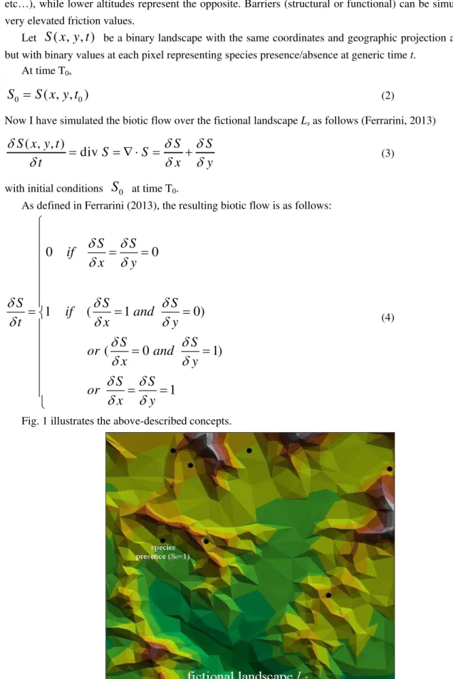
be a landscape where, for each pixel, the z-value is equal to the friction for the species under study. In other words, Ls is a 3D fictional landscape with the same coordinates and geographic

etc…), while lower altitudes represent the opposite. Barriers (structural or functional) can be simulated using

very elevated friction values.

Let

S x y t

( , , )

be a binary landscape with the same coordinates and geographic projection as Ls and L,

but with binary values at each pixel representing species presence/absence at generic time t. At time T0,

0

( , , )

0

S



S x y t

(2)

Now I have simulated the biotic flow over the fictional landscape Ls as follows (Ferrarini, 2013)

( , , )

div

S x y t

S

S

S

S

t

x

y











   







(3)

with initial conditions

S

₀ at time T0.

As defined in Ferrarini (2013), the resulting biotic flow is as follows:

0

0

1 (

1

0)

(

0

1)

1

S

S

if

x

y

S

S

S

if

and

t

x

y

S

S

or

and

x

y

S

S

or

x

y

























































_



























(4)

Fig. 1 illustrates the above-described concepts.

My model assumes that the species dispersal ends at a stability point, if exists, where:

( , , )

0

S x y t

S

t





   

(5)

Now, I define P as the predicted path for the species over the fictional landscape Ls, and P* the real path

followed by the species as detected by GPS data-loggers or in situ observations. The prediction bias B between

P and P* can hence be calculated as (Fig. 2)

*

mod(

)

B





Pdx





P dx

(6)

where the function mod indicates the module of the difference, hence:

* *

* *

where >

where

>

Pdx

P dx

P P

B

P dx

Pdx

P

P



_



 













(7)

Now, reverse flow connectivity acts as follows:

set B to 0 (8)

or, at least,

minimize B (9)

by optimizing



( )

L

under the constraints that

( )

0

( )

, with integer value

i

i

L

i

L

n

i

n













_

_



(10)

In other words, reverse flow connectivity assigns realistic resistance values to each land cover type by making

null the bias B between the predicted dispersal and the detected one. To do this, it builds up the fictional 3D

landscape

L x y

_s

( , , ( ))



L

so that the predicted biotic flow P corresponds to the one (i.e. P*) detected in situ.

The optimization of



( )

L

can be properly achieved using genetic algorithms (GAs; Holland, 1975). In

order to apply reverse flow connectivity modelling to real landscapes, I wrote the ad hoc software Reverse

Connectivity Lab (Ferrarini, 2013b). GAs are powerful evolutionary models with wide potential applications

in ecology and biology, such as optimization of protected areas (Parolo et al., 2009), optimal sampling

(Ferrarini, 2012c; Ferrarini, 2012d) and networks control (Ferrarini, 2011b; Ferrarini, 2013c; Ferrarini, 2013d;

Ferrarini, 2013e).

There are two useful suggestions when seeking true-to-life values for landscape resistance values. First, it

is always better to start with a 3D fictional landscape

L x y

_s

( , , ( ))



L

built upon friction values taken from

literature. In this way, it’s likely that reverse flow connectivity might need just minor corrections to such

values when optimizing



( )

L

in order to set B to 0. Instead, if the researcher starts from completely

unknown values for



( )

L

(e.g. friction values set to 0 for each land category), it is possible that the

computational effort becomes very high for common computers. Of course, the computational effort also

depends on the number of land categories and on the length of the path P*. Secondly, a potential drawback

arises when the real path P* does not meet all the land cover categories present in the landscape. In this case,

reverse flow modelling will be only able to assign resistance values to those land categories that have been

intersected by P*.

3 Conclusions

The pivotal topic in connectivity ecology is how to assign realistic resistance (frictional) values to landscape

categories. Based on these values and on the dispersal model, a large number of ecological processes can be understood, and many environmental management goals can be achieved such as preserving plant and animal populations, predicting infective disease spread and conserving biodiversity.

While in a previous paper (Ferrarini, 2013) I proposed a connectivity model and conceptual framework that is alternative to circuit theory, in this paper I have proposed an advance to flow connectivity that is able to

assign true-to-life frictional values to landscape categories. Thanks to the conceptual and operative framework proposed here, named reverse flow connectivity, the subjectivity in ecological connectivity is minimized and proper prediction of population dispersals across landscape is now possible.

Since connectivity is a pillar of metapopulation theory and gene flow, reverse flow connectivity can be regarded as a contribution to different fields such as ecology, biology and landscape genetics. Reverse flow

References

Cohen D, Levin SA. 1991. Dispersal in patchy environments: the effects of temporal and spatial structure.

Theoretical Population Biology, 39: 63-99

Crooks KR, Sanjayan M. 2006. Connectivity Conservation. Cambridge University Press, UK

Ferrarini A. 2005. Analisi e valutazioni spazio-temporale mediante GIS e Telerilevamento del grado di

Pressione Antropica attuale e potenziale gravante sul mosaico degli habitat di alcune aree italiane. Ipotesi di pianificazione. Ph.D. Thesis, Università degli Studi di Parma, Parma, Italy

Ferrarini A, Bollini A, Sammut E. 2010. Digital Strategies and Solutions for the Remote Rural Areas Development. Acts of Annual MeCCSA Conference, London School of Economics, London, UK

Ferrarini A, Tomaselli M. 2010. A new approach to the analysis of adjacencies. Potentials for landscape

insights. Ecological Modelling, 221: 1889-1896

Ferrarini A. 2011. Network graphs unveil landscape structure and change. Network Biology, 1(2): 121-126

Ferrarini A. 2011b. Some thoughts on the controllability of network systems. Network Biology, 1(3-4): 186-188

Ferrarini A. 2012. Founding RGB Ecology: the ecology of synthesis. Proceedings of the International

Academy of Ecology and Environmental Sciences, 2(2): 84-89

Ferrarini A. 2012b. Landscape structural modeling. A multivariate cartographic exegesis. In: Ecological

Modeling (Zhang WJ, ed). 325-334, Nova Science Publishers Inc., New York, USA

Ferrarini A. 2012c. Biodiversity optimal sampling: an algorithmic solution. Proceedings of the International Academy of Ecology and Environmental Sciences, 2(1): 50-52

Ferrarini A. 2012d. Betterments to biodiversity optimal sampling.Proceedings of the International Academy of Ecology and Environmental Sciences, 2(4): 246-250

Ferrarini A. 2013. A criticism of connectivity in ecology and an alternative modelling approach: Flow connectivity. Environmental Skeptics and Critics, 2(4): 118-125

Ferrarini A. 2013b. Reverse Connectivity Lab. Manual (in Italian)

Ferrarini A. 2013c. Controlling ecological and biological networks via evolutionary modelling. Network Biology, 3(3): 97-105

Ferrarini A. 2013d. Computing the uncertainty associated with the control of ecological and biological systems. Computational Ecology and Software, 3(3): 74-80

Ferrarini A. 2013e. Exogenous control of biological and ecological systems through evolutionary modelling.

Proceedings of the International Academy of Ecology and Environmental Sciences, 3(3): 257-265

Gustafson EJ, Gardner R.H. 1996. The effect of landscape heterogeneity on the probability of patch

colonization. Ecology, 77: 94-107

Hanski I. 1994. A practical model of metapopulation dynamics. Journal of Animal Ecology, 63:151-162 Holland J.H. 1975. Adaptation in Natural And Artificial Systems: An Introductory Analysis with Applications

to Biology, Control and Artificial Intelligence. University of Michigan Press, Ann Arbor, USA

King AW, With KA. 2002. Dispersal success on spatially structured landscapes: when do spatial pattern and

dispersal behavior really matter? Ecological Modelling, 147: 23-39 McRae B.H. 2006. Isolation by resistance. Evolution, 60: 1551-1561

McRae BH, Beier P. 2007. Circuit theory predicts gene flow in plant and animal populations. Proceedings of

the National Academy of Sciences of the USA, 104:19885-19890

McRae BH, Dickson BG, Keitt TH, Shah VB. 2008. Using circuit theory to model connectivity in ecology and

conservation. Ecology, 10: 2712-2724

Ecology, 79: 2503-2515

Moilanen A, Nieminen M. 2002. Simple connectivity measures in spatial ecology. Ecology, 83: 1131-1145

Parolo G, Ferrarini A, Rossi G. 2009. Optimization of tourism impacts within protected areas by means of genetic algorithms. Ecological Modelling, 220: 1138-1147

Poethke HJ, Seitz A, Wissel C. 1996. Species survival and metapopulations: conservation implications from

ecological theory. In: Species Survival in Fragmented Landscapes (Settele J, Margules C, Poschlod P, Henle K, eds). Kluwer Academic Publishers, London, UK

Poethke A, Hovestadt T, Mitesser O. 2003. Local extinction and the evolution of dispersal rates: causes and correlations. American Naturalist, 161: 631-640

Taylor A.D. 1990. Metapopulations, dispersal, and predator–prey dynamics: an overview. Ecology, 71:

429-433

Wiegand T, Moloney KA, Naves J, Knauer F. 1999. Finding the missing link between landscape structure and

population dynamics: a spatially explicit perspective. American Naturalist, 154: 605-627

Wiens J.A. 2001. The landscape context of dispersal. In: Dispersal (Clobert J, Danchin E, Dhondt AA, Nichols JD, eds). Oxford University Press, UK