Article
Detecting barriers and facilities to species dispersal: Introducing
sloping flow connectivity
Alessandro Ferrarini
Department of Evolutionary and Functional Biology, University of Parma, Via G. Saragat 4, I-43100 Parma, Italy E-mail: [email protected], [email protected]
Received 28 April 2014; Accepted 2 June 2014; Published online 1 September 2014
Abstract
Connectivity in ecology deals with the problem of how biotic dispersals can happen, given actual landscape properties and species presence/absence over such landscape. Recently I have introduced a modelling approach (flow connectivity) to ecological connectivity that is alternative to circuit theory, and is able to fix the weak point of the “from-to” connectivity approach. In addition, I’ve introduced “reverse flow connectivity” that couples evolutionary algorithms to partial differential equations in order to fix the problem of subjectivity in the attribution of friction values to landscape categories. I’ve also showed that flow connectivity can be used to predict biotic movements happened in the past (backward flow connectivity). To date, there has been little effort by conservation scientists towards detecting restoration opportunities by mapping barriers that strongly reduce movement potential. In this paper, I introduce a new kind of theoretical and modelling approach called “sloping flow connectivity”. The goal of such proposal is to individuate and map barriers and facilities to species dispersals over the landscape. I define here a barrier as a landscape feature that impedes biotic movements, the removal of which would increase the potential for biotic shifts. Using sloping flow connectivity, it’s possible to plan greenways and ecological networks in an effective manner, since it is able to enhance the real potential of each landscape elements to facilitate or obstruct both directional and overall species movements.
Keywords biotic flows; dispersal facilities; flow connectivity; gene flow; landscape barriers; landscape connectivity; partial differential equations; species dispersal.
1 Introduction
1 Introduction
Predicting how animals disperse is a pivotal issue for the management and conservation of fragmented populations. Landscape heterogeneity and fragmentation affect how organisms are distributed in the landscape (Fahrig and Merriam, 1985; Kennedy and Gray, 1997), determine the chance of a patch being colonized (Hanski and Ovaskainen, 2000), reduce inbreeding in small populations and maintains evolutionary potential
Proceedings of the International Academy of Ecology and Environmental Sciences ISSN 22208860
URL: http://www.iaees.org/publications/journals/piaees/onlineversion.asp RSS: http://www.iaees.org/publications/journals/piaees/rss.xml
Email: [email protected] EditorinChief: WenJun Zhang
(Couvet, 2002). In order to predict dispersal, it is important to not only consider an organism’s dispersal capabilities, but also the complex interactions between its behaviour and the landscape pattern and use.
The modelling of animal dispersal provides a useful tool for investigating these complex interactions, and it is an essential goal for biotic conservation planning (Kareiva and Wennergren, 1995; King and With, 2002). Due to the difficulty in gathering experimental results on species dispersal, simulation models have become a cost-effective approach to predict dispersal dynamics (Tischendorf, 1997; Wiegand et al., 1999; Tischendorf and Fahrig, 2000). Simulation models with spatially-explicit landscapes enable the integration of the relationships between species and the landscape, and provide representation of the spatial elements that promote or constrain dispersal. Several dispersal models with spatially explicit landscapes have been developed. Some consider dispersal behaviour according to habitat affinity or physiological states in order to predict animal movements and provide guidelines for landscape and wildlife management (Gustafson and Gardner, 1996; With et al., 1997; Gardner and Gustafson, 2004).
Recently I have introduced a modelling approach (flow connectivity; Ferrarini, 2013a) to ecological connectivity that is alternative to circuit theory (McRae, 2006; McRae and Beier, 2007; McRae et al., 2008), and is able to fix the weak point of the “from-to” connectivity approach. Landscape connectivity as estimated by circuit theory relies on a strong assumption that is possibly untrue, unproven or very challenging to be demonstrated: species dispersals are “from-to” movements, i.e. from source points (patches) of the landscape to sink ones. Source and sinks are suitable areas present within a matrix that is partially or completely hostile to the species. There are two aspects of this approach that are questionable. First, a source-sink habitats model can be suitable to describe lowland landscapes where few suitable patches (e.g. protected areas) are surrounded by a dominant, hostile (or semi-hostile) anthropogenic landscape. By the way, can we think the same of mountain and hilly landscapes? Such landscapes are not composed of source and sink habitats, instead they’re a continuum with a natural matrix where the source-sink habitats model loses its rationale. Second, assuming that a species aims to go from “patch A” to “patch B” means that such species is supposed to plan such dispersal path (i.e. global optimization). This could be true for short-range dispersals where the final point is visible from the starting one, but for wide-range movements, and for plant species in particular, the dispersal model postulated by circuit theory is unsuitable.
In addition, I’ve introduced “reverse flow connectivity” (Ferrarini, 2014a) that couples evolutionary algorithms to partial differential equations in order to fix the problem of subjectivity in the attribution of friction values to landscape categories. I’ve also showed that flow connectivity can be used to predict biotic movements happened in the past (backward flow connectivity; Ferrarini, 2014b).
In this paper, I introduce a new kind of theoretical and modelling approach called “sloping flow connectivity”. The goal of such proposal is to individuate barriers (to be removed) and facilities (to be conserved) to species dispersal over the landscape. The reason behind sloping flow connectivity is that it makes possible to plan greenways and ecological networks in an effective manner, since it is able to enhance the real potential of each landscape elements to facilitate or obstruct directional and overall species movements.
2 Sloping Flow Connectivity: Mathematical Formulation
Let
L x y z t
( , , , )
be a real 3D landscape at generic time t, whereL[1,..., ]n . In other words, L is a generic (categorical) landcover or land-use map with n classes. At time T0,0
( , , , )
0L
L x y z t
(1)Let be the landscape friction (i.e. how much each land parcel is unfavourable) to the species under study. In other words,
( )
L
is a function that associates a friction value to each pixel of L. At time T0,0
(
L
0)
(2)Let
L x y
s( , , ( ))
L
be a landscape where, for each pixel, the z-value is equal to the friction for the speciesunder study. In other words, Ls is a 3D fictional landscape with the same coordinates and geographic
projection as L, but with pixel-by-pixel friction values in place of real z-values. Higher elevations represents areas with elevated friction to the species due to whatever reason (unsuitable landcover, human disturbance etc), while lower altitudes represent the opposite.
True-to-life coefficients for landscape friction can be calculated as in Ferrarini (2014a), where I defined P as the predicted path for the species over the fictional landscape Ls, and P* the real path followed by the
species as detected by GPS data-loggers or in situ observations. The bias B between P and P* is hence calculated as
*
mod(
)
B
Pdx
P dx
(3)where the function mod indicates the module of the difference. Hence:
* *
* *
where >
where
>
Pdx
P dx
P P
B
P dx
Pdx
P P
(4)Now, true-to-life coefficients for landscape friction can be calculated by optimizing B, as follows:
set B to 0 (5)
or, at least,
minimize B (6)
The optimization of
( )
L
can be properly achieved using genetic algorithms (GAs; Holland, 1975). GAs are powerful evolutionary models with wide potential applications in ecology and biology, such as optimization of protected areas (Ferrarini et al.,2008; Parolo et al., 2009), optimal sampling (Ferrarini, 2012a; Ferrarini, 2012b), optimal detection of landscape units (Rossi et al., 2014) and networks control (Ferrarini, 2011a; Ferrarini, 2013b; Ferrarini, 2013c; Ferrarini, 2013d; Ferrarini, 2013e; Ferrarini, 2014c). At time T0,(7)
Now, sloping flow connectivity acts upon the optimized frictional landscape of eq. (7) as follows:
0
( , , (
))
( , )
s
L x y
L
v x y
(8)In other words, sloping flow connectivity calculates (pixel-by-pixel) the slope of the optimized frictional landscape along the (vectorial) direction v that is a function of x and y dimensions:
v
ax b y
(9)For instance, with a= 0 and b= 1 eq (8) calculates the frictional slope toward the N direction; with a = 1 and b= 1, eq. (8) calculates the frictional slope toward the N-E direction. Since a and b are real numbers, sloping connectivity is able to calculate slope not only along the 8 cardinal directions (N, E, S, O, N-E, S-E, N-O, S-O), but along any compass bearing.
In order to estimate the slope of a landscape cell along a particular direction, sloping flow connectivity acts as follows:
0
( , , (
0))
s s
0
( , , ( ))
( , )
s v
h
L x y
L
D
D
v x y
(10)where Dv and Dh are the vertical and horizontal distances between the center-point of the focal cell and the
center-point of the adjacent cell in the specified direction.
Sloping flow connectivity takes a reasonably simple approach to estimate the % slope of a cell in a particular direction: it assumes that the elevation values for all cells are good estimates of the elevation at the center-points of the cells. If the direction is not a cardinal direction, then the slope is calculate from the focal cell center-point to an interpolated point between 2 adjacent cell center-points. It can also be calculated in degrees using the following alternative equation:
0
( , , (
))
180
arctan(
) *
( , )
s v
h
L x y
L
D
D
v x y
(11)Which is the ecological meaning of the slope direction (also known as, slope aspect or slope orientation) calculated over the frictional landscape Ls? Clearly, it represents the least friction direction (LFD) to species
dispersal. To calculate the aspect from the frictional landscape Ls, I have used the equation from Evans (1972):
0 0
( , , (
))
arctan
( , , (
))
s sL x y
L
y
LFD
L x y
L
x
(12)which is the angle by the x and y derivative of Ls via arctan, measured clockwise in degrees from North. Once
LFD is calculated, it can be then grouped into 9 categories (flat; N: 337.58–22.58, NE: 22.58–67.58, E: 67.58–112.58, SE: 112.58–157.58, S: 157.58–202.58, SW: 202.58–247.58, W: 247.58–292.58, NW: 292.58–337.58).
In order to apply sloping flow connectivity modelling to real landscapes, I wrote the ad hoc software Connectivity Lab (Ferrarini, 2013f).
3 An Applicative Example
The Ceno valley is a 35,038 ha wide valley situated in the Province of Parma, Northern Italy. It has been mapped at 1:25,000 scale (Ferrarini, 2005; Ferrarini et al., 2010) using the CORINE Biotopes classification system. The landscape structure of the Ceno Valley has been widely analysed (Ferrarini and Tomaselli, 2010; Ferrarini, 2011b; Ferrarini, 2012c; Ferrarini, 2012d).
From an ecological viewpoint, the most interesting event registered in the last years is the shift of wolf populations from the montane belt to the lowland. Several populations have been recently observed insitu by life-watchers, environmental associations and local administrations.
As an example of sloping flow connectivity, I have applied my model to a portion of the Ceno valley (Fig. 1) above 1000 m a.s.l. close to the municipality of Bardi where several small populations of wolveshave been
recently observed. The area is a square of about 20 km * 20 km. Optimized friction values to wolf
presence are borrowed from Ferrarini (2012e) in the form of friction coefficients assigned to every land cover classes. A discussion of wolf’s frictional coefficients is outside the goals of this paper, so I avoid presenting them.
Fig. 1 The frictional landscape Ls has been built for wolf upon a 20 km * 20 km portion of the Ceno Valley (province of Parma, Italy) that represents here the real landscape L(x,y,z,t). The higher frictional values are in red, the lower ones are in blue. The frictional landscape has been built using both structural and functional properties of the landscape (Ferrarini, 2012e).
In order to simulate (directional) species movements along such landscape, I calculated sloping flow connectivity along the 4 cardinal directions (N, S, E, O) using equations from (8) to (12).
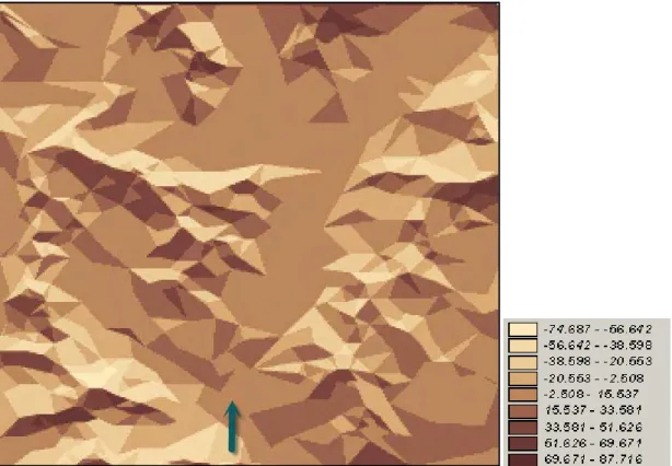
Simulated northward (i.e., a= 0 and b= 1) connectivity is depicted in Fig. 2. Darker areas depict the individuated barriers, lighter ones are the detected facilities. Barriers to northward wolf’s movements are present in particular in the Eastern and Western portions of the study area. Instead, the central part of the study area present less problems to northward wolf’s movements.
Fig. 2 Simulated wolf’s northward movements (as indicated by the arrow). Darker areas represent the individuated barriers, lighter ones are the detected facilities.
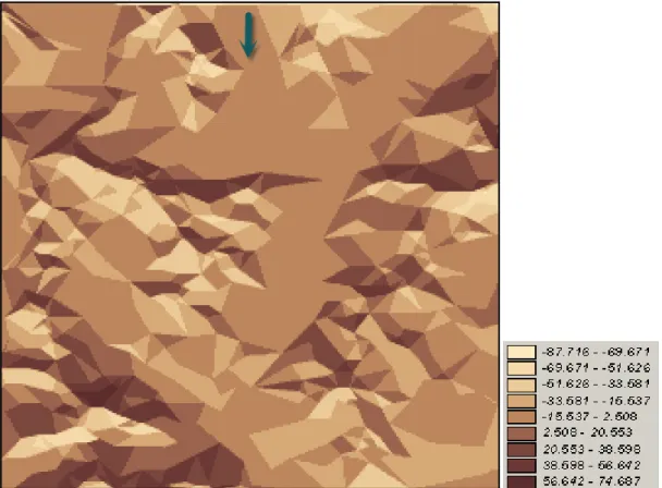
Fig. 4 Simulated wolf’s southward movements (as indicated by the arrow). Darker areas represent the individuated barriers, lighter ones are the detected facilities.
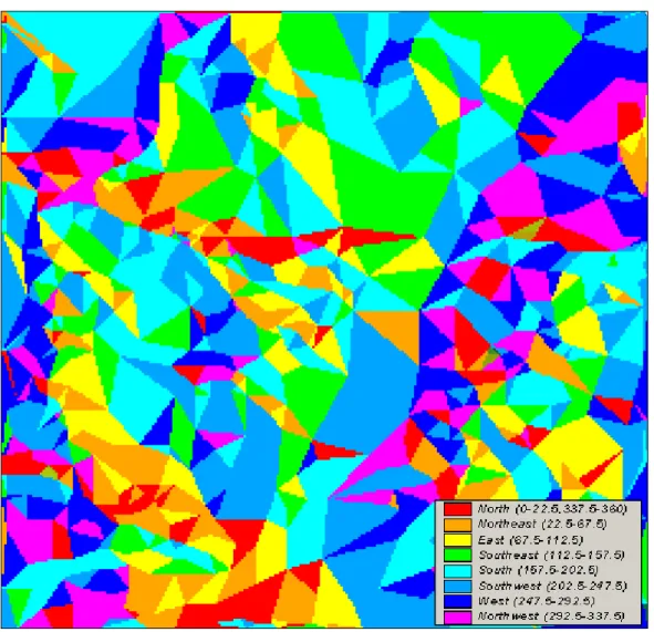
The computation of the LFD for the frictional landscape Ls using eq. (12)depicts for each portion of the study area the most facilitated direction for wolf (Fig. 6).
It results clear that wolf’s movements towards South, South-West and West are the most probable (i.e. facilitated) events in the study area. Instead, wolf’s movements towards North, North-East and East are highly improbable. It’s also clear that there’s a kind of spatial clustering of movements probabilities, with certain directions prevalent in particular portions of the study area (Fig. 6).
Fig. 6 Map of the most facilitated wolf’s movements in the study area. It has been achieved via sloping flow connectivity applied to the frictional landscape Ls of Fig. 1. For each pixel, the direction with the lowest friction to species dispersal is given.
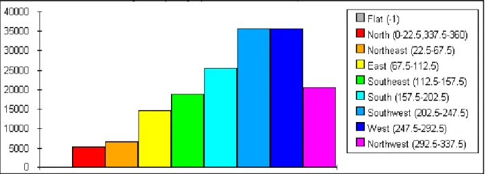
Fig. 7 Histogram of the most facilitated directions to wolf’s dispersal in the study area. Columns count the number of pixels in the sloping landscape of Fig. 6 with a particular direction for the most facilitated wolf’s dispersal.
4 Conclusions
Planning greenways and ecological networks in an effective manner is not an easy task, since it requires to detect the real potential of each landscape elements to facilitate or obstruct both directional and overall species movements. Conservation practitioners use two main strategies to promote connectivity. The first focalizes on conserving areas that facilitate movement, the second focuses on restoring connectivity across areas that impede movement. Most connectivity works have focused on the former strategy.
In this paper, I have introduced sloping flow connectivity that is on top of this requirement, as it is able to produce simple and effective maps of barriers and facilities to directional and overall species dispersal. Sloping flow connectivity takes advantage of two previously-introduced theoretical and methodological frameworks for the prediction of species dispersal: flow connectivity and reverse flow connectivity.
References
Couvet D. 2002. Deleterious effects of restricted gene flow in fragmented populations. Conservation Biology, 16: 369-376
Evans I.S. 1972. General geomorphometry, derivations of altitude and descriptive statistics. In: Chorley R.J. (Editor). Spatial analysis in geomorphology. 17-90, Harper & Row Publishers, New York, USA
Fahrig L, Merriam G. 1985. Habitat patch connectivity and population survival. Ecology, 66: 1762-1768 Ferrarini A. 2005. Analisi e valutazioni spazio-temporale mediante GIS e Telerilevamento del grado di
Pressione Antropica attuale e potenziale gravante sul mosaico degli habitat di alcune aree italiane. Ipotesi di pianificazione. Ph.D. Thesis, Università degli Studi di Parma, Parma, Italy
Ferrarini A, Rossi G, Parolo G, Ferloni M. 2008. Planning low-impact tourist paths within a Site of
Community Importance through the optimisation of biological and logistic criteria. Biological Conservation, 141:1067-1077
Ferrarini A, Tomaselli M. 2010. A new approach to the analysis of adjacencies. Potentials for landscape insights. Ecological Modelling, 221:1889-1896
Ferrarini A. 2011a. Some thoughts on the controllability of network systems. Network Biology, 1(3-4): 186-188
Ferrarini A. 2011b. Network graphs unveil landscape structure and change. Network Biology, 1(2): 121-126 Ferrarini A. 2012a. Biodiversity optimal sampling: an algorithmic solution. Proceedings of the International
Academy of Ecology and Environmental Sciences, 2(1): 50-52
Ferrarini A. 2012b. Betterments to biodiversity optimal sampling.Proceedings of the International Academy of Ecology and Environmental Sciences, 2(4): 246-250
Ferrarini A. 2012c. Founding RGB Ecology: the Ecology of Synthesis. Proceedings of the International Academy of Ecology and Environmental Sciences, 2(2): 84-89
Ferrarini A. 2012d. Landscape structural modeling. A multivariate cartographic exegesis. In: Ecological Modeling (Zhang WJ, ed). 325-334, Nova Science Publishers Inc., New York , USA
Ferrarini A. 2012e. The ecological network of the province of Parma. Province of Parma, Parma, Italy (in Italian)
Ferrarini A. 2013a. A criticism of connectivity in ecology and an alternative modelling approach: Flow connectivity. Environmental Skeptics and Critics, 2(4): 118-125
Ferrarini A. 2013b. Controlling ecological and biological networks via evolutionary modelling. Network Biology, 3(3): 97-105
Ferrarini A. 2013c. Computing the uncertainty associated with the control of ecological and biological systems. Computational Ecology and Software, 3(3): 74-80
Ferrarini A. 2013d. Exogenous control of biological and ecological systems through evolutionary modelling.
Proceedings of the International Academy of Ecology and Environmental Sciences, 3(3): 257-265
Ferrarini A. 2013e. Networks control: Introducing the degree of success and feasibility. Network Biology, 3(4): 127-132
Ferrarini A. 2013f. Connectivity-Lab 2.0: a software for applying connectivity-flow modelling. Manual, Italy (in Italian)
Ferrarini A. 2014a. True-to-life friction values in connectivity ecology: Introducing reverse flow connectivity. Environmental Skeptics and Critics, 3(1): 17-23
Ferrarini A. 2014b. Can we trace biotic dispersals back in time? Introducing backward flow connectivity. Environmental Skeptics and Critics, 3(2): 39-46
Ferrarini A. 2014c. Local and global control of ecological and biological networks. Network Biology, 4(1): 21-30
Gardner RH, Gustafson E.J. 2004. Simulating dispersal of reintroduced species within heterogeneous landscapes. Ecological Modelling, 171: 339-358
Gustafson EJ, Gardner R.H. 1996. The effect of landscape heterogeneity on the probability of patch colonization. Ecology 77, 94–107
Hanski I, Ovaskainen O. 2000. The metapopulation capacity of a fragmented landscape. Nature, 404: 755-758 Holland J.H. 1975. Adaptation in Natural And Artificial Systems: An Introductory Analysis with Applications
to Biology, Control and Artificial Intelligence. University of Michigan Press, Ann Arbor, USA
Kareiva P, Wennergren U. 1995. Connecting landscape patterns to ecosystem and population processes. Nature, 373: 299-302
King AW, With KA. 2002. Dispersal success on spatially structured landscapes: when do dispersal pattern and dispersal behaviour really matter? Ecological Modelling 147: 23-39
McRae BH. 2006. Isolation by resistance. Evolution, 60: 1551-1561
McRae BH, Beier P. 2007. Circuit theory predicts gene flow in plant and animal populations. Proceedings of the National Academy of Sciences of the USA, 104: 19885-19890
McRae BH, Dickson BG, Keitt TH, Shah VB. 2008. Using circuit theory to model connectivity in ecology and conservation. Ecology, 10: 2712-2724
Parolo G, Ferrarini A, Rossi G. 2009. Optimization of tourism impacts within protected areas by means of genetic algorithms. Ecological Modelling, 220: 1138-1147
Rossi G, Ferrarini A, Dowgiallo G, Carton A. et al. 2014. Detecting complex relations among vegetation, soil and geomorphology. An in-depth method applied to a case study in the Apennines (Italy). Ecological Complexity, 17(1): 87-98
Tischendorf L. 1997. Modelling individual movements in heterogeneous landscapes: potentials of a new approach. Ecological Modelling 103: 33-42
Tischendorf L, Fahrig L. 2000. How should we measure landscape connectivity? Landscape Ecology 15, 633– 641
Wiegand T, Moloney K, Naves J, Knauer F. 1999. Finding the missing link between landscape structure and population dynamics: a spatially explicit perspective. American Naturalist, 154: 605-627
With KA, Gardner RH, Turner M.G. 1997. Landscape connectivity and population distributions in heterogeneous environments. Oikos, 78: 151-169